A Two-Stage Distributionally Robust Optimization Model for Managing Electricity Consumption of Energy-Intensive Enterprises Considering Multiple Uncertainties

Abstract

Energy-intensive enterprises (EIEs), as vital demand-side flexibility resources, can significantly enhance the power system’s ability to regulate demand by participating in demand response (DR). This helps alleviate supply pressures during tight demand–supply conditions, ensuring the system’s safe and stable operation. However, due to the current level of electricity management in EIEs, their participation in demand response has disrupted the continuity of production to some extent, which may hinder the sustainability of demand-side management mechanisms. To address this issue, this paper proposes a two-stage distributionally robust optimization (DRO) model for managing production electricity in EIEs, considering multiple uncertainties. First, a production electricity load model based on the state task network (STN) is developed, reflecting the characteristics of industrial production lines. Next, a two-stage DRO model for day-ahead and intra-day electricity management is formulated, integrating an uncertainty set for distributed generation output based on the Wasserstein distance and probabilistic constraints for the day-ahead DR capacity. Finally, a cement plant in western China is used as a case study to validate the effectiveness of the proposed model. The results show that the proposed model effectively guides EIE in participating in DR while optimizing electricity costs, enabling cost savings of up to 27.7%.

1. Introduction

As power systems move toward decarbonization, the integration of variable renewable energy (VRE), primarily wind and solar, is increasingly prevalent in power grids. However, the intermittent nature of VRE presents significant challenges to grid stability and reliability [1]. Recently, there has been a growing interest in improving system flexibility to address these fluctuations, with demand-side flexibility emerging as a promising solution. Energy-intensive enterprises (EIEs) can play a critical role in strengthening grid flexibility due to their substantial regulatory capacity, rapid response capabilities, and high operational stability [2]. Despite this potential, existing methods to improve the flexibility of grids through EIE suffer from several major drawbacks: insufficient refinement, weak integration with production processes, and limited consideration of user interests [3].

Previous studies have primarily reported on EIEs from the perspective of the grid, focusing on scheduling strategies and evaluating the effectiveness of demand response. For example, reference [4] proposes a set of joint scheduling models for EIEs in power system dispatch, analyzing their benefits in supporting large-scale VRE integration. Similarly, reference [5] uses multi-objective optimization to model constraints related to switching capacity and frequency for EIEs, such as electrolytic aluminum and iron alloys, developing scheduling plans for both generators and EIEs. These studies have contributed significantly to the advancement of VRE integration. However, several challenges still need to be solved with grid-centered scheduling models for EIEs. First, these models are often overly simplified, failing to account for the impact of regulation on production processes, making it challenging to accurately reflect internal adjustments. Secondly, evaluating the benefits of EIEs participating in demand-side management (DSM) is inadequate, as these models overlook the effects of grid scheduling on production objectives, thereby limiting the sustainable development of DSM mechanisms. Lastly, these limitations result in discrepancies between actual response outcomes and model predictions, posing potential risks to grid operators’ decision-making processes.

Few published studies have attempted to refine energy management strategies for EIEs compared to grid-centered models. However, such refinements provide the dual benefits of reducing energy costs for EIEs and alleviating pressure on the power grid. Reference [6] presents a scheduling model that improves industrial energy efficiency by integrating distributed generation and demand response while also considering the continuity of the product inventory. However, this model does not fully account for phased production tasks or the dynamic characteristics of product states throughout the production process. Reference [7] uses an approach using an artificial neural network to establish an optimized scheduling model for steel powder production plants but does not take into account phased production tasks and production objectives. In general, most of these studies have not taken into account the complex nature of industrial production processes and the dynamic interaction between energy supply and production tasks, reducing the practical applicability of the model. More work is needed to develop models that are tailored to EIEs.

To achieve a more precise modeling of electricity consumption characteristics in EIEs, several studies have introduced the state task network (STN) [8] and resource task network (RTN) [9] frameworks. For example, reference [10] investigates a battery manufacturing plant with highly sequential production processes, developing an integrated energy scheduling model within the RTN framework to optimize operational efficiency while considering various production constraints. Similarly, reference [11] formulates a mathematical model for managing the electricity consumption of production equipment using the STN and proposes an intelligent electricity management strategy for industrial users. These studies provide detailed mathematical descriptions of electricity consumption patterns and the impact of regulatory actions on production processes. However, they often focus on isolated factors, such as the complexity of industrial production, or limit their analysis to basic price-based demand response scenarios, like time-of-use pricing. What remains unclear is how electricity consumption strategies can be adapted to respond to more complex demand response signals from the grid, especially in managing the uncertainties associated with these signals.

Without loss of generality, EIEs often occupy large areas and commonly install distributed generation (DG) systems on site to reduce overall energy costs [12]. However, previous research has largely overlooked the impact of uncertainty in DG’s output on electricity management practices for these companies. This uncertainty presents a significant risk that should not be ignored. Distributionally robust optimization (DRO) [13], an emerging approach to uncertainty modeling, addresses the challenges of obtaining accurate probability distribution parameters in stochastic optimization while reducing the conservatism typical of traditional robust optimization. By combining the strengths of both approaches, DRO has been successfully applied in various energy systems and microgrids [14,15]. To address the effects of DG output uncertainty on electricity management for production, this study explores DRO-based scheduling strategies tailored to EIEs. It provides new insights into how EIEs can optimize electricity consumption in complex environments with uncertainties in DG output and DR signals.

In summary, previous research on EIE participation in DR strategies has the following shortcomings:

• Most existing studies adopt a power grid-centric perspective when modeling the DR capabilities of energy-intensive enterprises (EIEs), relying primarily on macroscopic estimations of their response capacity during DR periods. These approaches often overlook the continuity constraints inherent in production processes, resulting in response strategies that lack integration with the actual operational workflows of the enterprises. Consequently, from the grid perspective, the authenticity of the DR capabilities of EIEs remains uncertain. Moreover, for EIE users, such methods do not maximize the economic benefits of their participation in DR programs.
• Many studies employ deterministic models. From an internal perspective, they often overlook the impact of uncertainties in the DG output on response strategies. From an external perspective, they may not consider the uncertainties associated with the DR signals issued by the power grid, further reducing the robustness and applicability of the proposed strategies. When such uncertainties occur under adverse scenarios, they can significantly undermine the economic efficiency of energy management for EIE users.

To address the aforementioned issues, the primary contributions of this paper are as follows.

• The electricity consumption characteristics of EIEs are modeled in detail using the state task network (STN), specifically tailored to the features of process industries.
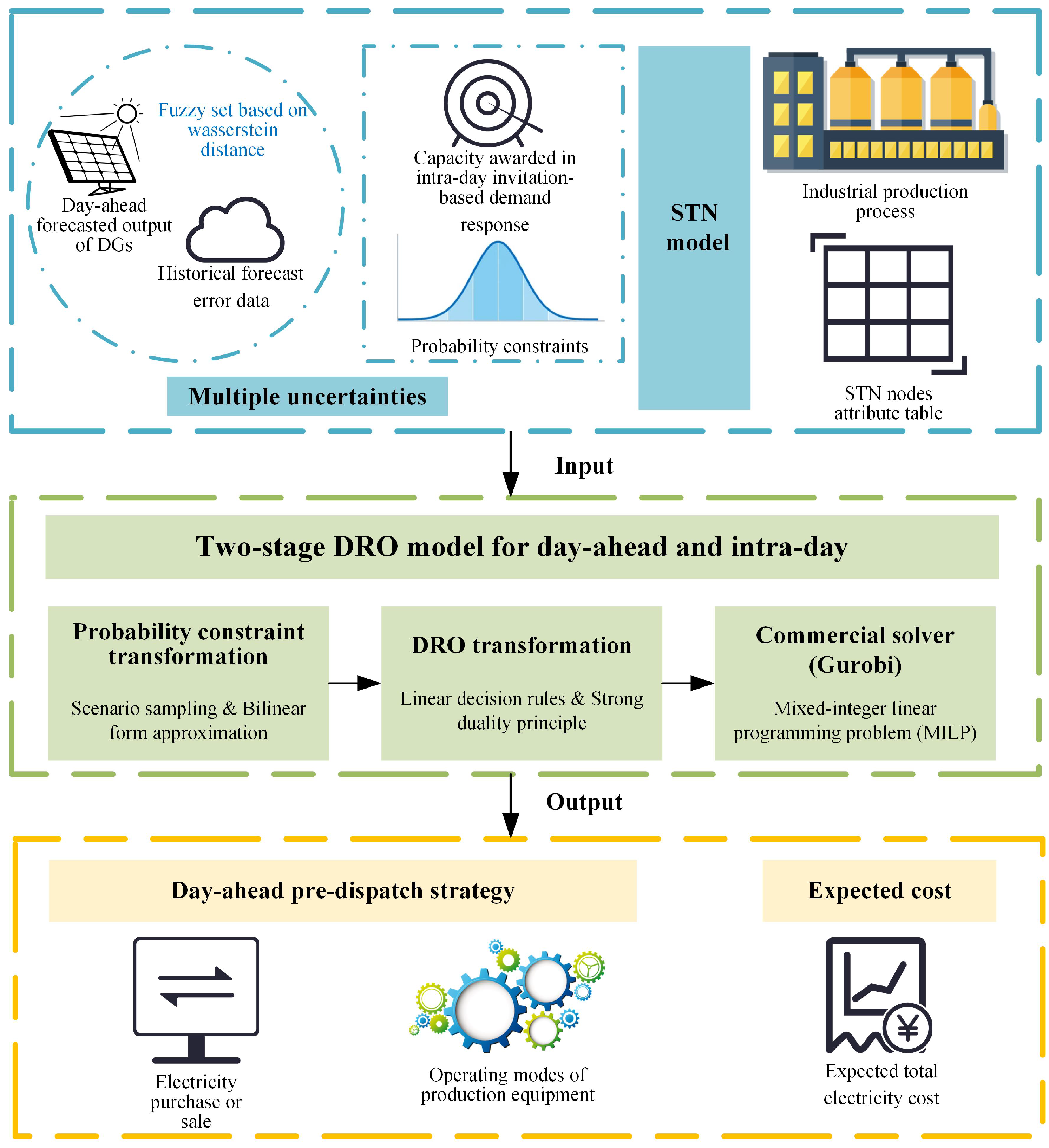
• A two-stage distributionally robust optimization (DRO) model is developed to address the uncertainty risks associated with DG output in EIEs. It incorporates both day-ahead pre-scheduling and intra-day rescheduling. Through rigorous mathematical transformations, the model is converted into an MILP problem, allowing it to be solved using commercial solvers (such as Gurobi), thereby improving its computational efficiency.
• The model considers the complex demand response signals from the grid, explicitly addressing the uncertainty in the awarded capacity during the intra-day period. Additionally, by simplifying the model, it is possible to calculate the DR potential of EIEs while considering their economic interests, providing valuable insights for the grid in implementing DR strategies.

2. Methodology

2.1. Overview

Figure 1 shows the optimizing electricity strategies for EIEs. Users interact with the electricity market through a dual payment mechanism [16], encompassing both day-ahead and intra-day transactions, and also participate in invitation-based demand response programs during the intra-day period. To improve the dispatching efficiency of industrial production tasks while meeting operational needs, electricity consumption management is structured into two stages: day-ahead pre-dispatch and intra-day re-dispatch.

To begin this process, the day-ahead output of DGs is forecasted using historical data analysis and numerical weather prediction models [17]. Before incorporating the forecasted data, an uncertainty set for DG output is developed based on the Wasserstein metric [18], and DR uncertainty is represented through probabilistic constraints. After these elements are defined, they are integrated into the STN model and a two-stage DRO algorithm to facilitate day-ahead and intra-day scheduling. Following a series of transformations, including an affine adjustment strategy, probability constraint transformation, and dual transformation, the model is structured for compatibility with commercial solvers (such as Gurobi), thereby enhancing its computational efficiency. Finally, the model’s optimized scheduling can be executed based on the defined constraints and uncertainties.

The resulting day-ahead pre-dispatch strategy balances scheduling economics with risk robustness. Additionally, the total expected electricity costs for both the day-ahead and intra-day stages are calculated. This strategy includes detailed plans for electricity purchases and sales, as well as operational strategies for production equipment.

Due to space constraints, this paper includes a case study focused on a cement plant in western China, as cement plants represent a common and significant category of EIE in the region. It should be noted that the proposed methodology is also applicable to other types of EIEs, such as those in the iron and steel industry and the electrolytic aluminum sector.

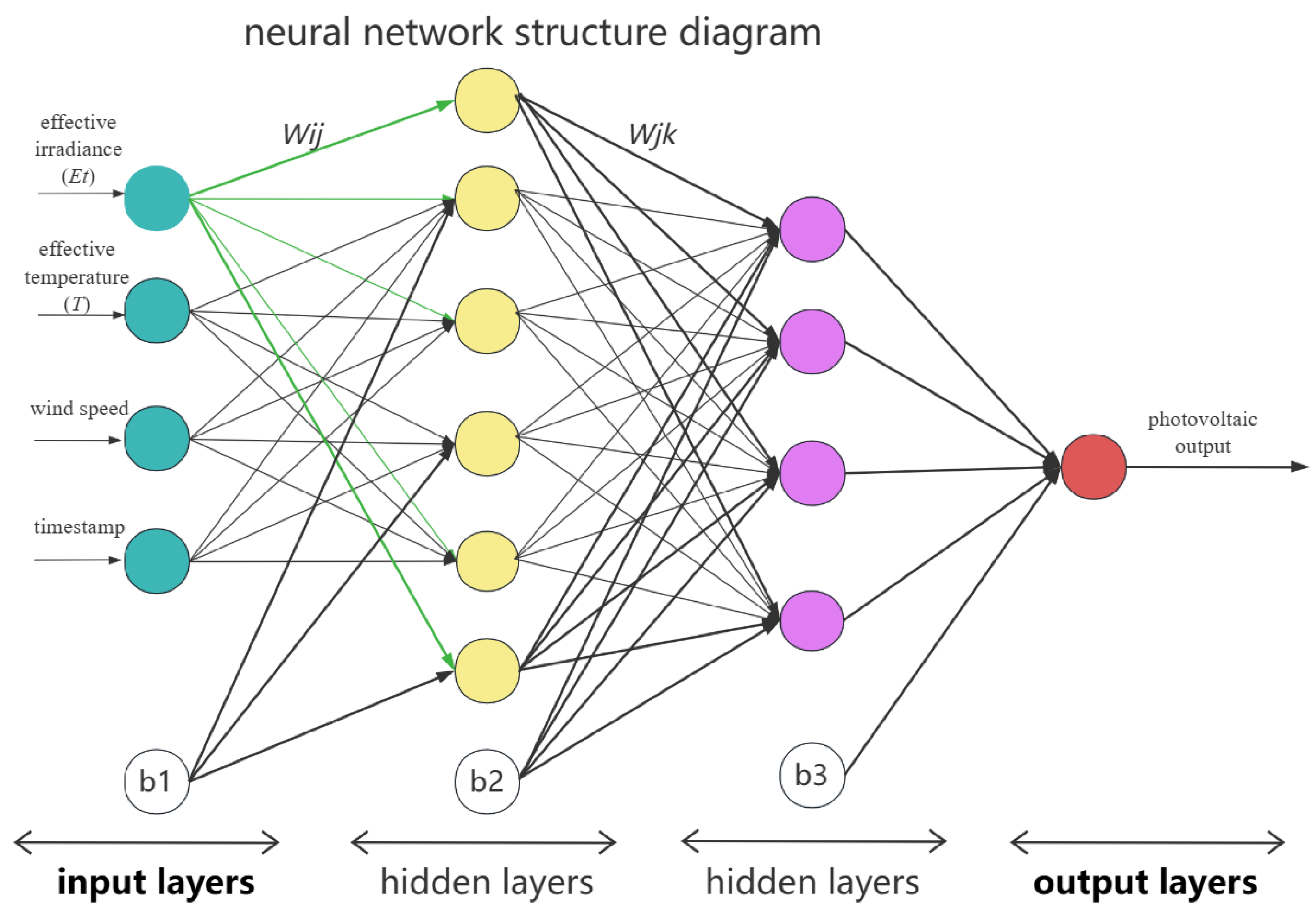
2.2. DG Output Prediction Model

The steps for DG output prediction based on numerical weather prediction are as follows:

• Obtain historical meteorological data, including irradiance, temperature, and wind speed, for the location of the photovoltaic power plant, along with the corresponding power output of the photovoltaic plant for each record.
• Data processing: specifically, the irradiance is adjusted to the effective irradiance of the photovoltaic panels, and the temperature is corrected to the effective temperature of the photovoltaic panels, thereby generating the modified meteorological data, which are corrected using the following formulas:

  $$\begin{array}{cc}\hfill E_t& =E_{b}cos\left(\mathrm{Inc}\right)+E_d\left({\displaystyle \frac{1+cos\left(\mathrm{Tilt}\right)}{2}}\right)+\mathrm{Ref}{E}_h\left({\displaystyle \frac{1-cos\left(\mathrm{Tilt}\right)}{2}}\right)\hfill \end{array}$$

  (1)

  $$\begin{array}{cc}\hfill \mathrm{T}& ={\mathrm{T}}_{\mathrm{air}}+\mathrm{K}\mathrm{S}\hfill \end{array}$$

  (2)
  In the equations, $E_t$ represents the effective irradiance of the photovoltaic panel, $E_b$ is the direct irradiance, $E_d$ is the diffuse irradiance, and $E_h$ is the total irradiance on the horizontal plane. $\mathrm{Tilt}$ is the tilt angle of the photovoltaic panel, $\mathrm{Inc}$ is the solar incidence angle, and $\mathrm{Ref}$ is the reflectivity coefficient. $\mathrm{T}$ is the effective temperature of the photovoltaic panel, ${\mathrm{T}}_{\mathrm{air}}$ is the ambient temperature, $\mathrm{S}$ is the solar irradiance, and $\mathrm{K}$ is the temperature coefficient.
• Training: the corrected meteorological data is used as input to the neural network, with the corresponding photovoltaic power generation output for each set of meteorological data serving as the output. The neural network is then trained using these input–output pairs.
• Output: the corrected meteorological data are input into the trained neural network, and the network outputs the power generation of the photovoltaic power plant for the corresponding prediction period.

The network architecture diagram for photovoltaic output prediction is shown in Figure 2.

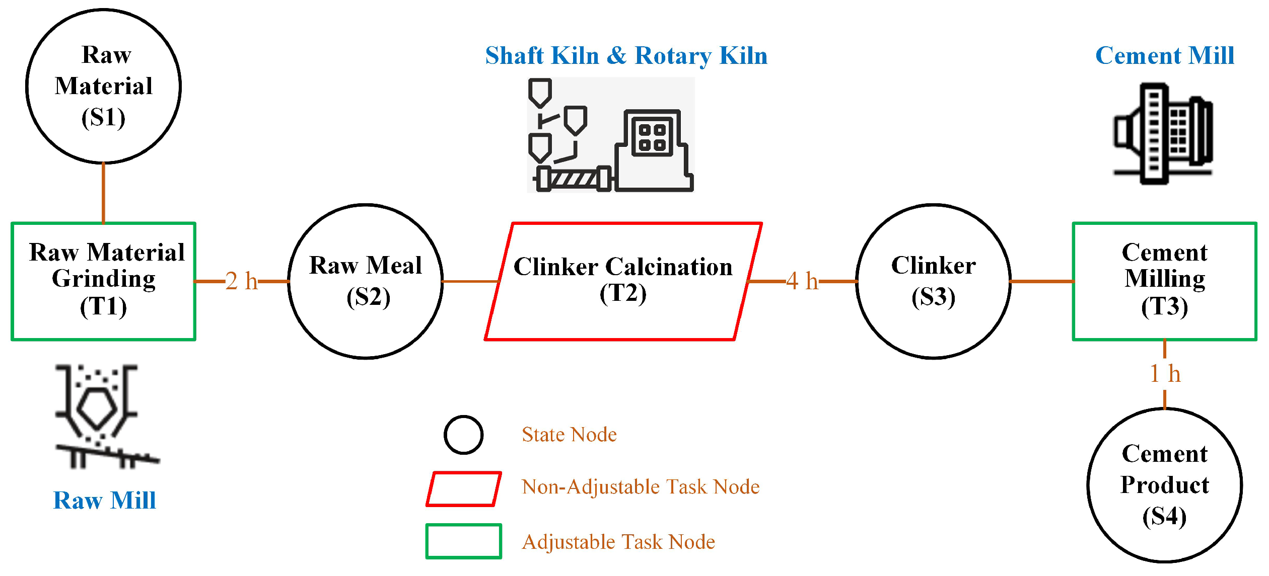
2.3. Production Process Modeling—State Task Network

To enhance the model’s general applicability, this paper adopts the STN framework to develop an optimized scheduling model tailored for industrial production tasks. This approach optimizes production processes in process industries, where most EIEs are classified. Within the STN framework, two types of nodes are defined: state nodes and task nodes. State nodes represent material inventories at various stages of production, including raw materials, intermediates, and final products. Critical parameters for state nodes include storage limits, production targets, and other relevant attributes. Task nodes, on the other hand, represent production activities, with parameters detailing the electrical power requirements and equipment production rates involved in each task.

In the STN framework, task nodes are further categorized as either adjustable or non-adjustable, based on whether the production rate can be modified. Non-adjustable tasks have fixed production rates throughout each period of the scheduling cycle, meaning the power load of the associated equipment remains constant, leading to a stable power demand for the production process. Such non-adjustable tasks are common in industrial production. For example, in the long-process iron and steel industry, the blast furnace smelting process represents a non-adjustable task node. It requires a continuous and stable supply of cold air from the blower to the hot blast stove, which cannot be altered.

In contrast, adjustable task nodes allow production rate modifications at specific times or throughout the scheduling cycle. Power consumption for these tasks can be adjusted by altering production modes in response to electricity price signals or demand response incentives. An example of an adjustable task in the iron and steel industry is the steel rolling process. Figure 3 illustrates an industrial production process modeled with the STN framework.

2.4. Modeling of Multiple Uncertainties

Uncertainties in DG output and the awarded capacity for intra-day invitation-based DR are represented using the Wasserstein distance and probability constraints, respectively.

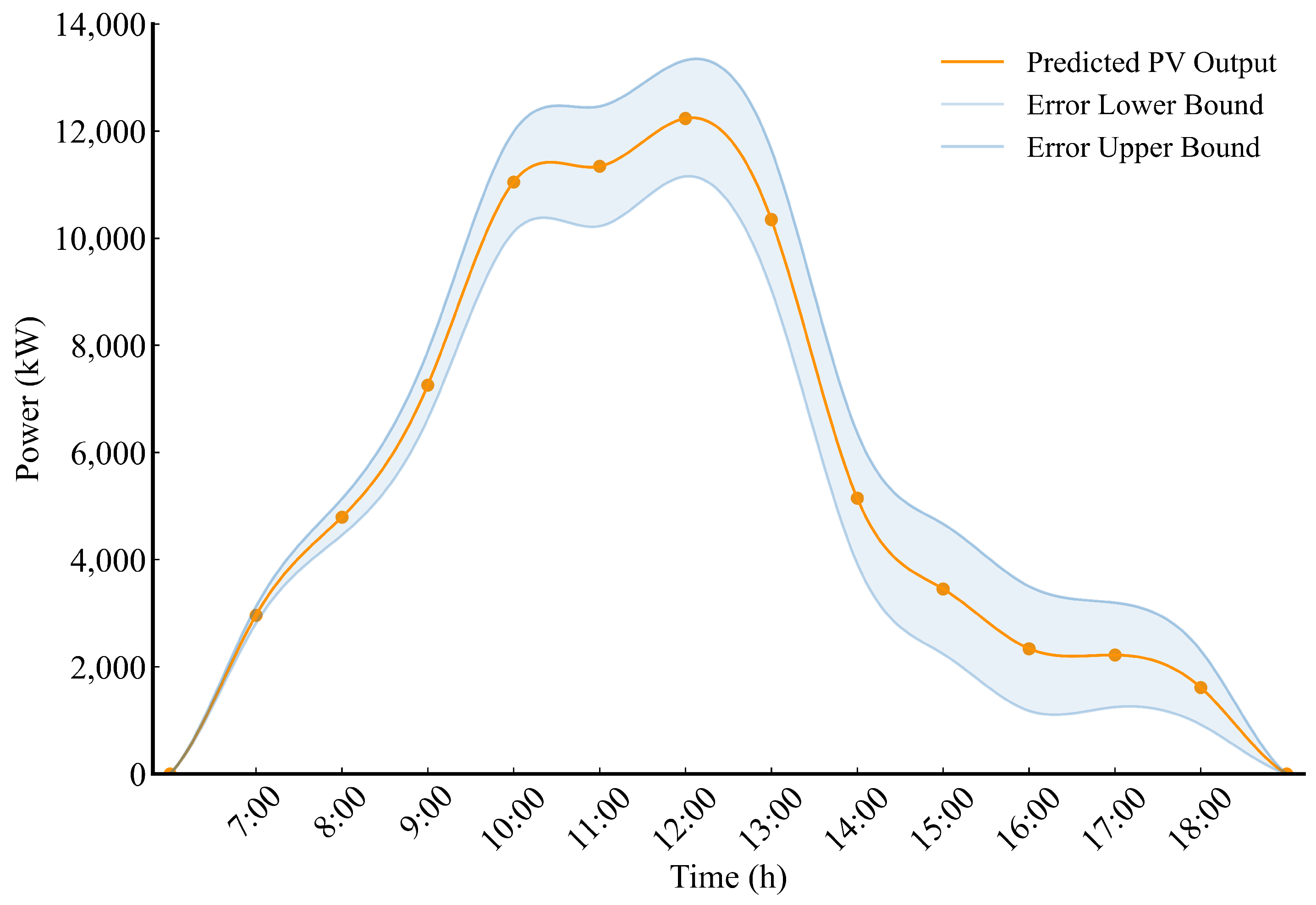
2.4.1. Uncertainty in DG Output

The actual output (${\tilde{P}}_t^{\mathrm{DG}}$) of the user’s DG can be expressed as the sum of the predicted output ($P_t^{\mathrm{pred}}$) and the deviation (${\tilde{\delta }}_t$) between the forecast and actual output.

$${\tilde{P}}_t^{\mathrm{DG}}=P_t^{\mathrm{pred}}+{\tilde{\delta }}_t$$

(3)

The uncertainty in users’ DG output is represented by an empirical distribution derived from historical forecast error data. This empirical distribution of prediction errors, denoted as $P_{\mathrm{E}}$, is constructed from r independent error vectors ${\left\{{\widehat{\delta }}_i\right\}}_{i=1}^r$. As the number of error vectors increases (i.e., as $r\to \infty$), the empirical distribution converges to the true distribution $\tilde{P}$. Here, $d_{{\widehat{\delta }}_i}$ denotes the Dirac measure associated with each ${\widehat{\delta }}_i$.

$$P_{\mathrm{E}}={\displaystyle \frac{1}{r}}\sum _{i=1}^r{d}_{{\widehat{\delta }}_i}$$

(4)

Due to the significant influence of external factors like weather, DG output is highly uncertain, which limits the accuracy of probability distribution descriptions based solely on historical data. To manage this uncertainty, the Wasserstein distance is employed to quantify the discrepancy between the empirical distribution and the true distribution of prediction errors. The Wasserstein distance [18] is defined as follows:

$$W\left(P_{\mathrm{E}},\tilde{P}\right)=\inf \left\{\underset{{\mathsf{\Xi }}^2}{\int }\parallel \widehat{\delta }-\tilde{\delta }\parallel \Pi \left(d\widehat{\delta },d\tilde{\delta }\right)\right\}$$

(5)

where, “inf” represents the infimum; $\mathsf{\Xi }$ denotes the data-driven support set; $\parallel ·\parallel$ refers to the $L^1$ norm; and $\mathsf{\Pi }$ is the joint distribution with $\widehat{\delta }$ and $\tilde{\delta }$ as the marginal distributions. Based on the Wasserstein distance, the uncertainty set $\mathcal{U}$ for DG output can be expressed as follows:

$$\mathcal{U}=\left\{\tilde{P}\in Q\left(\mathsf{\Xi }\right)\left|W\left(P_{\mathrm{E}},\tilde{P}\right)<\omega \left(r\right)\right.\right\}$$

(6)

$Q\left(\mathsf{\Xi }\right)$ represents all probability distributions within the data-driven support set. The uncertainty set is constructed as a Wasserstein ball, centered around the empirical distribution with radius $\omega \left(r\right)$. This parameter signifies the probabilistic distance to the closest accurate or most likely distribution at a given confidence level.

2.4.2. Uncertainty of Awarded Capacity in DR

According to the “Jiangsu Province Electric Power Demand Response Implementation Rules (Revised Edition)”, if the confirmed response load fails to meet the regulation target within four hours of the scheduled response time during a recent day-ahead demand response event, the power grid company will initiate an intra-day DR [19]. In this paper, EIEs are considered resources for intra-day DR. Due to considerations such as employee shift schedules and inventory management constraints, the production electricity plan is generally finalized a day in advance. Consequently, for EIEs, the awarded capacity in intra-day demand response is treated as a random variable subject to uncertainty.

Based on historical data, this paper models the awarded capacity for DR as a random variable with a normal distribution. Probability constraints are applied to the model to address the uncertainty in the awarded capacity.

$$P_r\left\{0\le {\xi }_t\le {\xi }_t^s\right\}\ge 1-\rho$$

(7)

$${\xi }_t={\displaystyle \frac{P_t^{\mathrm{bid}}}{P_t^{\mathrm{CBL}}}}$$

(8)

where the variable ${\xi }_t$ is defined as the ratio of the actual awarded capacity $P_t^{\mathrm{bid}}$ to the customer baseline load $P_t^{\mathrm{CBL}}$, with a confidence level of $1-\rho$. The probabilistic constraints above specify the confidence level at which the user’s awarded demand response capacity falls within the confidence interval $[0,{\xi }_t^s]$.

2.5. Two-Stage Distributionally Robust Optimization

This section presents the objective function and constraints of the two-stage DRO, as described below.

2.5.1. Objective Function

Following the actual production protocols of EIEs, the production electricity plan is divided into two stages: day-ahead pre-dispatch and intra-day re-dispatch. Taking into account the worst-case scenario for distributed power supply prediction errors, modeled using a Wasserstein ambiguity set, the objective is to minimize the sum of the day-ahead pre-dispatch cost ${\mathit{f}}^{\mathrm{T}}\mathit{x}$ and the expected intra-day re-dispatch cost ${\mathbb{E}}_{\tilde{P}}\left[Y\left(\mathit{x},\tilde{\delta }\right)\right]$. This formulation leads to an optimal day-ahead pre-dispatch decision $\mathit{x}$, balancing economic dispatch efficiency with robustness against uncertainty.

$$\underset{\mathit{x}}{min}\left\{{\mathit{f}}^{\mathrm{T}}\mathit{x}+\underset{\tilde{P}\in \mathcal{U}}{\sup }{\mathbb{E}}_{\tilde{P}}\left[Y\left(\mathit{x},\tilde{\delta }\right)\right]\right\}$$

(9)

The day-ahead pre-dispatch cost includes the expense for electricity purchased from the grid and the revenue generated by selling surplus electricity from the user’s DG back to the grid.

$${\mathit{f}}^{\mathrm{T}}\mathit{x}=\sum _{t\in {\mathsf{\Omega }}_T}{\lambda }_t{P}_t^{\mathrm{b}}\Delta t-\sum _{t\in {\mathsf{\Omega }}_T}{\gamma }_t{P}_t^{\mathrm{s}}\Delta t$$

(10)

The variables are defined as follows: ${\lambda }_t$ denotes the day-ahead electricity purchase price for period t; ${\gamma }_t$ represents the day-ahead feed-in tariff for selling surplus electricity back to the grid; $\Delta t$ indicates the duration of a single dispatch interval; ${\mathsf{\Omega }}_T$ represents the set of all scheduling periods for an entire workday; and $P_t^{\mathrm{b}}$ and $P_t^{\mathrm{s}}$ refer to the power purchased from the grid and the power sold back to the grid, respectively.

During the intra-day period, the day-ahead pre-dispatch strategy is adjusted to accommodate changes in production plans and participation in the grid’s intra-day demand response for load reduction. This adjustment aims to mitigate the impacts of forecast errors in DG output and the uncertainty associated with the awarded capacity for participation in the grid’s intra-day DR. The intra-day adjustment costs encompass several components:

• The cost of purchasing electricity from the grid throughout the day;
• The revenue generated from selling electricity produced by the user’s DGs;
• The penalty incurred for failing to meet the awarded DR capacity ($C_t^{\mathrm{p}}$);
• The subsidy revenue earned from participating in load reduction initiatives ($R_t^{\mathrm{cut}}$).

$$Y\left(\mathit{x},\tilde{\delta }\right)=min\sum _{t\in {\mathsf{\Omega }}_T}{\lambda }_t^{in}{\tilde{P}}_t^{\mathrm{b}}\Delta t-\sum _{t\in {\mathsf{\Omega }}_T}{\gamma }_t^{in}{\tilde{P}}_t^{\mathrm{s}}\Delta t+\sum _{t\in {\mathsf{\Omega }}_{res}}{C}_t^{\mathrm{p}}-\sum _{t\in {\mathsf{\Omega }}_{res}}{R}_t^{\mathrm{cut}}$$

(11)

$$C_t^{\mathrm{p}}=max\left\{\beta \left(R_1{\xi }_t{P}_t^{\mathrm{CBL}}-P_t^{\mathrm{cut}}\right),0\right\}$$

(12)

$$P_t^{\mathrm{cut}}=P_t^{\mathrm{CBL}}-{\tilde{P}}_t^{\mathrm{b}}$$

(13)

$$R_t^{\mathrm{cut}}=\left\{\begin{array}{c}0,P_t^{\mathrm{cut}}<R_1{\xi }_t{P}_t^{\mathrm{CBL}}\hfill \\ D_1\pi P_t^{\mathrm{cut}},R_1{\xi }_t{P}_t^{\mathrm{CBL}}\le P_t^{\mathrm{cut}}<R_2{\xi }_t{P}_t^{\mathrm{CBL}}\hfill \\ D_2\pi P_t^{\mathrm{cut}},R_2{\xi }_t{P}_t^{\mathrm{CBL}}\le P_t^{\mathrm{cut}}<R_3{\xi }_t{P}_t^{\mathrm{CBL}}\hfill \\ D_3\pi {\xi }_t{P}_t^{\mathrm{CBL}},P_t^{\mathrm{cut}}\ge R_3{\xi }_t{P}_t^{\mathrm{CBL}}\hfill \end{array}\right.$$

(14)

where ${\mathsf{\Omega }}_{res}$ represents the set of intra-day demand response periods; ${\lambda }_t^{in}$ and ${\gamma }_t^{in}$ denote the purchase and sale prices during the intra-day period, respectively; $\pi$ is the subsidy rate for load reduction in the intra-day demand response; $\beta$ is the penalty factor for failing to meet the response capacity target; $R_1,R_2$ and $R_3$ are the response threshold ratios; and $D_1,D_2$ and $D_3$ represent the response capacity discount factors, respectively.

The customer baseline load $P_t^{\mathrm{CBL}}$ is computed as follows:

$$P_t^{\mathrm{CBL}}={\displaystyle \frac{1}{n}}\sum _{D=d-n}^{d-1}{P}_t^{\mathrm{b},D}$$

(15)

where $P_t^{b,D}$ denotes the electricity purchase power from the main grid on the day D before the response day d, and n represents the number of selected load samples.

2.5.2. Constraints

• Single Operational State for Task Nodes

For task j, there is only one operational mode at any given time t.

$$\left\{\begin{array}{c}0\le {\displaystyle \sum _{k\in K_j}}{Z}_{j,k,t}\le 1\hfill \\ Z_{j,k,t}\in \{0,1\}\hfill \end{array}\right.$$

(16)

In this equation, $Z_{j,k,t}$ represents a binary state variable indicating the operational mode of task j. When $Z_{j,k,t}=1$, it signifies that task j is operating in mode k at time t. Furthermore, $K_j$ denotes the set of all possible operating modes for task j.

• Material Balance

$$S_{t+1}^i=S_t^i+\left(\sum _{j\in G_i}\sum _{k\in K_j}{g}_{i,j,k}{Z}_{j,k,t}-\sum _{j\in C_i}\sum _{k\in K_j}{c}_{i,j,k}{Z}_{j,k,t}\right)\Delta t$$

(17)

Here, $S_t^i$ denotes the material inventory at state node i at time t; $G_i$ and $C_i$ represent the sets of tasks associated with state node i that produce and consume material i, respectively. Additionally, $g_{i,j,k}$ and $c_{i,j,k}$ are the production and consumption rates of material i for task j at state node i when task j operates in mode k.

• Material Storage

$$S_i^{min}\le S_t^i\le S_i^{max}$$

(18)

In this equation, $S_i^{min}$ and $S_i^{max}$ are the lower and upper material inventory limits for state node i, respectively.

• Target Output of Final Product

$$S_{T-1}^{\mathrm{f}}-S_0^{\mathrm{f}}\ge S_{\mathrm{sta}}^{\mathrm{f}}$$

(19)

where $S_{\mathrm{sta}}^{\mathrm{f}}$ represents the target daily output of the final product.

• Continuity of Operational Modes for Task Nodes

Since equipment operation status cannot be modified within a single cycle for adjustable task nodes, this paper establishes a minimum operational duration requirement for task j. Specifically, task j must remain in a fixed mode for the duration of each cycle, with the minimum duration defined by the task’s minimum production cycle. For instance, if the minimum production cycle for a task is 2 h, $T_{j,min}^{\mathrm{on}}$ is set to 2 h.

$$\left(T_{j,t-1}^{\mathrm{on}}-T_{j,min}^{\mathrm{on}}\right)\left(Z_{j,k,t-1}-Z_{j,k,t}\right)\ge 0$$

(20)

The non-adjustable task node maintains a fixed operational state throughout the scheduling day.

$$Z_{j,k,t}=Z_{j,0,t}$$

(21)

where $Z_{j,0,t}$ represents the task node in a specific operational mode.

• Electricity Purchase or Sale

$$\begin{array}{c}\hfill I_t^{\mathrm{b}}{P}^{\mathrm{b},min}\le P_t^{\mathrm{b}}\le I_t^{\mathrm{b}}{P}^{\mathrm{b},max}\end{array}$$

(22)

$$\begin{array}{c}\hfill I_t^{\mathrm{s}}{P}^{\mathrm{s},min}\le P_t^{\mathrm{s}}\le I_t^{\mathrm{s}}{P}^{\mathrm{s},max}\end{array}$$

(23)

$$\left\{\begin{array}{c}{I}_t^{\mathrm{b}}+I_t^{\mathrm{s}}\le 1\hfill \\ I_t^{\mathrm{b}},I_t^{\mathrm{s}}\in \{0,1\}\hfill \end{array}\right.$$

(24)

Here, $P^{\mathrm{b},max}$ and $P^{\mathrm{b},min}$ represent the maximum and minimum limits on power purchased by industrial users from the main grid, respectively, while $P^{\mathrm{s},max}$ and $P^{\mathrm{s},min}$ indicate the upper and lower limits on power sold back to the grid. The binary variables $I_t^{\mathrm{b}}$ and $I_t^{\mathrm{s}}$ signify the status of power purchase or sale: when $I_t^{\mathrm{b}}=1$, power is being purchased, and when $I_t^{\mathrm{s}}=1$, power is being sold. To align with the “self-generation for self-consumption, with surplus power fed into the grid” business model, these variables cannot equal one simultaneously.

• Power Balance

$$\left\{\begin{array}{c}{P}_t^{\mathrm{b}}+P_t^{\mathrm{pred}}=P_t^{\mathrm{STN}}+P_t^{\mathrm{s}}\hfill \\ P_t^{\mathrm{STN}}={\displaystyle \sum _{j=1}^m}{P}_{j,t}\hfill \\ P_{j,t}={\displaystyle \sum _{k\in K_j}}{Z}_{j,k,t}{P}_{j,k}\hfill \end{array}\right.$$

(25)

In these equations, $P_t^{\mathrm{STN}}$ denotes the total power consumption across all task nodes within the STN model, where m represents the total number of task nodes. Here, $P_{j,t}$ indicates the electrical power consumption of task j at time t, while $P_{j,k}$ specifies the power usage of task j when operating in mode k.

2.6. Model Reconstruction and Transformation

2.6.1. Constraint Adjustment

Building on the day-ahead pre-dispatch plan, users can implement intra-day readjustments by flexibly modifying the power they purchase or sell. These adjustments aim to correct for forecast errors in DG output from the prior day. This paper employs an affine adjustment strategy, as presented in [20,21]. Under this approach, an affine factor $a_t$ is introduced, allowing the intra-day adjustment decision $y_t$ to be expressed as a linear function of the forecast error, represented by the random variable ${\tilde{\delta }}_t$.

$$y_t\left({\tilde{\delta }}_t\right)=x_t+a_t{\tilde{\delta }}_t$$

(26)

The affine strategy provides a way to transform the problem into a computationally feasible and physically interpretable equivalent model. This approach enables users to adjust their electricity consumption strategies in response to forecast errors, guided by the affine factor. The specific constraints for these adjustments are outlined as follows:

• Electricity Purchase or Sale Adjustment

$$\left\{\begin{array}{c}{\tilde{P}}_t^{\mathrm{b}}=P_t^{\mathrm{b}}+a_t^{\mathrm{b}}{\tilde{\delta }}_t\hfill \\ {\tilde{P}}_t^{\mathrm{s}}=P_t^{\mathrm{s}}+a_t^{\mathrm{s}}{\tilde{\delta }}_t\hfill \end{array}\right.$$

(27)

• Power Balance Adjustment

$$\left\{\begin{array}{c}{\tilde{P}}_t^{\mathrm{STN}}={\displaystyle \sum _{j=1}^m}{P}_{j,t}+a_{j,t}{\tilde{\delta }}_t\hfill \\ a_t^{\mathrm{b}}{\tilde{\delta }}_t+{\tilde{\delta }}_t={\displaystyle \sum _{j=1}^m}{a}_{j,t}{\tilde{\delta }}_t+a_t^{\mathrm{s}}{\tilde{\delta }}_t\hfill \end{array}\right.$$

(28)

These equations outline the adjustment strategies and constraints that should be implemented to address DG prediction errors. By introducing affine factors $a_t^{\mathrm{b}}$, $a_t^{\mathrm{s}}$, and $a_{j,t}$, the purchased power, sold power, and production load are adjusted to ${\tilde{P}}_t^{\mathrm{b}}$, ${\tilde{P}}_t^{\mathrm{s}}$ and ${\tilde{P}}_t^{\mathrm{STN}}$, respectively.

2.6.2. Probability Constraint Transformation

To address the probability constraints in the model, it can be approximated using scenario sampling, thereby transforming it into a scenario-based MILP problem for more efficient resolution. Given the probability density distribution of the user’s DR capacity, Latin hypercube sampling [22] is employed to generate N samples. When the sample size N is sufficiently large, the probability constraints can be approximated using a bilinear form, enabling the probability constraints in Equation (7) to be equivalently represented as mixed-integer linear constraints, as shown in the following equation.

$$\left\{\begin{array}{c}\left({\xi }_t-{\xi }_t^s\right)\left(1-z_s\right)\le 0\hfill \\ {\displaystyle \sum _s}{z}_s\le \rho N\hfill \\ z_s\in \{0,1\}s=1,2\dots ,N\hfill \end{array}\right.$$

(29)

In the equation, $z_s$ is a binary variable. When $z_s=1$, the corresponding scenario is excluded; conversely, when $z_s=0$, the chance constraint is satisfied. The confidence level of the original probability constraint can be approximated by counting the number of scenarios where $z_s=0$. Compared to the Big-M formulation for converting the probability constraint, the bilinear form approach described above enables the relaxation of the entire constraint by setting the scenario state variable to 1. This method reduces the problem size and improves computational efficiency.

2.6.3. Transformation of DRO

For a more straightforward presentation, the DRO model in Equation (9) is reformulated into the following compact matrix form:

$$\left\{\begin{array}{c}{\displaystyle \underset{\mathit{x}}{min}}\left\{{\mathit{f}}^{\mathrm{T}}\mathit{x}+\underset{\tilde{P}\in \psi }{\sup }{\mathbb{E}}_{\tilde{P}}\left[min{\mathit{h}}^{\mathrm{T}}\mathit{y}\left(\mathit{x},\tilde{\delta }\right)\right]\right\}\hfill \\ \mathrm{s}.\mathrm{t}.\mathit{Ax}\le \mathit{b}\hfill \\ \mathit{Gy}\left(\mathit{x},\tilde{\delta }\right)\le \mathit{e}\left(\tilde{\delta }\right)\hfill \end{array}\right.$$

(30)

where ${\mathit{h}}^{\mathrm{T}}\mathit{y}$ denotes the objective function of the second stage.

Based on the Slater condition [23], it can be concluded that the original model satisfies strong duality. Therefore, the intra-day rescheduling model can be reformulated by leveraging the principle of strong duality.

$$\underset{\tilde{P}\in \psi }{\sup }{\mathbb{E}}_{\tilde{P}}\left[min{\mathit{h}}^{\mathrm{T}}\mathit{y}\left(\mathit{x},\tilde{\delta }\right)\right]=\underset{\alpha \ge 0}{inf}\{\alpha \omega \left(r\right)+{\displaystyle \frac{1}{r}}\sum _{i=1}^r\underset{\tilde{\delta }\in \mathsf{\Xi }}{sup}({\mathit{h}}^{\mathrm{T}}\mathit{y}(\mathit{x},\tilde{\delta })-\alpha ∥\tilde{\delta }-{\widehat{\delta }}_i∥)\}$$

(31)

In the equation, $\alpha$ denotes the dual variable, while ${\widehat{\delta }}_i$ represents the i-th error sampling point. Equation (31) can be reformulated as follows:

$$\left\{\begin{array}{c}\underset{\alpha \ge 0}{inf}(\alpha \omega \left(r\right)+{\displaystyle \frac{1}{r}}{\displaystyle \sum _{i=1}^r}{\tau }_i)\hfill \\ \mathrm{s}.\mathrm{t}.\underset{\tilde{\delta }\in \mathsf{\Xi }}{sup}({\mathit{h}}^{\mathrm{T}}\mathit{y}(\mathit{x},\tilde{\delta })-\alpha ∥\tilde{\delta }-{\widehat{\delta }}_i∥)\le {\tau }_i\hfill \end{array}\right.$$

(32)

where ${\tau }_i$ represents the auxiliary variable.

The original model is constrained by infinite constraints, classifying it as a semi-infinite programming problem, which is inherently difficult to solve directly. To address computational challenges, an approximation model is introduced. By applying the affine strategy during the intra-day rescheduling stage, the inner and outer minimization problems are combined, resulting in a two-level optimal scheduling model formulated as a min-max problem. The final DRO model framework is then derived by consolidating the formulations from the first stage.

$$\left\{\begin{array}{cc}\hfill & \underset{\mathit{x},\alpha }{min}{\mathit{f}}^{\mathrm{T}}\mathit{x}+\alpha \omega \left(r\right)+{\displaystyle \frac{1}{r}}\sum _{i=1}^r{\tau }_i\hfill \\ \hfill & \mathrm{s}.\mathrm{t}.\mathit{A}\mathit{x}\le \mathit{b}\hfill \\ \hfill & \alpha \ge 0\hfill \\ \hfill & {\mathit{h}}^{\mathrm{T}}\mathit{y}(\mathit{x},{\tilde{\delta }}_i)\le {\tau }_i\hfill \\ \hfill & {\mathit{h}}^{\mathrm{T}}\mathit{y}(\mathit{x},\overline{\widehat{\delta }})-\alpha \parallel \overline{\widehat{\delta }}-{\widehat{\delta }}_i\parallel \le {\tau }_i\hfill \\ \hfill & {\mathit{h}}^{\mathrm{T}}\mathit{y}(\mathit{x},\underset{¯}{\overset{^}{\delta }})-\alpha \parallel \underset{¯}{\overset{^}{\delta }}-{\widehat{\delta }}_i\parallel \le {\tau }_i\hfill \\ \hfill & \mathit{G}\mathit{y}(\mathit{x},\overline{\widehat{\delta }})\le \mathit{e}(\overline{\widehat{\delta }})\hfill \\ \hfill & \mathit{G}\mathit{y}(\mathit{x},\underset{¯}{\overset{^}{\delta }})\le \mathit{e}\left(\underset{¯}{\overset{^}{\delta }}\right)\hfill \end{array}\right.$$

(33)

In Equation (33), $\overline{\widehat{\delta }}$ and $\underset{¯}{\overset{^}{\delta }}$ represent the upper and lower bounds of the forecast error, respectively. Applying this transformation, the original two-stage DRO objective function, formulated initially to address the worst-case expectation problem, is reformulated as a linear optimization problem involving an auxiliary variable $\alpha$. This reformulation allows the use of commercial solvers, thereby enhancing the computational efficiency of the model.

3. Case Study

This example examines a cement plant in western China with an annual production capacity of 14 million tons. The plant is a case study for applying a two-stage DRO dispatch model to optimize its daily (24 h) electricity consumption. As an EIE, the plant participates in the electricity market through a dual-payment system, which includes both day-ahead and intra-day stages.

3.1. Parameters

The intra-day purchase and sale prices may vary by ±30% relative to the day-ahead prices presented in

Table 1. Electricity parameters for the cement plant.

Parameter	Value
Peak Hour 1 Purchase Electricity Price $\left({\lambda }_t\right)$	0.8248 CNY/kWh
Peak Hour Sale Electricity Price $\left({\gamma }_t\right)$	0.6186 CNY/kWh
Normal Hour 2 Purchase Electricity Price $\left({\lambda }_t\right)$	0.5499 CNY/kWh
Normal Hour Sale Electricity Price $\left({\gamma }_t\right)$	0.4124 CNY/kWh
Off-Peak Hour 3 Purchase Electricity Price $\left({\lambda }_t\right)$	0.2749 CNY/kWh
Off-Peak Hour Sale Electricity Price $\left({\gamma }_t\right)$	0.2062 CNY/kWh
Penalty Factor for Not Meeting DR Target $\left(\beta \right)$	4.0 CNY/kWh
Subsidy Rate for Load Reduction $\left(\pi \right)$	3.0 CNY/kWh
DR Threshold Ratios $(R_1,R_2,R_3)$	50%/70%/120%
DR Capacity Discount Factors $(D_1,D_2,D_3)$	60%/100%/120%
Installed Capacity of DGs	14 MW
Upper Limits of Power Purchased $\left(P^{b,max}\right)$	15,000 kW
Upper Limits of Power Sold $\left(P^{s,max}\right)$	10,000 kW

¹ 9:00–12:00, 17:00–22:00. ² 7:00–9:00, 12:00–17:00, 22:00–23:00. ³ 0:00–7:00, 23:00–24:00.

. The cement plant’s production process, represented by the STN model in Figure 4, includes three task nodes and four state nodes. Among these, the raw material grinding and cement milling processes are classified as adjustable task nodes, with 2 h and 1 h durations. The clinker calcination process is considered a non-adjustable task node to ensure production safety and minimize significant heat losses during start-stop operations. As a result, both the shaft and rotary kiln must operate in a fixed state throughout the entire scheduling period. The parameters for the STN nodes are provided in

Table 2. Attributes of STN state nodes.

Material *	Storage Upper Limit (tons) ${\mathit{S}}_{\mathit{i}}^{\mathit{max}}$	Storage Lower Limit (tons) ${\mathit{S}}_{\mathit{i}}^{\mathit{min}}$	Initial Value (tons) ${\mathit{S}}_{\mathit{i}}^0$
S1	10,000	0	8000
S2	2000	0	0
S3	5000	0	0
S4	10,000	0	0

* S1: Raw Material (i = 1), S2: Raw Meal (i = 2), S3: Clinker (i = 3), S4: Cement Product (i = 4).

and

Table 3. Attributes of STN task nodes.

Task *	Operating Mode k	Material Consumption Rate (tons/h) ${\mathit{c}}_{\mathit{i},\mathit{j},\mathit{k}}$	Product Output Rate (tons/h) ${\mathit{g}}_{\mathit{i},\mathit{j},\mathit{k}}$	Power Consumption (kW) ${\mathit{P}}_{\mathit{j},\mathit{k}}$
	1	0	0	0
T1	2	320	300	3000
	3	400	350	4500
T2	1	280	250	1900
	1	0	0	0
T3	2	160	150	4000
	3	240	220	6500

* T1: Raw Material Grinding (j = 1), T2: Clinker Calcination (j = 2), T3: Cement Milling (j = 3).

.

3.2. Dataset

Data were gathered from a publicly available source at various time points during 24 h, using the day-ahead forecast error dataset for photovoltaic (PV) systems provided by the Belgian grid operator, Elia [24]. Original data are scaled by a specified percentage to match the cement plant’s load profile. Figure 5 illustrates the predicted output ($P_t^{\mathrm{pred}}$) and the deviation (${\tilde{\delta }}_t$) data. Notably, during the time period from 19:00 to 06:00 the following day, the photovoltaic output is nearly zero; therefore, this period is not displayed in the figure. It is important to note that this approach serves as a convenient data collection method. In real EIE scenarios, there would also be substantial historical forecasting error data available internally. Furthermore, to account for the uncertainty associated with the awarded capacity of intra-day demand response participants, Latin hypercube sampling is used to generate 2000 samples of the awarded capacities.

This paper defines the scheduling day as the period from 00:00 on the current day to 00:00 on the following day. A discrete-time model is used for the analysis, dividing the day into n equal time intervals, each with a duration of $\Delta t$. The state parameters are assumed to remain constant for each period. For this study, the scheduling interval is set to one hour.

4. Results

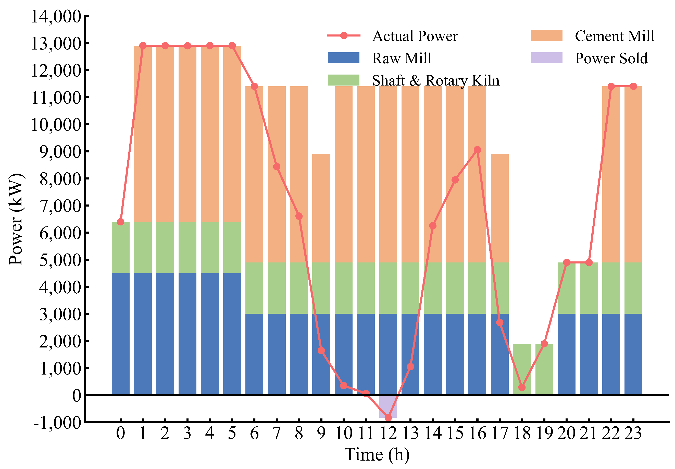
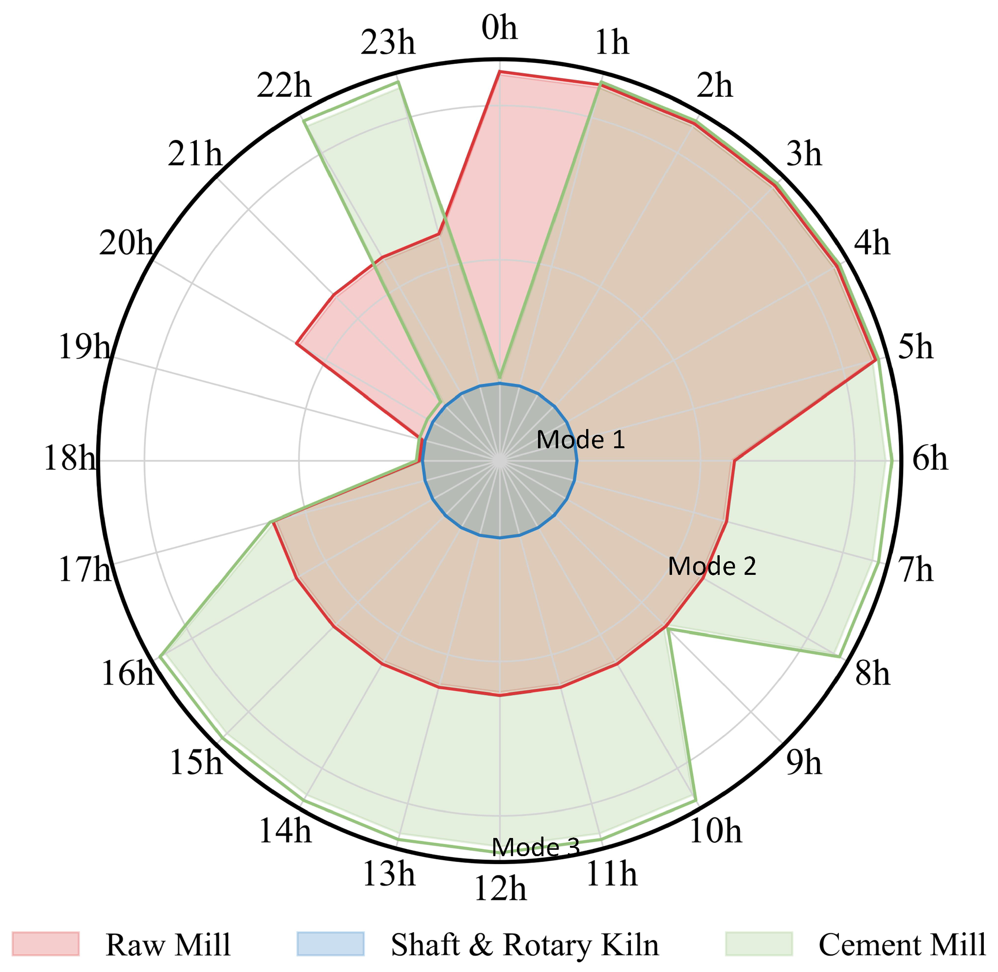
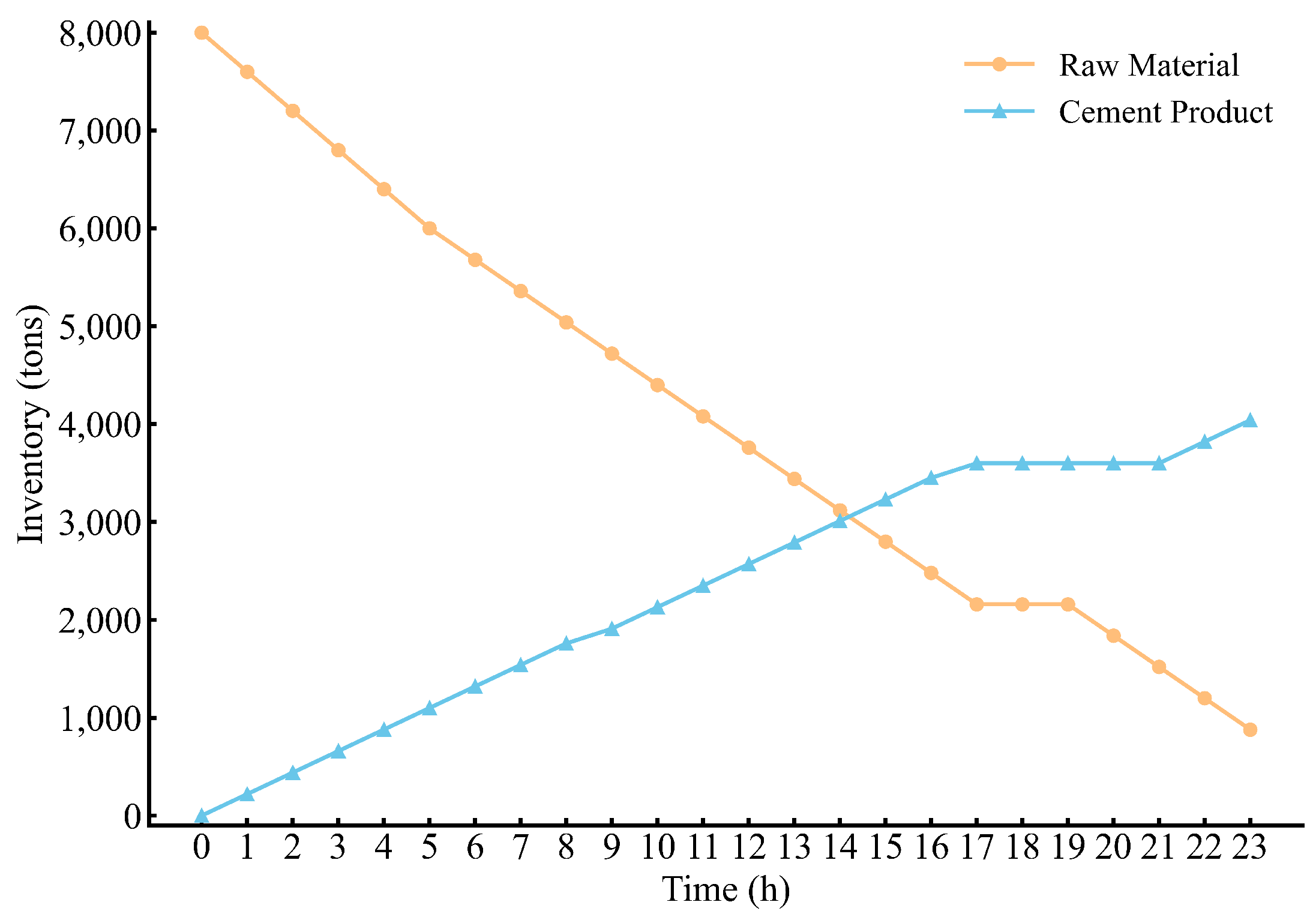
4.1. Strategy Analysis

It is important to note that the result of the two-stage DRO optimization represents a pre-scheduling decision. This is due to the application of an affine strategy, which transforms the intra-day rescheduling decision into a function of the prediction error associated with the DG.

Figure 6 provides an overview of the pre-dispatch strategy of the cement plant. During periods of low electricity prices (e.g., 1:00–7:00), the plant purchases a significant amount of electricity, primarily driven by the peak-valley price differential. In contrast, electricity purchases are reduced during periods of higher photovoltaic (PV) output, particularly between 9:00 and 14:00. Additionally, during peak demand periods on the main grid (18:00–20:00), the plant’s electricity purchases remain relatively low. The maximum production capacity of the cement plant ($P_t^{\mathrm{STN}}$) is 12,900 kW. When the PV output exceeds this capacity during the midday period (12:00–13:00), the plant exports 836 kW of surplus power back to the grid.

Furthermore, as shown in Figure 7, the user adjusts the electrical load by modifying the operating modes of the production equipment in response to price signals or demand response signals. In particular, during the load shedding period (18:00–20:00) in the intra-day demand response, the raw and cement mills operate in Mode 1 (shutdown). After the demand response period, the raw mill resumes normal production earlier than the cement mill. Analysis indicates that this occurs because, in the period leading up to the demand response (10:00–16:00), the cement mill continuously operates in Mode 3 (high power), remaining in a normal production state at the end of the demand response period. Consequently, this leads to a low inventory of cement, which requires the cement mill to wait for the preceding production to catch up.

As can be seen in Figure 8, during a one-day production scheduling cycle, the raw material stock decreases from 8000 tons to 880 tons. The final cement production reaches 4040 tons, consistent with the daily target of 4000 tons.

DRO combines the features of both stochastic and robust optimization. The radius of the Wasserstein ball, defined within an uncertainty set based on the Wasserstein distance, reflects the risk appetite in DRO [25]. As shown in Equation (34), this radius is influenced by the number of sample prediction errors. To evaluate the effect of sample size on risk appetite in decision-making, a simulation analysis of scheduling costs is performed by varying the number of samples. The results of the analysis can be compared in

Table 4. Comparison of costs for different sample sizes.

Sample Size	Day-Ahead Pre-Dispatch Cost (CNY)	Intra-Day Re-Dispatch Cost (CNY)	Total Cost (CNY)	Solution Time (s)
100	72,213	43,273	115,486	28.12
150	72,048	43,374	115,422	39.06
200	71,938	43,454	115,392	56.50
250	72,075	43,321	115,396	65.62
300	71,526	43,701	115,227	78.75
350	70,426	44,431	114,857	91.68

.

$$\left\{\begin{array}{c}\omega \left(r\right)=C_w\sqrt{{\displaystyle \frac{1}{r}}ln{\displaystyle \frac{1}{1-\theta }}}\hfill \\ C_w\approx 2{\displaystyle \underset{\eta >0}{inf}}\sqrt{{\displaystyle \frac{1}{2\eta }}\left[1+ln\left({\displaystyle \frac{1}{r}}{\displaystyle \sum _{i=1}^r}{e}^{\eta \parallel {\widehat{\delta }}_i-\overline{\mu }{\parallel }^2}\right)\right]}\hfill \end{array}\right.$$

(34)

where $\theta$ is the confidence level of the uncertainty set, $\overline{\mu }$ denotes the average of the historical day-ahead forecast error dataset for PV output.

The results in Table 4 show that with a small sample size of historical PV day-ahead forecast errors, the radius of the Wasserstein ball is relatively large. This leads to a conservative day-ahead pre-dispatch strategy, as the uncertainty set encompasses a wide range of potential probability distributions, resulting in less economically favorable outcomes. As the sample size increases, the radius of the uncertainty set becomes smaller, allowing for a more accurate representation of the probability distribution of uncertain variables, thereby better approximating the actual distribution. The increase in sample size essentially reduces the conservativeness of the pre-scheduling strategy, improving its economic performance and ultimately affecting the total cost. As a result, the dispatch strategy becomes more economically efficient.

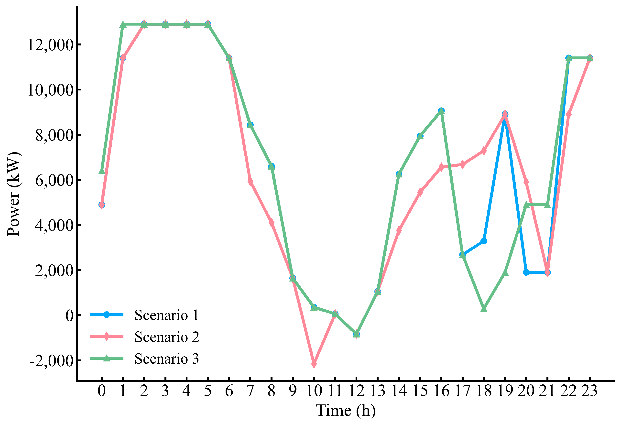
4.2. Comparison of Different Scenarios

Based on user participation in DR and timing, assuming a sample size of 350 for PV day-ahead forecast errors and a daily output target of 4000 tons of final cement products, the following three scenarios are established for comparative simulation.

• Scenario 1: No participation in intra-day invited DR.
• Scenario 2: Participation in intra-day invited DR from 10:00 to 12:00.
• Scenario 3: Participation in intra-day invited DR from 18:00 to 20:00.

As shown in

Table 5. Comparison of costs across different scenarios.

Scenario ID	Day-Ahead Pre-Dispatch Cost (CNY)	Intra-Day Re-Dispatch Cost (CNY)	Total Cost (CNY)
1	69,602	89,277	158,879
2	69,632	80,152	149,784
3	70,426	44,431	114,857

, among these scenarios, Scenario 3 has the lowest total cost to users. Specifically, the total cost in Scenario 3 is reduced by CNY 44,022 or 27.7%, compared to Scenario 1. In contrast, the cost in scenario 2 is reduced by only CNY 9095 or 5%, relative to scenario 1. These results suggest that the participation of EIEs in the grid’s intra-day invited DR program leads to a substantial reduction in operating costs. Furthermore, participation during the evening hours of the DR period has a more pronounced effect. Taking Scenario 1 as the baseline, an analysis of the data presented in Figure 9 reveals the following.

In Scenario 2 (DR program 10:00–12:00), the DR effect is mainly observed at 10:00, where the EIE delivers 2148.95 kW of power to the upper-level grid, in contrast to Scenario 1, where 351.05 kW of power is purchased from the grid during this period. However, during the 11:00 and 12:00 periods, the curves for Scenario 2 and Scenario 1 overlap. This is primarily because the user’s photovoltaic (PV) output during these periods is substantial, enabling full self-consumption with the surplus power being fed into the grid. Consequently, the baseline load during this period is relatively low. For instance, at 11:00, the baseline load in Scenario 1 is only 59.74 kW, rendering the DR penalty costs for EIE users less sensitive in this time frame.

In Scenario 3 (DR program 18:00–20:00), the impact of EIE participation in the DR program is notably significant. From the perspective of overall load reduction, Scenario 3 achieves a total load reduction of 7000 kW compared to Scenario 1. Specifically, at 18:00 and 19:00, Scenario 3 reduces the load by 3000 kW and 7000 kW, respectively, relative to Scenario 1. However, at 20:00, the load in Scenario 3 exceeds that of Scenario 1 by 3000 kW. This can be attributed to the substantial load reductions in the preceding two periods. Given that only four hours remain until the end of the production day, meeting the day’s production targets becomes a priority. To fulfill these constraints, the system compromises by increasing the load at 20:00 to ensure that daily production goals are achieved.

Additionally, comparing dispatch costs between the day-ahead and intra-day phases across all three scenarios reveals that intra-day phase costs are generally higher. This is primarily due to the need for adjustments in purchased or sold power during the intra-day phase to address day-ahead forecast errors in PV output. The electricity prices for power purchases or sales during the intra-day phase are typically more favorable or less favorable than those in the day-ahead phase, leading to an overall increase in costs during the intra-day phase.

Compared to Scenario 2, Scenario 3 has a more significant impact on reducing the total cost for the user. This is because the DR period in Scenario 2 is set between 10:00 and 12:00, when power demand is already relatively low. As shown in Figure 9, the power is negative at 10:00 and 12:00, indicating that power is being sold back to the grid during these times.

The capacity for load reduction among EIEs participating in intra-day DR is primarily determined by the actual output of DGs, which directly influences the potential for cost reduction. When DG output exceeds the previous day’s forecast, the potential for load reduction increases, thereby lowering costs. However, when the actual output is below the forecast, the effect on cost reduction is less significant.

4.3. DRO Algorithm Sensitivity Analysis

Cement plants often set varying daily production targets to account for seasonal fluctuations in cement sales. To assess the applicability of the model proposed in this study, five distinct production target scenarios are analyzed using stochastic optimization (SO), robust optimization (RO), and the two-stage distributionally robust optimization (DRO) method introduced here, as shown in

Table 6. Comparison of costs across different algorithms.

Algorithm	SO (CNY)	DRO (CNY)	RO (CNY)
3400	81,963	85,425	86,030
3700	96,239	100,587	101,206
4000	109,784	114,896	115,515
4300	124,106	130,067	130,692
4600	141,981	149,043	149,662

.

As shown in Figure 10, the costs associated with the DRO method consistently fall between those of SO [26] and RO [27] across different production targets for final cement products. Taking the target production of 3400 tons as an example, the RO method employs a conservative pre-scheduling strategy, resulting in higher day-ahead costs and the highest total cost of CNY 86,030. Although this method exhibits strong robustness, it significantly compromises economic efficiency. Conversely, the SO method assumes an exact probability distribution for DG output forecast errors. Consequently, the derived operational strategy underestimates intra-day power purchase costs and response deviation penalties, yielding an overly optimistic total cost of CNY 81,963. However, this approach lacks the capacity to manage risks beyond the assumed probability distribution, as it disregards intra-day uncertainties. While the SO method achieves superior economic efficiency, its robustness is notably weak. The operational strategies obtained through these two optimization methods are therefore of limited practical utility, as they fail to balance robustness and economic efficiency comprehensively. This outcome demonstrates that the proposed two-stage DRO model effectively balances economic efficiency and robustness, making it adaptable to cement plants’ fluctuating daily production requirements.

5. Discussion

It is important to note that simplifying the approach proposed in this paper to treat DR capacity as the optimization objective makes it possible to calculate the DR capability while considering the user’s economic interests. Compared to traditional methods, where the power grid relies solely on macro-level information reported by users to estimate their DR capability, this approach simulates the user’s production processes to derive DR capability, resulting in more realistic outcomes. This reduces the likelihood of conservative underreporting of DR capacity due to users’ reluctance to disrupt production schedules.

Furthermore, for EIE users, this method provides an efficient energy management strategy that ensures the economic efficiency of their production processes while participating in demand response programs. It achieves a balance between meeting grid requirements and maintaining production objectives, demonstrating broad potential for practical applications.

However, certain limitations remain before this method can be fully implemented in practice. From the perspective of grid scheduling, the model requires faster solution speeds. Currently, the solution process takes approximately 30 s, and improving the algorithm’s computational efficiency will be a focus of future research.

6. Conclusions

This paper has combined the Wasserstein uncertainty set, probability constraints, the STN model, and distributionally robust optimization to propose a two-stage DRO model for managing electricity consumption in EIEs under multiple sources of uncertainty. The model is validated through a case study of a real cement plant, leading to the following conclusions:

• This study characterizes uncertainties in DG output and the awarded capacity of intra-day invited DR using a Wasserstein distance-based uncertainty set and probability constraints. It then formulates a two-stage DRO model for day-ahead and intra-day electricity planning in EIEs. Within the framework of the STN model, the proposed approach provides an economically efficient production electricity plan that satisfies the users’ demands while offering a detailed equipment operation schedule for EIE participation in DR.
• By varying the sample size of historical forecast errors, the DRO model effectively adjusts the radius of the Wasserstein ball, striking a balance between economic efficiency and robustness in the optimization solution. This approach leverages the capacity of stochastic optimization to incorporate expected risks based on historical data while benefiting from the strong robustness characteristics of robust optimization. The participation of EIEs in intra-day invited demand response results in substantial cost reductions, with the most significant effects observed during evening demand response periods.
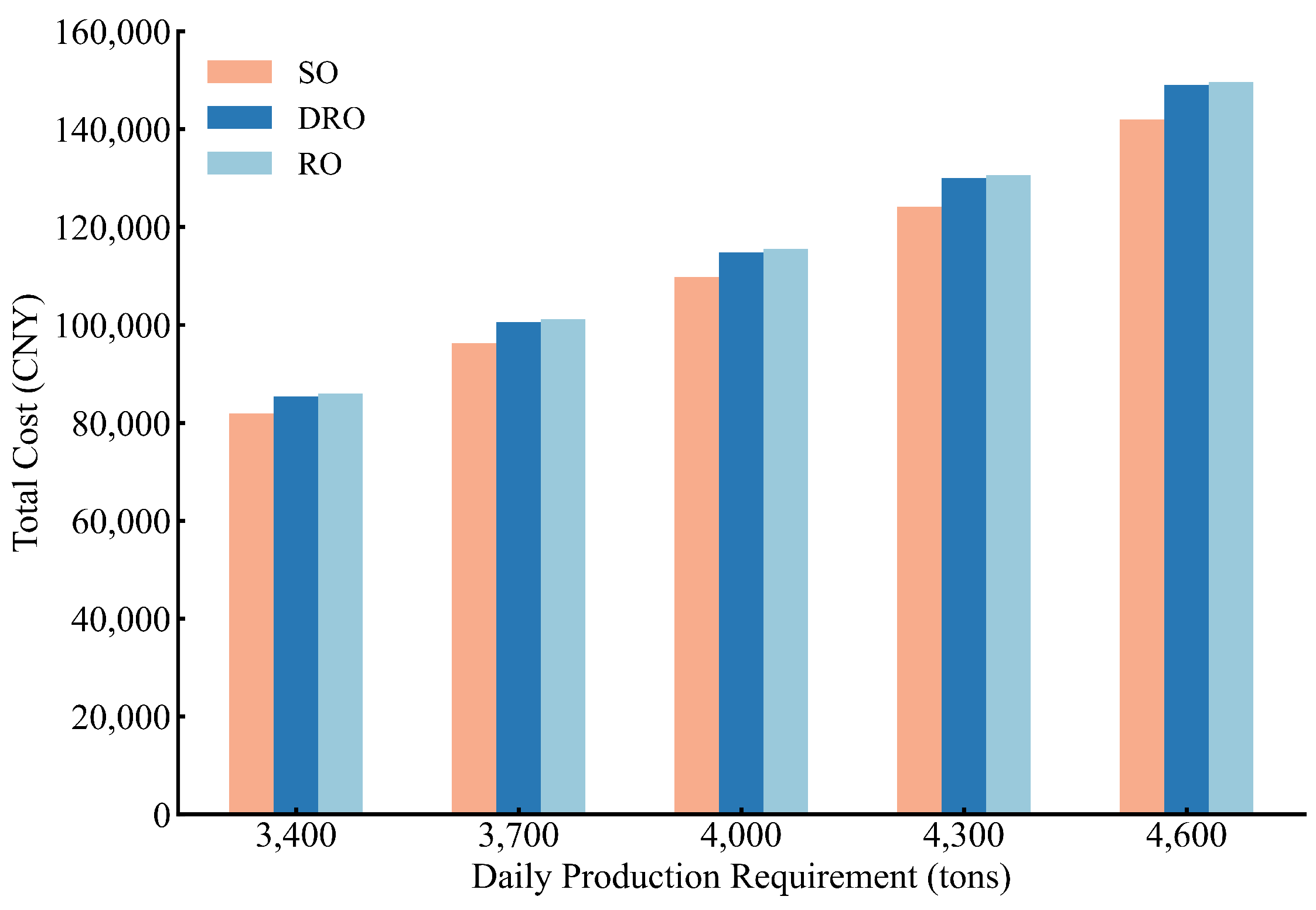
• Across varying target production levels, the scheduling costs of the DRO model consistently lie between those of SO and RO. This shows that the proposed model effectively balances economic efficiency and robustness in different scenarios, highlighting its strong generalizability.

References

1. Impram, S.; Nese, S.V.; Oral, B. Challenges of renewable energy penetration on power system flexibility: A survey. Energy Strat. Rev. 2020, 31, 100539. [Google Scholar] [CrossRef]
2. Liao, S.Y.; Xu, J.; Sun, Y.Z.; Bao, Y.; Tang, B.W. Control of Energy-Intensive Load for Power Smoothing in Wind Power Plants. IEEE Trans. Power Syst. 2018, 33, 6142–6154. [Google Scholar] [CrossRef]
3. Xu, Q.; Lin, L.; Liang, Q.M. What influences industrial enterprises’ willingness of demand response: A survey in Qinghai, China. J. Clean. Prod. 2023, 428, 139483. [Google Scholar] [CrossRef]
4. Chen, R.Z.; Sun, H.B.; Jin, H.Y. Pattern and benefit analysis of energy-intensive enterprises participating in power system dispatch. Autom. Electr. Power Syst. 2015, 39, 168–175. [Google Scholar]
5. Liu, W.; Wen, J.; Xie, C.; Wang, W.; Liang, C. Multi-objective optimal method considering wind power accommodation based on source-load coordination. Proc. CSEE 2015, 35, 1079–1088. [Google Scholar]
6. Choobineh, M.; Mohagheghi, S. Optimal energy management in an industrial plant using on-site generation and demand scheduling. IEEE Trans. Ind. Appl. 2015, 52, 1945–1952. [Google Scholar] [CrossRef]
7. Huang, X.; Hong, S.H.; Li, Y. Hour-ahead price based energy management scheme for industrial facilities. IEEE Trans. Ind. Inform. 2017, 13, 2886–2898. [Google Scholar] [CrossRef]
8. Maravelias, C.T.; Grossmann, I.E. New general continuous-time State—Task network formulation for short-term scheduling of multipurpose batch plants. Ind. Eng. Chem. Res. 2003, 42, 3056–3074. [Google Scholar] [CrossRef]
9. Castro, P.M.; Sun, L.; Harjunkoski, I. Resource–task network formulations for industrial demand side management of a steel plant. Ind. Eng. Chem. Res. 2013, 52, 13046–13058. [Google Scholar] [CrossRef]
10. Ma, X.; Pei, W.; Xiao, H.; Deng, W.; Xiao, H.; Sun, W. Integrated energy network and production management optimization operation of battery production industrial estate considering complex production constraints. Power Syst. Technol. 2018, 42, 3566–3575. [Google Scholar]
11. Shi, J.; Wen, F.; Cui, P.; Sun, L.; Shang, J.; He, Y. Intelligent energy management of industrial loads considering participation in demand response program. Autom. Electr. Power Syst. 2017, 41, 45–53. [Google Scholar]
12. Dileep, G. A survey on smart grid technologies and applications. Renew. Energy 2020, 146, 2589–2625. [Google Scholar] [CrossRef]
13. Rahimian, H.; Mehrotra, S. Distributionally robust optimization: A review. arXiv 2019, arXiv:1908.05659. [Google Scholar]
14. Huang, H.; Liang, R.; Lv, C.; Lu, M.; Gong, D.; Yin, S. Two-stage robust stochastic scheduling for energy recovery in coal mine integrated energy system. Appl. Energy 2021, 290, 116759. [Google Scholar] [CrossRef]
15. Cao, Y.; Li, D.; Zhang, Y.; Tang, Q.; Khodaei, A.; Zhang, H.; Han, Z. Optimal energy management for multi-microgrid under a transactive energy framework with distributionally robust optimization. IEEE Trans. Smart Grid. 2021, 13, 599–612. [Google Scholar] [CrossRef]
16. Notice on Issuing the “Basic Rules for the Electricity Spot Market (Trial)”. Available online: https://zfxxgk.ndrc.gov.cn (accessed on 7 September 2023).
17. Andrade, J.R.; Bessa, R.J. Improving renewable energy forecasting with a grid of numerical weather predictions. IEEE Trans. Sustain. Energy 2017, 8, 1571–1580. [Google Scholar] [CrossRef]
18. Panaretos, V.M.; Zemel, Y. Statistical aspects of Wasserstein distances. Annu. Rev. Stat. Appl. 2019, 6, 405–431. [Google Scholar] [CrossRef]
19. Notice on Issuing the “Implementation Rules for Electric Power Demand Response in Jiangsu Province (Revised Edition)”. Available online: https://fzggw.jiangsu.gov.cn (accessed on 11 June 2018).
20. Cherukuri, A.; Cortés, J. Cooperative data-driven distributionally robust optimization. IEEE Trans. Autom. Control 2019, 65, 4400–4407. [Google Scholar] [CrossRef]
21. Wang, Y.; Yang, Y.; Fei, H.; Song, M.; Jia, M. Wasserstein and multivariate linear affine based distributionally robust optimization for CCHP-P2G scheduling considering multiple uncertainties. Appl. Energy 2022, 306, 118034. [Google Scholar] [CrossRef]
22. Helton, J.C.; Davis, F.J. Latin hypercube sampling and the propagation of uncertainty in analyses of complex systems. Reliab. Eng. Syst. Saf. 2003, 81, 23–69. [Google Scholar] [CrossRef]
23. Zhang, Y.; Song, S.; Shen, Z.-J.M.; Wu, C. Robust shortest path problem with distributional uncertainty. IEEE Trans. Intell. Transp. Syst. 2017, 19, 1080–1090. [Google Scholar] [CrossRef]
24. Solar Power Generation. Available online: https://www.elia.be/en/grid-data (accessed on 10 July 2024).
25. Duan, C.; Fang, W.; Jiang, L.; Yao, L.; Liu, J. Distributionally robust chance-constrained approximate AC-OPF with Wasserstein metric. IEEE Trans. Power Syst. 2018, 33, 4924–4936. [Google Scholar] [CrossRef]
26. Nosratabadi, S.M.; Hooshmand, R.-A.; Gholipour, E. Stochastic profit-based scheduling of industrial virtual power plant using the best demand response strategy. Appl. Energy 2016, 164, 590–606. [Google Scholar] [CrossRef]
27. Kong, X.; Xiao, J.; Liu, D.; Wu, J.; Wang, C.; Shen, Y. Robust stochastic optimal dispatching method of multi-energy virtual power plant considering multiple uncertainties. Appl. Energy 2020, 279, 115707. [Google Scholar] [CrossRef]
Figure 1. Framework for optimizing power usage strategies in EIEs.
Electronics 13 05058 g001
Figure 2. Neural network architecture diagram for photovoltaic output prediction.
Electronics 13 05058 g002
Figure 3. STN-based production processes.
Electronics 13 05058 g003
Figure 4. STN flowchart of the cement Plant.
Electronics 13 05058 g004
Figure 5. Day-ahead forecast values of PV output and historical forecast error bands.
Electronics 13 05058 g005
Figure 6. Electricity purchase/sale and power of production equipment.
Electronics 13 05058 g006
Figure 7. Operating mode of production equipment.
Electronics 13 05058 g007
Figure 8. Inventory of raw materials and cement products.
Electronics 13 05058 g008
Figure 9. Actual load under different scenarios.
Electronics 13 05058 g009
Figure 10. Costs of different target production.
Electronics 13 05058 g010