Abstract
X-ray fluorescence (XRF) spectroscopy is a non-destructive differential measurement technique widely utilized in elemental analysis. However, due to its inherent high non-linearity and noise issues, it is challenging for XRF spectral analysis to achieve high levels of accuracy. In response to these challenges, this paper proposes a method for XRF spectral analysis that integrates an adaptive genetic algorithm with a backpropagation neural network, enhanced by an attention mechanism, termed as the AGA-BP-Attention method. By leveraging the robust feature extraction capabilities of the neural network and the ability of the attention mechanism to focus on significant features, spectral features are extracted for elemental identification. The adaptive genetic algorithm is subsequently employed to optimize the parameters of the BP neural network, such as weights and thresholds, which enhances the model’s accuracy and stability. The experimental results demonstrate that, compared to traditional BP neural networks, the AGA-BP-Attention network can more effectively address the non-linearity and noise issues of XRF spectral signals. In XRF spectral analysis of air pollutant samples, it achieved superior prediction accuracy, effectively suppressing the impact of background noise on spectral element recognition.
1. Introduction
In recent decades, air pollution has emerged as one of the most severe environmental issues worldwide, with profound impacts on health and ecosystems [1]. This has placed air quality assessment and the identification of pollution sources at the forefront of global environmental agendas. X-ray fluorescence (XRF) has become an indispensable non-destructive testing technique for analyzing polluted materials, gaining favor among environmental regulatory agencies for its precision and efficiency in air quality monitoring tasks [2,3,4].
Elemental analysis with XRF involves measuring the wavelength and energy of characteristic X-rays emitted by a sample when irradiated with an X-ray tube [5]. The interaction excites the sample’s elements, causing them to emit characteristic X-ray fluorescence, which is detected and recorded as spectral lines on a chart. Algorithms then interpret these spectra to determine the sample’s elemental composition [6].
Despite advancements in XRF technology, the spectroscopy identification process faces considerable challenges. The interaction of incident X-rays with the sample not only excites characteristic X-rays, but also results in Compton and Rayleigh scattering, leading to confounding background radiation. This background noise can obscure the spectral lines of trace elements, thereby reducing the detection limits and accuracy of the analysis. Adding to the complexity, different elements exhibit peak characteristics at various energy levels on the spectrum, which can overlap and lead to intricate patterns that significantly complicate the identification process. The presence of multiple elements often results in a superposition of peaks, and distinguishing between them requires sophisticated analytical techniques to achieve accurate element identification and quantification.
Deep learning, a subset of machine learning, is a computational model that is inspired by the structure and function of the human brain [7]. It uses artificial neural networks with multiple layers—hence the term “deep”—to carry out the process of machine learning. Deep learning models are capable of learning to represent data through the creation and use of high-level features, extracted from raw input data. This ability to learn from unstructured and unlabeled data differentiates deep learning from traditional machine learning algorithms, which largely depend on manual feature extraction. This paper proposes a novel intelligent analysis method for XRF spectroscopy, which is based on the Adaptive Genetic Algorithm-Back Propagation-Attention (AGA-BP-Attention) neural network.
The main contributions of this paper are as follows:
- A proposal and comprehensive discussion are presented for the design of an X-ray fluorescence (XRF) spectroscopy system and element identification framework.
- A method for XRF spectroscopy data collection and preprocessing based on the Kalman filter is introduced, providing a dataset for deep learning. This dataset allows for the effective identification of valid data within the spectrogram by neural networks.
- A technique for intelligent XRF spectroscopy analysis based on an AGA-BP-Attention neural network is introduced. The adaptive genetic algorithm is applied to optimize the model’s initial parameters, thereby improving the accuracy and stability of the system. The attention mechanism plays a crucial role in this method, emphasizing the importance of certain spectral features, which significantly improves the superiority and performance of the system.
2. Related Work
In recent times, the field of spectral analysis has seen the advent of numerous innovative algorithms, including but not limited to ant colony optimization, neural networks, wavelet analysis, Kalman filtering, and Monte Carlo simulations. These techniques are now making their way into the realm of fluorescence spectral analysis. One notable instance is the work of Jun Cai and his team [8]. They utilized artificial neural networks for the analysis of ilmenite samples, leveraging SOFM adaptive neural networks for categorization of samples and RBF neural networks for content prediction. Their findings showed a strong correlation with chemical analysis results. Similarly, Schmidt and others [9] applied neural network algorithms to analyze synthetic samples of rare-earth elements. They found that the artificial neural network model provided more precise data than the partial least squares method, with the BP-SC model proving to be the most effective. Li Fei et al. [10] built upon the McCulloch–Pitts neural network and established a novel neural network model for quantitatively predicting Zn levels. Their model’s prediction error was less than 5% compared to the actual measurements. Frank [11] introduced a new theoretical XRF intensity–concentration equation that can be applied to various concentration levels. By assigning a constant slope to each test element using a linear decoding equation, the need for calibration line work was eliminated. His linear decoding equation was then confirmed through a series of 18 experiments. Shubin Ye [12] developed a model that combined principal component analysis (PCA) with a probabilistic neural network (PNN). This model was trained using sample data and then used to analyze unknown spectral data to identify the type of cooking oil fume. The results demonstrated that the probabilistic neural network algorithm performs well in classifying and recognizing both full-band and combined-band spectral data. In a different approach, Su Yan [13] introduced a fast automatic deconvolution (FAD) method to process the MA-XRF data cubes of easel paintings, thereby producing distribution maps of the chemical elements present in the artwork. Md Foiez Ahmed [14] proposed a deconvolution approach that merged with the CdTe response function to fully extract gold shell XRF signals amidst large Compton scattering. This approach reduces the need for high detector energy resolution without affecting the sensitivity of benchtop XFCT. Fiske [15] presented a flexible approach involving an initial clustering step for visible hyperspectral reflectance data (RIS) and the creation of a synthetic surface XRF image. By comparing the full and synthetic surface XRF images, surface and subsurface correlated features could be identified. Lastly, Ashfaqur Rahman [16] explored a machine learning algorithm to determine how accurately imaging features of rock surfaces can predict the elements present, offering new insights into the associations between imaging features and elemental presence.
While these pioneering studies have each pushed the boundaries of fluorescence spectral analysis, they also highlight ongoing challenges, such as the need for improved accuracy, reduced complexity, and enhanced generalizability across varied sample types. The field continues to seek advancements that can reconcile the high precision of complex models with the operational simplicity required for broader applications.
3. XRF Spectroscopy System and Detection Framework
The X-ray Fluorescence (XRF) spectroscopy system and element identification framework are presented in Figure 1.
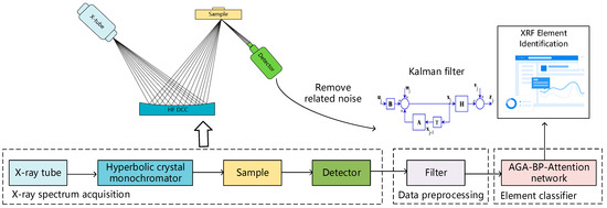
Figure 1.
The X-ray Fluorescence (XRF) spectroscopy system and element identification framework.
STEP 1: The first step is the generation of the X-ray fluorescence spectroscopy data. The system primarily includes an X-ray tube, a hyperbolic crystal, the sample, and a detector.
The X-ray tube, essentially a high-voltage diode, consists of an electron-emitting cathode and an electron-collecting anode housed in a vacuum-sealed tube. The cathode, typically a tungsten coil, emits a cloud of electrons when current is applied. These electrons, accelerated by the anode’s high voltage, interact with the target material to produce X-rays [17]. These X-rays are focused and monochromatized by a hyperbolic crystal [18]. Incident X-rays parallel to the crystal’s cylindrical surface satisfy the Bragg condition. Utilizing the symmetry of the Rowland focusing circle, each diffracted ray converges onto a parallel line on the circle’s opposite side, boosting the crystal’s diffraction intensity. A two-dimensional curvature crystal technique adapts the diffraction from a point light source into a focused spot on the detector window, allowing for a larger crystal without being limited by the detector’s window area.
The resulting fluorescence X-rays are focused onto the detector. The detector transforms these X-ray fluorescence photons into distinct counts and shapes of electric pulses, representing the energy and intensity of the X-ray fluorescence, subsequently generating the X-ray fluorescence spectrum [19]. By measuring the fluorescence spectrum, we can obtain information about the elements in the sample [20]. Each element has a unique inner energy level structure, making the energy level difference and wavelength of the fluorescence emission characteristic of the element. By analyzing the fluorescence spectrum, we can determine the elements in the sample.
STEP 2: The second step is data preprocessing. At this point, a Kalman filter is applied to the spectral data. The Kalman filter is a recursive linear optimization algorithm that can provide the best estimate of the system state at each step, even in the presence of noisy measurements and process uncertainty. In this context, the “system state” is the elemental composition of the sample, and the “measurements” are the spectral data recorded by the SDD detector. The Kalman filter, considering the statistical characteristics of measurement and process noise, as well as system dynamics, can offer a more accurate and stable estimate of the elemental composition of the sample. This preprocessing step allows for more accurate and stable data to be inputted into the neural network, enhancing its feature extraction and predictive capabilities.
STEP 3: Finally, spectral analysis is conducted using the feature extraction and predictive abilities of a BP-Attention neural network algorithm. This algorithm interprets the spectrum and identifies the types of elements present in the sample. The key advantage of the BP-Attention network lies in its powerful non-linear fitting capability and adaptability to model and predict complex patterns in the spectral data. Furthermore, the attention mechanism within this network emphasizes the importance of certain spectral features, greatly enhancing the accuracy of element identification.
4. X-ray Spectrum Data Acquisition and Preprocessing
The samples of multiple air pollutant filters were probed with three energy levels (low, medium, and high) of a high-sensitivity X-ray fluorescence spectrometer, resulting in raw spectrum data, as shown in Figure 2. The spectral data were divided into the smallest units of each 10 eV energy segment, and the average intensity count and variation rate of the same segment on three energy levels were noted.
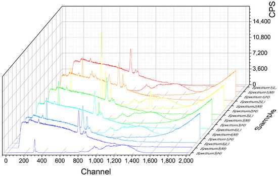
Figure 2.
The raw X-ray fluorescence spectrum.
However, like many other analytical techniques, XRF spectroscopy can be affected by noise, which can distort the original signal and potentially lead to inaccurate results. Statistical noise, electronic noise, background noise, and environmental noise are the four main types of noise in XRF spectroscopy. The Kalman filter algorithm, as an excellent denoising algorithm, is widely used in signal noise suppression [21,22]. To mitigate the interference caused by these noise elements on the network model recognition, we employed the Kalman filter to process the X-ray fluorescence spectrum.
The Kalman filter is a recursive estimation algorithm that provides an efficient computational solution to the least-squares method. It is used to estimate the state of a linear dynamic system under the presence of random noise. The algorithm works in a two-step process:
Firstly, the Kalman filter primarily consists of two steps: the prediction step and the update step.
The prediction step uses the system’s dynamic model to transition the state from time t to time t + 1. Specifically, if you have a state vector and a control vector , it can predict the next state using the following equation:
where is the state transition matrix and is the control input matrix.
The prediction step also predicts the covariance of the state :
where is the process noise covariance matrix and is the transpose of .
The update step updates the prediction upon receiving new observation data. If you have an observation vector , you can compute the updated state and covariance using the following equations:
where is the observation model, is the observation noise covariance matrix, and is the Kalman gain. Note that these equations are derived assuming that all errors (including process noise and observation noise) are Gaussian distributed.
As depicted in Figure 3, the spectral data, after being filtered through the Kalman filter, have a significant amount of noise removed. While preserving the original trend of the curve, the process makes the curve smoother. The elimination of noise fluctuations substantially reduces the variations in the dataset’s gradient, thereby lowering the probability of subsequent neural network recognition failure.
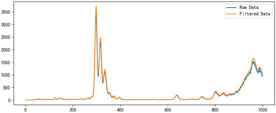
Figure 3.
Filtered data after preprocessing by Kalman filter.
5. AGA-BP-Attention Neural Network
Considering the inherent characteristics of X-ray spectra, where each distinct element may manifest only within specific channels and the relevance of each element is intricately tied to the peak count-per-second (CPS) and gradient within its respective channel, we postulate that the importance of individual data points within our dataset varies in terms of elemental identification.
As shown in (8), X represents the data information contained in the data set, where is the channel count. , , and are the number of photons received by the instrument at high, medium, and low energy grades, respectively. , , and are the photon count gradient, i.e., the difference between the number of photons in this channel and the next channel. is the element determination label.
To address this, we have strategically incorporated an attention mechanism into the conventional Backpropagation (BP) neural network, which enables the model to prioritize and concentrate on the more informative aspects of the data. Furthermore, in an effort to enhance the efficiency of our model, we have utilized a genetic algorithm to optimize the initial weight parameters of the neural network, thereby effectively accelerating the convergence rate.
5.1. Model Optimization by the Adaptive Genetic Algorithm
Genetic algorithms are commonly used to improve the global optimization ability of algorithm models [23,24]. Genetic algorithms are optimization techniques inspired by the process of natural selection. They are used to find solutions to optimization and search problems by iteratively selecting, combining, and mutating candidate solutions based on their performance, as measured by a fitness function. In the AGA-BP-Attention network, the GA would help to optimize the BP network and Attention model’s parameters for better performance.
First, the related design and definition of formulas in genetic algorithms will be explained.
Fitness assessment constitutes the core step in the optimization of the neural network. The fitness function can be used to evaluate the quality of the optimized neural network parameters.
As shown in Equation (9), the reciprocal of the neural network’s loss function is utilized as the fitness function. In this context, y denotes the labels, and x represents the output of the neural network. The model’s loss is obtained by calculating the squared difference between them. Obviously, the smaller the loss value predicted by the neural network, the greater the fitness value, and the better the optimization effect of the genetic algorithm.
Once the algorithm obtains some initial neural network parameters, the algorithm can treat them as parent solutions for optimizing the neural network and calculate their fitness. The selected parent individuals undergo crossover and mutation operations to generate new offspring (i.e., obtain new solutions).
Equation (10) defines the probability calculation formulas for chromosome crossover. Here, and denote predefined constants that determine the range within which the crossover probability can adapt. is the adaptive crossover probability for an individual based on its fitness. is the larger fitness value between the two individuals to be crossed. is the maximum fitness value in the current population. is the average fitness value of the current population.
Similarly, Equation (11) defines the probability calculation formulas for chromosome mutation. and denote predefined constants that determine the range within which the mutation probability can adapt. is the fitness value of the individual to be mutated currently. The other parameters have the same meaning as the above equation.
Figure 4 demonstrates the crossover and mutation processing in the GA. In crossover processing, between two copies randomly selected by , a crossover point is randomly selected, and then the chromosome parts before and after the crossover point are crossed and swapped between chromosomes, thus producing new offspring. In mutation processing, a certain gene on the string is changed according to each unit in the solution, based on probability . It should be noted that each number in the solution denotes the parameters of the neural network.
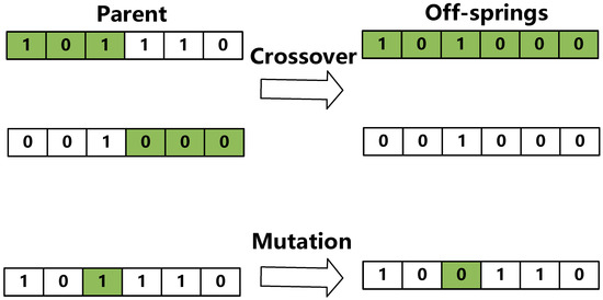
Figure 4.
Crossover and mutation processing in the GA.
The flowchart depicted in Figure 5 outlines an innovative approach where the initial weights and biases of the Backpropagation (BP) neural network are encoded as the genetic makeup of individuals within a Genetic Algorithm (GA) population. Each individual’s genetic structure mirrors the architecture of the BP network, with the length of the genetic sequence directly corresponding to the total number of weights and biases present.
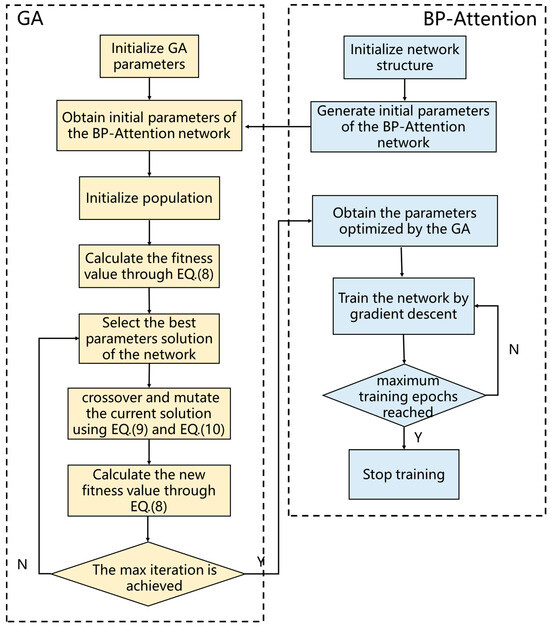
Figure 5.
Flowchart of the adaptive genetic algorithm.
The population consists of a set of individuals, each representing a neural network. The goal of initializing the population is to create a diverse set of initial solutions, providing ample space for the subsequent evolutionary process to search for the optimal solution. Each chromosome (individual) is composed of four parts: hidden layer weights, hidden layer biases, output layer weights, and output layer biases. The chromosomes are encoded in a serial concatenation by row, following the order of weights, biases, weights, and biases. A set number of these chromosomes constitute the initial population for genetic algorithm training.
Following selection, the crossover operation is applied, where pairs of selected individuals exchange segments of their genetic code, which here represents the neural network parameters. This genetic recombination fosters diversity within the population and allows for the exploration of new regions in the solution space, potentially leading to better performance.
Mutation plays a critical role by introducing random changes to individual genes—specific weights or biases in the context of the neural network. The purpose of this randomness is to prevent the evolutionary process from becoming stagnant and to help escape local optima by providing innovative solutions for evaluation.
The GA’s role is to repeatedly refine these initial parameters through its selection, crossover, and mutation processes until the network achieves a predefined threshold of recognition accuracy. Once this threshold is reached, indicating that the GA has sufficiently optimized the initial parameters, it halts any further updates.
With the cessation of the GA’s optimization, the neural network transitions to gradient descent training. This phase involves fine-tuning the optimized parameters by making small, iterative adjustments in the direction that minimizes the error. This training phase continues until the network has completed the maximum allotted number of training epochs, ensuring that the network’s learning is as thorough as possible.
5.2. BP-Attention Neural Network
The concept of attention in neural networks, originating from the field of human cognitive psychology, is inspired by the observation that when humans process visual scenes, they do not consider all information uniformly. Instead, they dynamically focus their attention on different parts of the scene based on their relevance. In the context of neural networks, the attention mechanism was first introduced in the field of natural language processing (NLP) with the transformer model by [25].
The BP-Attention neural network combines the BP network with the attention mechanism. In this model, the attention mechanism is used to assign different weights or “attention” to different parts of the input data. These weighted data are then fed into the BP neural network.
The elements being tested are divided into five categories: Fe, Ni, Cu, Mn, and other interference peaks. As shown in Figure 6, a classifier that combines a dot-product attention mechanism with a three-layer backpropagation (BP) neural network is constructed using the PyTorch framework based on Python. Initially, data are input into the attention heads; each neuron in the input layer of the BP neural network corresponds to each input feature value, and the five neurons in the output layer correspond to the five types of elements. The number and layers of neurons in the hidden layer are key parameters that affect the training effect and computation time. The number of neurons in the hidden layer is initially determined to be ten according to the empirical formula, and then the training effects when the number of neurons is eight, nine, eleven, and twelve are examined. The results show that the error index of the neural network is the smallest when the number of neurons is ten.
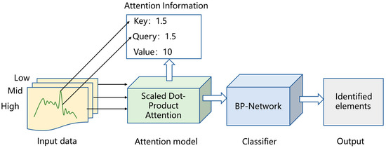
Figure 6.
BP-Attention neural network structure.
Scaled dot-product attention is a type of attention mechanism that is used in many state-of-the-art models like Transformers for tasks such as machine translation and text summarization [26,27]. The main idea behind the attention mechanism is to focus on the most relevant parts of the input when processing data. In this study, we aim to employ the dot-product attention mechanism to enable the network to learn the significance of different energy levels and noise for element recognition. As shown in Figure 7, the scaled dot-product attention mechanism works in the following steps:
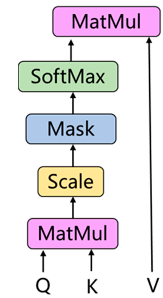
Figure 7.
Scaled dot-product attention structure.
Input: The attention function takes in three inputs—Queries (Q), Keys (K), and Values (V). These are usually matrices where each row represents a specific instance. The Queries, Keys, and Values are created by transforming the input data (e.g., word embeddings). In the context of the Transformer model, these transformations are performed by learned linear projections.
Dot Product of Q and K: The attention score is computed by taking the dot product between the Query and the Key. This score reflects the relevance of the respective Key–Value pair to the Query.
Scaling: The dot product tends to increase with the dimensionality of the Query and Key vectors. To control this, the dot product is scaled down by a factor of the square root of the dimension of the key vectors.
The scaling factor is , where is the dimension of the keys.
Apply Softmax: The Softmax function is applied to the scaled dot-product of the Query and Key to obtain a probability distribution. This gives the weights, which sum up to 1 and are used as the coefficients for the weighted sum of the Values.
Multiply by V: After the Softmax normalization is performed on the keys to derive their weights, these weights are used to take a weighted sum of the Values. The Softmax score determines the amount of attention paid to each Value—a high Softmax score means the value is considered important in the context of the given query.
The mathematical expression for scaled dot-product attention structure can be expressed as:
The output is a weighted sum of the values, based on the attention scores (i.e., the Softmax scores).
6. Results
In this section, we present simulation results that validate the effectiveness of the proposed approach. The experiments were performed on a system equipped with an Intel i7 13700k CPU, an RTX4080 GPU, and 32GB of RAM. PyTorch version 1.12.0 was employed for conducting the experiments. We validated our approach from two aspects: the optimization of neural network parameters by the genetic algorithm, and the accuracy of the neural network in spectral recognition.
Figure 8 demonstrates the fitness iterative process of the genetic algorithm. During the initial stage of the iteration, from generation 0 to 30, the fitness of the algorithm was 18.8. After iterating from generation 30 to 32, the fitness improved to 19.2 through methods such as selection, crossover, and mutation. By the time it iterated to the 40th generation, the fitness reached 19.3. The fitness was effectively improved, and convergence was achieved. In this paper, the fitness is set up to be inversely proportional to the loss value of the neural network. Therefore, with the increase in fitness, we can infer that the genetic algorithm has effectively optimized the initial parameters of the neural network, reducing the neural network’s loss value.
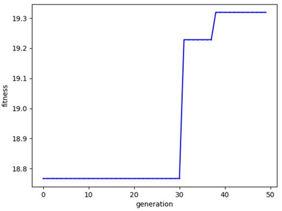
Figure 8.
The iterative process of the genetic algorithm.
Subsequently, we compared the impact of the genetic algorithm on the convergence of neural network training. Figure 9 illustrates the convergence process of the loss value in the BP-Attention network with and without the genetic algorithm. Compared to the original BP-Attention network, the loss value after optimization by the genetic algorithm shows a certain degree of reduction. Specifically, under the initial parameters, the loss value of the GA-BP-Attention network is as low as 9, while that of the BP-Attention network is as high as 23, marking a 60% reduction in the loss value. Furthermore, the convergence speed of GA-BP-Attention is faster than that of BP-Attention. A lower loss value also implies that the classification effect of the network model will be better.
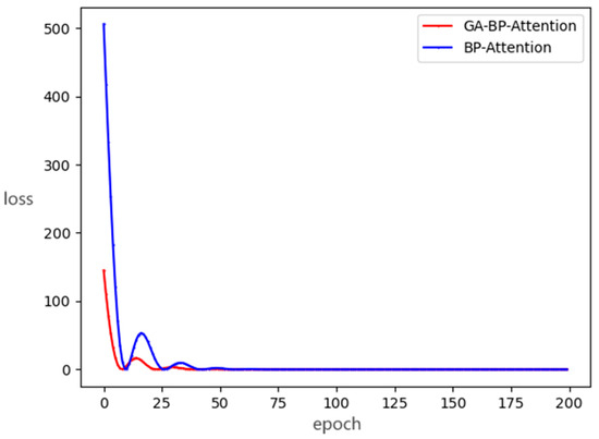
Figure 9.
The loss comparison between GA-BP-Attention and BP-Attention.
Figure 10 depicts the recognition accuracy of AGA-BP-Attention, where the blue curve represents the predicted values and the red curve represents the actual values. It can be observed that, in the process of chemical element recognition in air pollutant samples, the predicted curve exhibits a good fit and high recognition accuracy. The recognition accuracy reaches as high as 95.75%. This can, to a certain extent, suppress the impact of background noise on spectral element recognition.
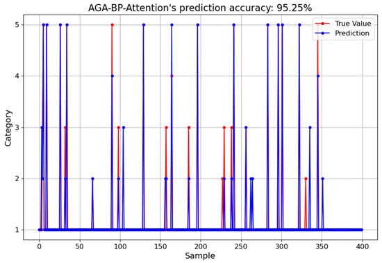
Figure 10.
The prediction accuracy of AGA-BP-Attention.
Figure 11 presents the recognition accuracy of the AGA-BP algorithm, a comparative baseline without the attention module. The blue curve illustrates the predicted values, whereas the red curve displays the actual values. In the context of chemical element recognition within air pollutant samples, the AGA-BP algorithm demonstrates a decent fit and a reasonable level of recognition accuracy, achieving an accuracy peak of 79.5%.
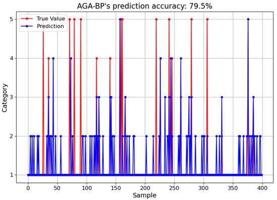
Figure 11.
The prediction accuracy of AGA-BP.
However, when juxtaposed with the AGA-BP-Attention algorithm, the performance of AGA-BP appears less robust. The absence of the attention module in the AGA-BP algorithm leads to a noticeable decline in recognition accuracy. The impact of background noise is also more pronounced, suggesting a reduced capability to effectively handle such disturbances. This comparative analysis clearly highlights the superior performance of the AGA-BP-Attention algorithm, demonstrating the critical role of the attention module in enhancing recognition accuracy and managing background noise.
7. Conclusions
To address the challenges of high nonlinearity and noise in X-ray fluorescence (XRF) spectral recognition, which complicate spectral identification, this paper adopts a deep-learning-based approach to overcome these obstacles, proposing the AGA-BP-Attention method. This method utilizes an adaptive genetic algorithm to optimize the initial parameters of the network module. Moreover, by integrating an Attention mechanism, the model’s focus is directed towards the recognition of effective spectral components. It is proved through experiments that the AGA-BP-Attention model leverages the robust feature extraction capabilities of the neural network and the power of the attention mechanism, effectively recognizing the elemental signatures in air pollutant samples.
Author Contributions
Conceptualization, Z.C. and Q.Z.; methodology, Z.C.; software, Y.L.; validation, Y.L. and R.G.; formal analysis, R.G.; investigation, Y.T.; resources, Y.T.; data curation, L.R.; writing—original draft preparation, L.R.; writing—review and editing, M.S.; visualization, M.S.; supervision, Q.Z. and X.X.; project administration, X.X.; funding acquisition, Q.Z. All authors have read and agreed to the published version of the manuscript.
Funding
This work is supported by the National Major Scientific Instruments and Equipment Development Project of the National Natural Science Foundation of China (No. 62127816).
Data Availability Statement
The data are unavailable due to privacy or ethical restrictions.
Conflicts of Interest
The authors declare no conflicts of interest.
References
- Kampa, M.; Castanas, E. Human health effects of air pollution. Environ. Pollut. 2008, 151, 362–367. [Google Scholar] [CrossRef] [PubMed]
- Shackley, M.S. An introduction to X-ray fluorescence (XRF) analysis in archaeology. In X-ray Fluorescence Spectrometry (XRF) in Geoarchaeology; Springer: New York, NY, USA, 2011; pp. 7–44. [Google Scholar]
- De Jonge, M.D.; Vogt, S. Hard X-ray fluorescence tomography—An emerging tool for structural visualization. Curr. Opin. Struct. Biol. 2010, 20, 606–614. [Google Scholar] [CrossRef] [PubMed]
- Dos Anjos, M.J.; Lopes, R.T.D.; de Jesus, E.F.O.; Assis, J.; Cesareo, R.; Barradas, C. Quantitative analysis of metals in soil using X-ray fluorescence. Spectrochim. Acta Part B Spectrosc. 2000, 55, 1189–1194. [Google Scholar] [CrossRef]
- Haga, A.; Senda, S.; Sakai, Y.; Mizuta, Y.; Kita, S.; Okuyama, F. A miniature X-ray tube. Appl. Phys. Lett. 2004, 84, 2208–2210. [Google Scholar] [CrossRef]
- Rousseau, R.M. The quest for a fundamental algorithm in X-ray fluorescence analysis and calibration. Open Spectrosc. J. 2009, 9, 3. [Google Scholar] [CrossRef][Green Version]
- Kamilaris, A.; Prenafeta-Boldú, F.X. Deep learning in agriculture: A survey. Comput. Electron. Agric. 2018, 147, 70–90. [Google Scholar] [CrossRef]
- Jun, C.; Hongchang, F.; Zhe, L.; Zhao, Z. Soft measurement of reforming catalyst carbon accumulation in DCS using neural network. Petrochem. Autom. 2015, 51, 29–32. [Google Scholar] [CrossRef]
- Schimidt, F.; Cornejo-Ponce, L.; Bueno, M.I.M.S.; Poppi, R.J. Determination of some rare earth elements by EDXRF and artificial neural networks. X-ray Spectrom. Int. J. 2003, 32, 423–427. [Google Scholar] [CrossRef]
- Li, F.; Ge, L.Q.; Zhang, Q.X.; Gu, Y.; Wan, Z.X.; Li, W.Y. Application of improved M-P neural network in energy dispersive X-fluorescence analysis for the determination of lead and zinc ores. Spectrosc. Spectr. Anal. 2012, 32, 1410–1412. [Google Scholar]
- Chung, F.H. Unified Theory for Decoding the Signals from X-ray Florescence and X-ray Diffraction of Mixtures. Appl. Spectrosc. 2017, 71, 1060–1068. [Google Scholar] [CrossRef] [PubMed]
- Ye, S.B.; Xu, L.; Li, Y.K.; Liu, J.G.; Liu, W.Q. Study on Recognition of Cooking Oil Fume by Fourier Transform Infrared Spectroscopy Based on Artificial Neural Network. Spectrosc. Spectr. Anal. 2017, 37, 749–754. [Google Scholar]
- Yan, S.; Huang, J.-J.; Verinaz-Jadan, H.; Daly, N.; Higgitt, C.; Dragotti, P.L. A Fast Automatic Method for Deconvoluting Macro X-ray Fluorescence Data Collected from Easel Paintings. IEEE Trans. Comput. Imaging 2023, 9, 649–664. [Google Scholar] [CrossRef]
- Ahmed, M.F.; Yasar, S.; Cho, S.H. A Monte Carlo Model of a Benchtop X-ray Fluorescence Computed Tomography System and Its Application to Validate a Deconvolution-Based X-ray Fluorescence Signal Extraction Method. IEEE Trans. Med. Imaging 2018, 37, 2483–2492. [Google Scholar] [CrossRef] [PubMed]
- Fiske, L.D.; Katsaggelos, A.K.; Aalders, M.C.G.; Alfeld, M.; Walton, M.; Cossairt, O. A Data Fusion Method for the Delayering of X-ray Fluorescence Images of Painted Works of Art. In Proceedings of the 2021 IEEE International Conference on Image Processing (ICIP), Anchorage, AK, USA, 19–22 September 2021; pp. 3458–3462. [Google Scholar] [CrossRef]
- Rahman, A.; Shahriar, S.; Timms, G.; Lindley, C.; Davie, A.B.; Biggins, D.; Hellicar, A.; Sennersten, C.; Smith, G.; Coombe, M. A machine learning approach to find association between imaging features and XRF signatures of rocks in underground mines. In Proceedings of the 2015 IEEE SENSORS, Busan, Republic of Korea, 1–4 November 2015; pp. 1–4. [Google Scholar] [CrossRef]
- Longoni, A.; Fiorini, C.; Guazzoni, C.; Buzzetti, S.; Bellini, M.; Struder, L.; Lechner, P.; Bjeoumikhov, A.; Kemmer, J. XRF spectrometers based on monolithic arrays of silicon drift detectors: Elemental mapping analyses and advanced detector structures. IEEE Trans. Nucl. Sci. 2006, 53, 641–647. [Google Scholar] [CrossRef]
- Chang, W.Z.; Forster, E. X-ray diffractive optics of curved crystals: Focusing properties on a diffraction-limited basis. J. Opt. Soc. Am. A 1997, 14, 1647–1653. [Google Scholar] [CrossRef]
- Amoyal, G.; Menesguen, Y.; Schoepff, V.; Carrel, F.; Michel, M.; Angelique, J.-C.; de Lanaute, N.B. Evaluation of Timepix3 Si and CdTe Hybrid-Pixel Detectors’ Spectrometric Performances on X- and Gamma-Rays. IEEE Trans. Nucl. Sci. 2021, 68, 229–235. [Google Scholar] [CrossRef]
- Chen, X.; Chen, Q.; Shi, Q. X-ray fluorescence spectroscopy analysis method and its application. Environ. Technol. 2015, 33, 25–27+31. [Google Scholar]
- Tan, F.; Bao, C. Kronecker Product Based Linear Prediction Kalman Filter for Dereverberation and Noise Reduction. In Proceedings of the 2021 IEEE International Conference on Signal Processing, Communications and Computing (ICSPCC), Xi’an, China, 17–19 August 2021; pp. 1–5. [Google Scholar] [CrossRef]
- Hesar, H.D.; Mohebbi, M. An Adaptive Kalman Filter Bank for ECG Denoising. IEEE J. Biomed. Health Inform. 2021, 25, 13–21. [Google Scholar] [CrossRef] [PubMed]
- Sabbah, T. Enhanced Genetic Algorithm for Optimized Classification. In Proceedings of the 2020 International Conference on Promising Electronic Technologies (ICPET), Jerusalem, Palestine, 16–17 December 2020; pp. 161–166. [Google Scholar] [CrossRef]
- Li, K.; Jia, L.; Shi, X. An Efficient Hybridized Genetic Algorithm. In Proceedings of the 2018 IEEE International Conference of Safety Produce Informatization (IICSPI), Chongqing, China, 10–12 December 2018; pp. 118–121. [Google Scholar] [CrossRef]
- Vaswani, A.; Shazeer, N.; Parmar, N.; Uszkoreit, J.; Jones, L.; Gomez, A.N.; Kaiser, Ł.; Polosukhin, I. Attention is all you need. In Proceedings of the 31st International Conference on Neural Information Processing Systems (NIPS’17), Long Beach, CA, USA, 4–9 December 2017; Curran Associates Inc.: Red Hook, NY, USA, 2017; pp. 6000–6010. [Google Scholar]
- Leelaluk, S.; Minematsu, T.; Taniguchi, Y.; Okubo, F.; Yamashita, T.; Shimada, A. Scaled-Dot Product Attention for Early Detection of At-risk Students. In Proceedings of the 2022 IEEE International Conference on Teaching, Assessment and Learning for Engineering (TALE), Hung Hom, Hong Kong, 14 June 2022; pp. 316–322. [Google Scholar] [CrossRef]
- Zhang, C.; Wang, D.; Jia, J.; Wang, L.; Chen, K.; Guan, L.; Liu, Z.; Zhang, Z.; Chen, X.; Zhang, M. Potential failure cause identification for optical networks using deep learning with an attention mechanism. J. Opt. Commun. Netw. 2022, 14, A122–A133. [Google Scholar] [CrossRef]


Disclaimer/Publisher’s Note: The statements, opinions and data contained in all publications are solely those of the individual author(s) and contributor(s) and not of MDPI and/or the editor(s). MDPI and/or the editor(s) disclaim responsibility for any injury to people or property resulting from any ideas, methods, instructions or products referred to in the content. |
© 2024 by the authors. Licensee MDPI, Basel, Switzerland. This article is an open access article distributed under the terms and conditions of the Creative Commons Attribution (CC BY) license (https://creativecommons.org/licenses/by/4.0/).