MixMobileNet: A Mixed Mobile Network for Edge Vision Applications

Abstract

Currently, vision transformers (ViTs) have rivaled comparable performance to convolutional neural networks (CNNs). However, the computational demands of the transformers’ self-attention mechanism pose challenges for their application on edge devices. Therefore, in this study, we propose a lightweight transformer-based network model called MixMobileNet. Similar to the ResNet block, this model only comprises a MixMobile block (MMb), which combines the efficient local inductive bias with the explicit modeling features of a transformer to achieve the fusion of the local–global feature interactions. For local, we propose the local-feature aggregation encoder (LFAE), which incorporates a PC2P (Partial-Conv→PWconv→PWconv) inverted bottleneck structure for residual connectivity. In particular, the kernel and channel scale are adaptive, reducing feature redundancy in adjacent layers and efficiently representing parameters. For global, we propose the global-feature aggregation encoder (GFAE), which employs a pooling strategy and computes the covariance matrix between channels instead of the spatial dimensions, changing the computational complexity from quadratic to linear, and this accelerates the inference of the model. We perform extensive image classification, object detection, and segmentation experiments to validate model performance. Our MixMobileNet-XXS/XS/S achieves 70.6%/75.1%/78.8% top-1 accuracy with 1.5 M/3.2 M/7.3 M parameters and 0.2 G/0.5 G/1.2 G FLOPs on ImageNet-1K, outperforming MobileViT-XXS/XS/S with an improvement of +1.6%↑/+0.4%↑/+0.4%↑ with −38.8%↓/−51.5%↓/−39.8%↓ reduction in FLOPs. In addition, the MixMobileNet-S assembly of SSDLite and DeepLabv3 achieves an accuracy of 28.5 mAP/79.5 mIoU at COCO2017/VOC2012 with lower computation, demonstrating the competitive performance of our lightweight model.

1. Introduction

In recent years, Google successfully applied a transformer (used in the field of natural language processing (NLP)) to computer vision (CV) and surpassed CNN-based state-of-the-art (SOTA) models at that time (ResNet152×4 [1]). This has triggered research workers to pay further attention to transformers, and subsequent work on vision transformers, such as DeiT [2], SwinT [3], PVT [4], DETR [5], Segformer [6], etc., has been proposed one after another. However, it is important to note that training ViTs models often requires the use of GPU clusters (e.g., TPUv3, Nvidia A100) and large-scale training datasets (e.g., ImageNet-21K [7], JFT-300M), which inevitably consumes significant computational resources.

With the increasing integration of artificial intelligence technology in daily production and life fields, such as autonomous driving, mixed reality, 6-DoF robot grasping, and other edge applications, the demand for feature extraction networks requires fast devices with lightweight inference. Marginalizing the transformer-based model poses a challenge due to its high computation requirements; nevertheless, it serves as inspiration for our work. Previously, mobile networks like MobileNet [8,9,10], ShuffleNet [11], EfficientNet, [12] and GhostNet [13] have been dominant for lightweight vision tasks. Despite having fewer parameters and FLOPs, these models find it difficult to capture global perception implicitly, creating challenges for lightweight CNNs. This, in turn, leads to low parameterization efficiency and weak inference performance. Through researching models such as Swin-T [3], PVT-v1 [4], DeiT [2], and T2T-ViT [14], researchers have discovered that the cascaded self-attention mechanism in ViT can capture long-range feature dependencies, effectively compensating for the explicit modeling difficulties and lack of input flexibility in CNNs. However, ViT-pure models lack convolution-like local inductive biases, and their performance is sensitive to hyper-parameters. To address the limitations of current networks, researchers have experimented with combining CNNs and ViTs, including CeiT [15], CCT [16], and PVT-v2 [17]. This approach has proved successful in boosting the model’s performance on baseline tasks. Nevertheless, it can lead to a decrease in inference efficiency due to the operator of ViTs, self-attention, which has a quadratic relationship with input size, ultimately impacting the model’s inference speed. Therefore, it does not ensure a balance between the speed and accuracy of resource-limited devices.

Our MixMobileNet achieves competitive performance compared to lightweight convolutional neural networks and recent hybrid architecture networks. We strike a balance between parameters, FLOPs, and performance in our work.

Recently, a lightweight hybrid architecture model named MobileViTv1 [18] has been designed specifically for mobile devices. It combines the strengths of MobileNetv2 (MV2) [9] and ViT [19], achieving SOTA performance in various mobile vision tasks. The model’s inference speed is slow, even with only 5.6 M parameters and 2.1 G MAdds, due to the spatial self-attention mechanism. The visualized research indicates that the MV2 block [9] results in feature duplication and redundant kernel parameters within the model [20]. Moreover, lightweight inference is hindered by the limited ability to compute global interactions in the spatial dimension due to input size constraints. Similarly, EdgeNeXt [21] combines depth-wise separable convolution and transposed attention mechanisms to introduce a split depth-wise transpose attention that enhances resource utilization. However, the structural design of this model is dependent on intricate submodules, such as Res2Net [22], ConvNeXt [23], and XCA [24]. Moreover, other related works incorporate EdgeViTs [25], the MobileFormer [26], EfficientFormer [27], and FasterViT [28]. A significant issue is that these architectures differ from ResNet in terms of simplicity and efficiency, which relies on complex structures and neural architecture search techniques [29,30]. To enhance the model’s performance, they rely on neural architecture search techniques or model pruning means. Therefore, the objective of this study is to create lightweight networks for devices with limited resources (e.g., Nvidia-AGX) through a fusion of CNNs’ and ViTs’ advantages. The objective is to enhance the plug-and-play functionality and ease of module integration.

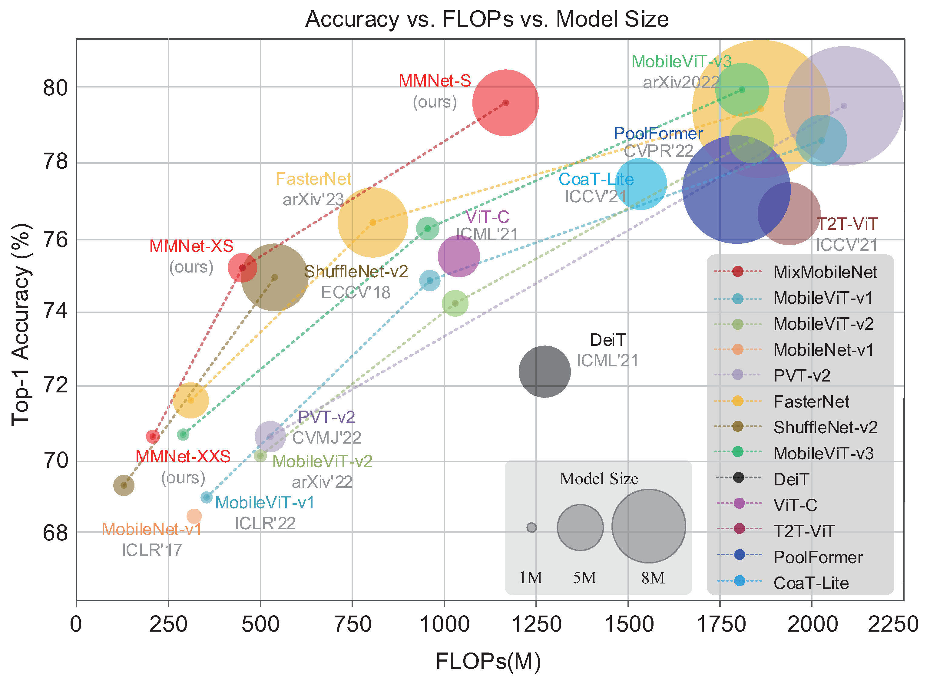
We propose an efficient and lightweight visual architecture named MixMobileNet. The model’s body employs solely MixMobile block (MMb)as its primary component and is supported by two interrelated feature extraction blocks: the local-feature aggregation encoder (LFAE) and the global-feature aggregation encoder (GFAE). These blocks are utilized for constructing information encodings that combine the advantages of convolutional neural networks’ efficient local-inductive bias with transformers’ dynamic long-range modeling capabilities. This integration leads to enhanced performance effectiveness, as depicted in Figure 1.

Our contributions are as follows:

• This work proposes a lightweight feature extraction network called MixMobileNet. It combines the efficient local inductive bias of convolutional neural networks and the pixel-level long-range global modeling capability of transformers. By using an effective feature pyramid structure, it aggregates token information in multiple stages to generate high-density predictive capabilities.
• We propose a plug-and-play MMb as the model’s basic block. In the overall design, we introduce two layers of encoders: LFAE and GFAE, which are used for local and global feature extraction and block-level local-global feature fusion, respectively.
• Without introducing complex structures, our models have achieved competitive results on several benchmark tests. For example, our MixMobileNet-XXS/XS/S achieve 70.6%/75.1%/78.8% top-1 accuracy on the ImageNet-1K dataset [7]. Additionally, when combined with SSDLite [9]/DeepLabv3 [31], MixMobileNet-S achieves 28.5 mAP/79.5 mIoU with 8.3 M/6.9 M parameters, resulting in a +2.8%↑/+0.5%↑ improvement over the recent MobileViT-S [18].

The remaining content is organized as follows: Section 2 details the relevant research advances in lightweight CNNs and ViTs; Section 3 introduces the general design and detailed description of MixMobileNet; in Section 4, we conduct a series of experiments and report the final results; and Section 5 summarizes our work.

2. Related Work

CNN-based. In recent years, convolutional neural networks and residual connection structures, such as ResNet [1], RegNet [30], and DenseNet [32], have significantly improved the accuracy of image classification. However, for convolutional neural network models with parameters reaching hundreds of M and computational requirements reaching tens of G FLOPs, both training and inference rely heavily on large-scale GPU clusters. As a result, it becomes challenging to apply these models to low-powered edge devices. Therefore, starting with SqueezeNet [33], Iandola et al. [33] begin to explore the efficiency of deep neural networks in resource-constrained situations. Subsequently, some lightweight CNN-based models such as MobileNet series [8,9,10], EfficientNet Lite series [12], ShuffleNet series [11], and Huawei’s GhostNet [13] have been proposed, and they have shown significant improvements in both speed and accuracy. Among them, Howard et al. [8] propose the depth-wise separable convolution, which reduces the computational complexity of traditional convolution by nearly an order of magnitude. This innovation makes MobileNetv1 [8] the first successful network in the field of lightweight models. Tan et al. [12] propose a new scaling method called compound model scaling, which uniformly scales all dimensions of depth/width/resolution using a simple yet highly effective compound coefficient to improve network performance. This research work is also the first to simultaneously investigate the impact of depth, width, and resolution on network performance. Ma et al. [11] propose point-wise group convolution and channel shuffle to reduce the computational complexity. These structures allow more feature map channels to encode more information for a given amount of computation, which greatly reduces the computational overhead while preserving the accuracy of the model. Lin et al. [23] design a purely convolutional architecture called ConvNeXt [23] by drawing inspiration from the ResNet [1] and Swin-T [3] networks and combining some design concepts of the ViT architecture. In the ConvNeXt [23] network, the authors innovatively change the number of blocks in each stage of ResNet50 [1] from [3, 4, 6, 3] to [3, 3, 9, 3], which improves the accuracy at the cost of increasing the computational complexity. Additionally, inspired by the design of the stem layer in ResNet [1], we modify the $7\times 7$ convolution with a stride of 2 to a $4\times 4$ convolution with a stride of 4. This modification further improves the accuracy of the model. The ConvNeXt [23] network architecture design has great significance to many later network designs. Recently, Chen et al. [34] proposed a novel partial convolution (PConv) that can extract spatial features more efficiently by cutting down redundant computation and memory access simultaneously. Furthermore, the point-wise convolution (PWconv) is appended to PConv to effectively integrate information from all channels. Their effective receptive field together on the input feature maps looks like a T-shaped convolution, which focuses more on the center position compared to a regular convolution uniformly processing a patch, allowing the network to be efficiently represented.

ViT-based. After the remarkable success of transformer encoding in the field of natural language processing (NLP), Dosovitskiy et al. [19] achieve comparable performance to convolutional architectures by serializing image sequences and feeding them into the transformer framework. Subsequently, its effectiveness has become increasingly prominent in tasks such as image classification, object detection, and autonomous driving, making it a widely adopted tool in computer vision (CV). However, transformers are typically computationally intensive. Specifically, they generate long sequences of feature tokens from high-resolution image inputs, which can increase the model’s inference workload and hinder its generalization to downstream tasks such as object detection and image segmentation. Additionally, achieving equivalent local inductive capabilities to CNNs with visual transformers requires training on large-scale datasets. Finally, the ViTs frameworks are sensitive to hyper-parameters and require patient and careful parameter tuning to achieve good convergence. To address the aforementioned issues, researchers have primarily focused on upgrading transformers from two perspectives: training settings and model architecture design. From the perspective of training settings, Touvron et al. have achieved impressive model performance in CaiT [35] and DeiT-III [2] by employing sophisticated data augmentation strategies and training techniques such as Mixup, CutMix, and Rand Augment. They have demonstrated outstanding results without relying on large proprietary datasets like JFT-300M. In DeiT [2], a distillation token and soft-distillation technique are used to compress the parameters of a powerful but large and difficult-to-train teacher model from 86 M to 5 M (DeiT-Tiny [2]). This compression leads to a tenfold improvement in inference speed. From the perspective of model architecture design, researchers have focused on two main directions: self-attention input resolution and attention mechanisms with low computational cost. PVT-v1 [4] emulates the feature map pyramid architecture found in CNNs by transforming the fixed 16× downsampling of the original ViTs into a multi-scale processing of the image. To address the issues of partial loss of spatial information at image edges and quadratic growth in computational complexity in ViT models, Liu et al. introduce a novel approach in Swin-T [3] and LightViT [36]. They incorporate a hierarchical feature map and shifted-window mechanisms to reduce the computational memory and complexity from quadratic to linear growth. As a result, these models exhibit superior performance compared to the original ViT [19] and DeiT models [2]. Deformable DETR [37] introduces the (multi-scale) deformable attention modules, which only attend to a small set of key sampling points around a reference point, regardless of the spatial size of the feature maps. This reduces computational complexity while maintaining a large receptive field. PVT [4], ResT [38], and CMT [39] use convolution to reduce the number of tokens corresponding to keys and values, thereby decreasing computational complexity. SOFT [40] uses the Gaussian kernel function to replace the softmax dot-product similarity and samples from the sequence by convolution or pooling to achieve a low-rank approximation to the original attention matrix.

Hybrid network. Compared to CNN-pure and ViT-pure models, the models that combine CNNs and ViTs not only have fewer parameters and faster inference but also demonstrate a significant improvement in network performance. Application deployment of ViT models poses significant challenges, especially on resource-constrained hardware like mobile devices. Recently, researchers focusing on mobile networks have paid attention to this problem. For instance, Apple’s MobileViTv1 [18] integrates the strengths of CNN into the transformer structure to address the training, transfer, and adaptation challenges inherent in transformer networks. Simultaneously, a core MobileViT block [18] is proposed to accelerate the inference and convergence speed of the network, making it more stable and efficient. Maaz et al. [21] propose a lightweight network called EdgeNeXt [21], which achieves a comprehensive balance between model size, parameters, and FLOPs. Furthermore, they introduce an efficient split depth-wise transpose attention (STDA) [21] encoder, enabling the effective fusion of local and global information representations. Pan et al. [25] propose a high-cost local–global–local (LGL) information exchange bottleneck based on the optimal integration of self-attention and convolution. Additionally, the LGL approach uses a sparse attention module to further mitigate the overhead of self-attention, achieving a better trade-off between accuracy and latency. Liu et al. [41] propose an EfficientViT block that includes a sandwich layout and cascaded group attention (CGA). This design aims to further reduce the inference latency caused by the extensive operations in the multi-head self-attention (MHSA) and the computational redundancy between attention heads. Li et al. [42] proposed a CNN-transformer hybrid architecture that utilizes the next hybrid strategy (NHS) strategy to stack the next convolution block (NCB) and next transformer block (NTB), enabling the fusion of local and global information and thus further enhancing the network’s modeling capability. Although most lightweight networks are designed with the goal of having fewer parameters, lower computational requirements, and low latency, they often require complex module designs, which greatly limit the model’s usability and reusability. Therefore, further research is needed to explore how to design a concise and efficient mobile model.

3. MixMobileNet

3.1. Overview

In order to design a lightweight vision transformer module that is simple, efficient, and suitable for deployment on mobile devices, we draw inspiration from the feature pyramid structure [3,43] in convolutional neural networks. By reducing the spatial resolution stage-by-stage [4,42,44] and expanding the channel dimensions simultaneously, the local and global features are continuously aggregated by two encoders LFAE and GFAE. At the local level, we integrate ResNet [1], ConvNeXt [23], and Partial-Conv [34] as the foundation and introduce a PC2P(Partial-Conv→PWconv→PWconv) inverted bottleneck structure to capture fine-grained information. At the global level, tokens generated from two-dimensional features are continuously aggregated to generate rich semantic expressions. The throughput of the module is accelerated by employing average pooling and channel attention strategies. By integrating local–global information, the extraction of features of different dimensions is enhanced, leading to improved network performance.

Our MixMobileNet is composed of four stages in structure, and each stage is stacked by MMb, which incorporates LFAE and GFAE, as shown in Figure 2. Specifically, the input image of size $\mathbf{X}\in {\mathbb{R}}^{H\times W\times 3}$ passed through the stem layer at the beginning of the network, which is composed of $4\times 4$ non-overlapping convolution and LayerNorm, resulting in $\mathbf{X}\in {\mathbb{R}}^{\frac{H}{4}\times \frac{W}{4}\times C_1}$ feature maps. Then, the output feature map is passed to the MMb, which is only composed of LFAE encoders. The second stage begins with a downsampling layer implemented using $2\times 2$ strided convolution that reduces the spatial sizes by half and increases the channels, resulting in $\mathbf{X}\in {\mathbb{R}}^{\frac{H}{8}\times \frac{W}{8}\times C_1}$ feature maps, and then passes through the MMb again. This layer consists of LFAE and GFAE to extract local and global features. The output feature maps are further passed to the third and fourth stages to generate $\mathbf{X}\in {\mathbb{R}}^{\frac{H}{16}\times \frac{W}{16}\times C_1}$ and $\mathbf{X}\in {\mathbb{R}}^{\frac{H}{32}\times \frac{W}{32}\times C_1}$ dimensional features, respectively, and then the global average pooling and fully connected layer are used to generate the prediction results. In addition, we set the positional encoding in the MMb of each stage, which can further improve the network expression performance. The configuration of the three variants of our model is shown in

Table 1. Configuration of the three MixMobileNet variants. Channels: number of channels per stage. #Depths: total number of blocks of global-feature aggregation encoders (GFAE) and local-feature aggregation encoders (LFAE) per stage. #LFAE: number of LFAE modules. #GFAE: number of GFAE modules. #Params: the number of parameters.

Model	Channels	#Depths	#LFAE	#GFAE	MAdds	#Params
MixMobileNet-XXS	[24, 48, 88, 168]	[2, 2, 6, 2]	[2, 1, 5, 1]	[0, 1, 1, 1]	0.2 G	1.5 M
MixMobileNet-XS	[32, 64, 100, 192]	[3, 3, 9, 3]	[3, 2, 4, 4]	[0, 1, 1, 1]	0.5 G	3.2 M
MixMobileNet-S	[48, 96, 160, 304]	[3, 3, 9, 3]	[3, 2, 4, 4]	[0, 1, 1, 1]	1.2 G	7.3 M

.

3.2. MixMobile Block

The self-attention mechanism in transformers helps the model explicitly establish global dependencies, thereby exhibiting superior performance compared to convolutional neural networks. When we study the work of Touvton et al. [2] and Simonyan et al. [45], we find some prominent problems: (a) for traditional ViTs, self-attention in the spatial dimension imposes a huge computational overhead due to the input resolution, and there is a huge challenge in deploying visual transformers on edge devices. (b) Although large kernel convolution adds more shape bias, they may overlook the capture of fine-grained features. Additionally, as the kernel size increases, the number of model parameters and FLOPs changes quadratically. To address the above problems, we propose a simple and efficient module called MMb. One of the GFAEs can effectively encode global information through the average pooling channel dimensionality reduction computation operation. This technique significantly reduces the computational overhead of the self-attention layer. The LFAE adopts a stage-by-stage adaptive kernel-size PConv [34] convolution. Smaller kernels are used at lower levels to extract local information, while larger kernels are used at deeper levels to capture more abstract global semantic features. This enables our model to obtain multi-scale features ranging from details to abstraction.

GFAE. To reduce redundancy between attention matrices, we employ average pooling on input feature tensors. In addition, we use cross-covariance across channels to generate attention feature maps, which linearly reduce the complexity of the original self-attention operation and effectively encode global information in an implicit manner. The details are as follows: given a feature map with input shape $\mathbf{X}(\in {\mathbb{R}}^{H\times W\times C})$, we compute query ($\mathbf{Q}$), key ($\mathbf{K}$), and value ($\mathbf{V}$) projections using three linear layers, yielding $\mathbf{Q}={\mathbf{W}}^Q\mathbf{X}(\in {\mathbb{R}}^{HW\times C})$, $\mathbf{K}={\mathbf{W}}^K\mathbf{X}(\in {\mathbb{R}}^{HW\times C})$, and $\mathbf{V}={\mathbf{W}}^V\mathbf{X}(\in {\mathbb{R}}^{HW\times C})$, where ${\mathbf{W}}^Q(\in {\mathbb{R}}^{C\times C})$, ${\mathbf{W}}^K(\in {\mathbb{R}}^{C\times C})$ and ${\mathbf{W}}^V(\in {\mathbb{R}}^{C\times C})$ are the projection weights of $\mathbf{Q}$, $\mathbf{K}$, and $\mathbf{V}$, respectively. Then, $L_2$ norm is applied to $\mathbf{Q}$ and $\mathbf{K}$ before computing the cross-covariance attention as it stabilizes the training, and we apply the dot-product across the channel dimensions between ${\mathbf{Q}}^T(\in {\mathbb{R}}^{C\times HW})$ and $\mathbf{K}(\in {\mathbb{R}}^{HW\times C})$ along the spatial dimension, i.e., $(\mathbf{C}\times \mathbf{H}\mathbf{W})·(\mathbf{H}\mathbf{W}\times \mathbf{C})$, producing a $(\mathbf{C}\times \mathbf{C})$ softmax-scaled attention score matrix. To obtain the final attention maps, we multiply the scores by $\mathbf{V}(\in {\mathbb{R}}^{HW\times C})$ and add them up. Finally, a residual connection is employed to ensure the flow of original fine-grained information from the previous stage, and the mathematical formulation of the above is as follows:

$$\widehat{\mathbf{X}}=Attention\left(\mathbf{Q},\mathbf{K},\mathbf{V}\right)+\mathbf{X}$$

(1)

$$S.t.,Attention\left(\mathbf{Q},\mathbf{K},\mathbf{V}\right)=\mathbf{V}·softmax\left(\parallel {\mathbf{Q}}^T{\parallel }_2·{\parallel \mathbf{K}\parallel }_2\right)$$

(2)

where $\mathbf{X}$ is the input and $\widehat{\mathbf{X}}$ is the output feature tensor. To achieve a smooth distribution of attention, we adopt the dropkey [46] regularization method in self-attention. By setting the key to a dropped object and verifying that it can penalize the high attention value portion, this approach alleviates the overfitting problem in self-attention. As the only nonlinear unit in self-attention, MLP provides high-latitude feature abstraction that can enrich the expressive power of the model even more. It uses two $1\times 1$ point-wise convolutional layers, layer normalization (LN) and Gaussian error linear unit (GELU) activations to generate nonlinear features. Specifically, channel upscaling is performed in the middle of the PW-conv layer at an adaptive scale. Our GFAE can be expressed as:

$${\mathbf{X}}_{Avg\_attn}=\varphi (pooling\left(\mathbf{X}\right)+Attention\left(pooling\left(\mathbf{X}\right)\right))$$

(3)

$${\mathbf{X}}_{MLP}=PWconv\left(\delta \left(PWconv\left(\sigma \left({\mathbf{X}}_{Avg\_attn}\right)\right)\right)\right)$$

(4)

$${\mathbf{X}}_{out}={\mathbf{X}}_{Avg\_attn}+{\mathbf{X}}_{MLP}$$

(5)

where $\mathbf{X}$ is the input, ${\mathbf{X}}_{out}$ is the output feature tensor, while ${\mathbf{X}}_{Avg\_attn}$ is the output feature tensor after the Avg-pooling layer and self-attention, $\varphi$ denotes the deconvolution operation (ConvTranspose2d), $\delta$ is the standard LN, and $\sigma$ is the GELU activation.

LFAE. We conducted an ablation study on the selection of the LAFE by comparing three methods: Figure 3a, a traditional convolution operation; Figure 3b, a depth-wise convolution; and Figure 3c, the method proposed in this study (Partial-Conv+SE). Furthermore, visual analysis (as shown in Figure 4) reveals that Rb [1] and MV2 [9] contain more salient $n\times n$ kernels in their intermediate feature parameters, such as the $n\times n$ fuzzy kernels with a large central value and smaller surrounding values. This redundancy leads to feature map repetition and unnecessary computation, which is detrimental to the design of lightweight models. From the results of the quantitative analysis, for the same number of parameters, the MAdds of our LFAE is 1.2 G, which is lower than that of Rb and MV2 by −69.2%↓ and −25%↓, respectively. Additionally, the network accuracy is improved by 6.1% and 1.1% compared to Rb and MV2. In Section 4, we perform a more specific ablation design, and the results show that the LFAE parameterization is more efficient and can improve the model’s performance. Our approach is as follows:

Figure 3c shows that the LFAE’s structural design includes an inverted bottleneck structure called PC2P. The model uses PConv convolutions with kernel sizes of 3, 5, 7, and 9 for stages 1, 2, 3, and 4, respectively. Local features are represented using two point-wise convolutions, and standard layer normalization (LN) [47] and Gaussian error linear unit (GELU) [48] activation functions are used for nonlinear feature mapping. The network’s sensory field in the deep layers is increased by adding residual structural connections to implement multi-scale spatial mixing. Additionally, the SE module [49] performs soft-attention operations on the channel dimensions to highlight the information between the input channels. The mathematical expression for the above description is as follows:

$$\widehat{\mathbf{X}}=SE(\mathbf{X}+Linear\left(Linear\left(\delta \right(PConv\left(\mathbf{X}\right)\left)\right)\right))$$

(6)

where $\mathbf{X}$ denotes the input feature map of shape $\mathbf{H}\times \mathbf{W}\times \mathbf{C}$, $Linear$ is a point-wise convolutional layer followed by $GELU$, $PConv$ is a kernel for $k\times k$ $PConv$ convolution, $\delta$ is a normalization layer, $SE$ is the channel attention module, and $\widehat{\mathbf{X}}$ denotes the output feature map of the $LFAE$ module.

Figure 4. (a–d) Kernel visualization plots and kernel weight distributions for ResNet [1], ShuffleNet-v2 [50], MobileNetv2 [9], and MobileViTv1 [8] intermediate feature layers. (e) The comparison graph in terms of parameters, MAdds, and throughput among traditional convolution, DWconv convolution, and PConv [34] convolution as individual layer structures is presented. The experiments were conducted on a single RTX3090 GPU, with an input tensor shape of $128\times 16\times 256\times 256$. From the results shown in the graph, it can be observed that the proposed PConv convolution module exhibits lower parameter count and MAdds, while also demonstrating faster data throughput.

Figure 4. (a–d) Kernel visualization plots and kernel weight distributions for ResNet [1], ShuffleNet-v2 [50], MobileNetv2 [9], and MobileViTv1 [8] intermediate feature layers. (e) The comparison graph in terms of parameters, MAdds, and throughput among traditional convolution, DWconv convolution, and PConv [34] convolution as individual layer structures is presented. The experiments were conducted on a single RTX3090 GPU, with an input tensor shape of $128\times 16\times 256\times 256$. From the results shown in the graph, it can be observed that the proposed PConv convolution module exhibits lower parameter count and MAdds, while also demonstrating faster data throughput.

4. Experiment

4.1. Datasets and Implementation

Datasets. We evaluate our MixMobileNet on different visual tasks, and we use ImageNet-1K [7], CIFAR-10/100 [51], and Oxford-102 datasets [52] in our classification experiments to fully evaluate the performance of our network on different datasets. For target detection, we use the COCO2017 dataset [53]. For semantic segmentation, we use the PASCAL VOC 2012 dataset [54]. The details are shown in

Table 2. Datasets used in this paper.

Dataset	Task	Train	Val	Resolution	#Classes
ImageNet-1K [7]	Classification	1.28 M	50 K	256 × 256	1000
CIFAR-10 [51]	Classification	50 K	10 K	256 × 256	10
CIFAR-100 [51]	Classification	50 K	10 K	256 × 256	100
MINST [55]	Classification	60 K	10 K	256 × 256	10
Fashion [56]	Classification	60 K	10 K	256 × 256	10
Oxford-102 [52]	Classification	6149	1020	256 × 256	102
COCO2017 [53]	Object detection	118 K	5 K	320 × 320	80
PASCAL VOC 2012 [54]	Segmentation	1464	1449	512 × 512	20

.

Implementation Details. We trained our MixMobileNet model with an input resolution of $256\times 256$ and an effective batch size of 256. All of the models were trained for 300 epochs using the AdamW [57] optimizer with a learning rate and weight decay of 5 × 10⁻⁴ and 0.05, respectively. We used a cosine learning rate schedule [58] and a linear warmup of 20 epochs. The data augmentations used during training are random resized crop (RRC), horizontal flip, and AutoAugment [59], where AutoAugment [59] (rand-m9-mstd0.5-inc1) is only used for the MixMobileNet-S model. In addition, we also used a multi-scale sampler [18] with a drop path [60] and an EMA [61] with a momentum of 0.9995 during training. We also train and report the accuracy of our MixMobileNet-S model at $224\times 224$ resolution. MixMobileNet is implemented by PyTorch [62], based on TIMM [63], and trained with $2\times$ Nvidia RTX3090 GPUs. Furthermore, in Appendix A, we present the PyTorch-style pseudocode of GFAE and LFAE for easy implementation.

4.2. Visual Tasks

Small-scale Datasets Training. To thoroughly validate the network performance of MixMobileNet, we adjust the resolution of input images to $256\times 256$ and retrain the model for 300 epochs on CIFAR-10/100 [51], MINST [55], Fashion-MNIST [56], and Oxford-102 datasets [52] without additional data, as shown in

Table 3. Comparison of classification performance on fractional sets. C-10: dataset CIFAR-10 [51]. C-100: dataset CIFAR-100 [51]. O-102: dataset Oxford-102 [52]. #Params: number of parameters.

Model	C-10	C-100	MINST	Fashion	O-102	#Params	MAdds
ResNet18 [1]	90.27%	66.46%	99.80%	94.78%	62.42%	11.2 M	2.4 G
ResNet34 [1]	90.51%	66.84%	99.77%	94.78%	62.35%	21.3 M	4.8 G
MobileNetv2 [9]	91.02%	67.44%	99.75%	93.93%	64.76%	8.9 M	1.0 G
ResNet-1k-v2 [64]	95.38%	—	—	—	—	10.3 M	1.6 G
Proxyless-G [65]	97.92%	—	—	—	—	5.7 M	—
ViT-12/16 [19]	83.04%	57.97%	99.63%	93.61%	53.73%	85.6 M	17.6 G
CVT-7/8 [44]	89.79%	70.11%	99.69%	94.49%	—	3.7 M	0.06 G
CCT-7/3×2 [16]	95.04%	77.72%	99.76%	95.16%	—	3.9 M	0.29 G
MobileViTv1-S [18]	96.26%	78.18%	99.53%	94.60%	70.97%	5.6 M	2.0 G
EdgeNeXt-S [21]	96.07%	77.33%	99.67%	95.10%	69.34%	5.6 M	1.3 G
EdgeViT-XS [25]	96.36%	78.62%	99.71%	95.21%	67.28%	6.7 M	1.1 G
MixMobileNet-S	96.56%	79.71	99.82%	95.37%	75.88%	7.3 M	1.2 G

. Our method achieves 96.56%/79.71% top-1 accuracy with 7.3 M parameters and 1.2 G MAdds on CIFAR-10/100 [51]. Compared to traditional convolution models, MixMobileNet exhibits a significant reduction in model parameters and computational complexity, which makes it particularly beneficial for resource-constrained edge devices. For instance, our network achieves an improvement of +6.29%↑/+6.05%↑ on CIFAR-10 [51] and +13.25%↑/+12.87%↑ on CIFAR-100 [51] compared to ResNet18/34 [1] while reducing the model parameters by −34.8%↓/−65.7%↓ and decreasing FLOPs by −50%↓/−75%↓. The recent vision transformers have achieved remarkable results in visual tasks, but they also heavily rely on training with large-scale datasets. For example, ViT-12/16 [19] only achieved an accuracy of 57.97% on CIFAR-100 [51]. Currently, SOTA models based on hybrid structures have significant advantages, such as MobileViTv1-S [18]/EdgeNeXt-S [21]/EdgeViT-XS [25], which achieves 96.26%/96.07%/96.36% top-1 accuracy on CIFAR100, significantly reducing the model parameters and MAdds. Our MixMobileNet based on a hybrid architecture aggregates the advantages of convolution and transformer to beat recent SOTA models on multiple small-scale datasets (CIFAR10/100 [51], MINIST [55], Fashion-MNIST [56], Oxford-102 [52]).

ImageNet-1K Dataset Training. We compare MixMobileNet with a variety of baseline models, including classic efficient CNN-pure, ViT-pure, and more recent hybrid models with SOTA performance.

Comparison with CNNs. Thanks to depth-wise separable convolution, the family of lightweight CNN-based models (e.g., MobileNet [8] and ShuffleNet [11]) has significantly reduced their parameters and computational complexity. However, this reduction also leads to a severe degradation in network performance. For example, MobileNetv2-1.40 [9] and ShuffleNetv2-2.0× [11], respectively, attain 74.4% and 74.9% accuracy on ImageNet with 6.9 M and 7.4 M parameters. Surprisingly, our MixMobileNet-XS achieves 75.1% accuracy on the ImageNet-1K dataset [7] with only about half the parameter size of the former. In comparison, our model improves accuracy by +0.7/+1.7/+0.2%↑. This is attributed to the more efficient LFAE used in our network, which incorporates an adaptive PConv [34] that significantly reduces model parameters by changing the adaptive kernel size and convolutional computation ratios. This further reduces the redundancy of image features and computations, allowing the model to achieve efficient representation.

Comparison with ViTs. Recent ViTs have outperformed traditional CNNs in the visual domain. According to

Table 4. Comparison of classification performance on the ImageNet-1K dataset [7]. We trained the family of MixMobileNet models from scratch on the ImageNet-1K [7], where the XXS/XS/S variants achieve 70.6/75.1/78.8% top-1 accuracy, respectively, and our approach achieves competitive performance compared to recent lightweight work.

Model	#Params	FLOPs	Input	Top-1	Date
MobileNetv1 [8]	2.6 M	0.32 G	224 × 224	68.4	ICLR2017
EfficientViT-M1 [41]	3.0 M	0.2 G	224 × 224	68.4	CVPR2023
MobileNetv3-L-0.50 [10]	2.5 M	0.1 G	224 × 224	68.8	ICCV2019
MobileViTv1-XXS [18]	1.3 M	0.4 G	256 × 256	69.0	ICLR2022
ShuffleNetv2 1.0 × [50]	2.3 M	0.6 G	224 × 224	69.4	ECCV2018
MobileViTv2-0.5 [66]	1.4 M	0.5 G	256 × 256	70.2	arXiv2022
PVTv2-B0 [17]	3.4 M	0.6 G	224 × 224	70.5	CVMJ 2022
MixMobileNet-XXS	1.5 M	0.2 G	256 × 256	70.6	(Ours)
EfficientViT-M2 [41]	4.2 M	0.2 G	224 × 224	70.8	CVPR2023
MobileFormer-96M [26]	4.6 M	0.1 G	224 × 224	72.8	CVPR2022
MobileNetv3-L-0.75 [10]	4.0 M	0.2 G	224 × 224	73.3	ICCV2019
EfficientViT-M3 [41]	6.9 M	0.3 G	224 × 224	73.4	CVPR2023
MobileNetv2-1.40 [9]	6.9 M	0.6 G	224 × 224	74.4	CVPR2018
MobileViTv1-XS [18]	2.3 M	1.0 G	256 × 256	74.7	ICLR2022
MobileViTv2-0.75 [66]	2.9 M	1.0 G	256 × 256	74.7	arXiv2022
ShuffleNetv2-2.0 × [50]	7.4 M	0.6 G	224 × 224	74.9	ECCV2018
MixMobileNet-XS	3.2 M	0.5 G	256 × 256	75.1	(Ours)
DeiT-Tiny [2]	5.7 M	1.3 G	224 × 224	72.2	ICML2021
TNT-Tiny [67]	6.7 M	1.4 G	224 × 224	73.9	arXiv2022
ViT-C [68]	4.6 M	1.1 G	224 × 224	75.3	NeurIPS2021
T2T-ViT-12 [14]	6.9 M	1.9 G	224 × 224	76.5	ICCV2021
MobileFormer-214M [26]	9.4 M	0.2 G	224 × 224	76.7	CVPR2022
GhostNet 1.0 × [13]	5.2 M	0.1 G	224 × 224	77.0	CVPR 2020
EfficientNet-B0 [12]	5.3 M	0.4 G	224 × 224	77.1	ICML2019
XCiT-T12 [24]	6.7 M	1.3 G	224 × 224	77.1	NIPS2021
EfficientViT-M5 [41]	12.4 M	0.6 G	224 × 224	77.1	CVPR2023
PoolFormer-S12 [69]	11.9 M	1.8 G	224 × 224	77.2	CVPR2022
ResNet-101 [1]	44.5 M	7.9 G	224 × 224	77.4	arXiv2015
CoaT-Lite-Tiny [70]	5.7 M	1.6 G	224 × 224	77.5	ICCV2021
EdgeViT-XS [25]	6.7 M	1.1 G	256 × 256	77.5	ECCV2022
MobileFormer-294M [41]	11.4 M	0.3 G	224 × 224	77.9	CVPR2022
MobileViTv2-1.0 [66]	4.9 M	1.9 G	256 × 256	78.1	arXiv2022
MobileViTv1-S [18]	5.6 M	2.0 G	256 × 256	78.4	ICLR2022
PVTv2-B1 [17]	13.1 M	2.1 G	224 × 224	78.7	CVMJ 2022
MixMobileNet-S	7.3 M	0.9 G	224 × 224	78.4	(Ours)
MixMobileNet-S	7.3 M	1.2 G	256 × 256	78.8	(Ours)

, MobileViTv1-XS [18]/MobileFormer-96M [26] /PVTv2-B0 [17] achieve 74.7%/ 72.8%/70.5% accuracy. These models perform similarly to CNN-pure, but their FLOPs metric raises concerns due to their high computational requirements. To address this issue, MobileViTv2-0.5 [66], EfficientViT-M1 [41], and EdgeViT-XS [25] attempt to use various complex modules such as MV2 block [9], Res2Net [22], etc. However, these units require patient combination and parameter tuning, which makes it difficult to stack modules as straightforwardly as in ResNet [1]. Our MixMobileNet takes a holistic design approach, similar to Rbs [1], to achieve higher accuracy through simple layer-by-layer connections. This design method significantly reduces model complexity and is easy to optimize and deploy.

Comparison with Hybrid Models. In Table 4, we compare our MixMobileNet with recent ViT-based models and demonstrate excellent performance. By using fewer parameters and FLOPs, MixMobileNet achieves better performance. For instance, MixMobileNet-XXS obtains 70.6% top-1 accuracy, surpassing EfficientViT-M1 [41] and MobileViTv1-XXS [18] with absolute margins of 2.2% and 1.6%, respectively. Surprisingly, our MixMobileNet-XS attains 75.1% top-1 accuracy, outperforming MobileFormer-96M [26]/ EfficientViT-M2 [41]/MobileViTv1-XS [18] +2.3%↑/+4.3%↑/+0.4%↑. Finally, our MixMobileNet-S model achieves 78.8% top-1 accuracy on ImageNet with only 3.2 M parameters, surpassing to T2T-ViT-12 [14]/DeiT-Tiny [2]/CoaT-Lite-Tiny [70] by +2.3%↑/+6.6%↑/+1.3%↑.

Object Detection. We used MixMobileNet-S pre-trained on ImageNet-1K [7] as the backbone of SSDLite [9] to fine-tune the model on the COCO2017 dataset [53] at $320\times 320$ resolution. We used smooth L1 and cross-entropy losses for object localization and classification, respectively, and evaluated the performance using mAP@IoU on the validation set. Our experiments begin with 200 epochs of trunk weight freezing and 50 epochs of fine-tuning experiments on 2 Nvidia-RTX3090 GPUs, respectively, with an effective batch size of 64, where we use a cosine learning rate scheduler and L2 weight decay. Furthermore, we compared MixMobileNet-S with efficient models—MobileNetv1 [8], MobileNetv2 [9], and MobileNetv3 [8]. The results are presented in

Table 5. Comparison of MixMobileNet Object detection performance with state-of-the-art (SOTA) SSDLite models on COCO2017 [53].

Backbone	#Params	MAdds	mAP
MobileNetv3 [10]	5.0 M	0.6 G	22.0
MobileNetv2 [9]	4.3 M	0.8 G	22.1
MobileNetv1 [8]	5.1 M	1.3 G	22.2
MobileViTv1-S [18]	5.7 M	3.4 G	27.7
EdgeNeXt-S [21]	6.2 M	2.1 G	27.9
MixMobileNet-S	8.3 M	2.7 G	28.5

. Specifically, MixMobileNet consistently outperforms the MobileNet [8] backbone and performs competitively with the MobileViT [18] backbone. Compared to MobileNetv2 [9]/MobileNetv3 [10]/EdgeNeXt-S [21], MixMobileNet achieves an improvement of +22.4%↑/+22.8%↑/+2.1%↑mAP, respectively. With fewer MAdds, our MixMobileNet obtains 28.5 mAP, 20.6% fewer MAdds than MobileViT. The results of the visualization are shown in Figure 5.

Semantic Segmentation. We integrate MixMobileNet with DeepLabv3 [31] and evaluate its performance by fine-tuning it 200 epochs on the PASCAL VOC 2012 dataset [54] with an input resolution of $512\times 512$. In

Table 6. Comparison of MixMobileNet semantic segmentation performance with SOTA DeepLabv3 models on the PASCAL VOC 2012 dataset [54]. # params of MixMobileNet denotes the number of parameters in millions of the encoder/backbone architecture only.

Feature Backbone	DeepLabv3
	Params	MAdds	mIoU
MobileNetv1	11.1 M	14.2 G	75.3
MobileNetv2	4.5 M	5.8 G	75.7
MobileViTv2-1.0	13.3 M	—	78.9
MobileViT-S	6.4 M	13.7 G	79.1
MixMobileNet-S	6.9 M	9.8 G	79.5

, our model obtains 79.5 mIOU on the validation dataset. Our MixMobileNet significantly outperforms the ViT-based MobileNetv1 [8] and MobileViT-S [18] in all aspects, surpassing MobileNetv1 [8]/MobileViT-S [18] by +5.2%↑/+0.5%↑ mIOU and a reduction of approximately −31.0%↓/−28.5%↓ in MAdds. The qualitative segmentation results of the model are shown in Figure 6.

4.3. Ablation Study

Throughput Comparison. In 

Table 7. Comparison of throughput on CPU/GPU/Nvidia-AGX, with * denoting an input size of $224\times 224$ and the rest of the inputs being $256\times 256$.

Method	#Params	MAdds	CPU	GPU	Nvidia-AGX	Accuracy
MobileViTv1-XXS [18]	1.3 M	0.4 G	26.9 ms	527.1 us	4.62 ms	68.7%
MobileViTv2-0.5 [66]	1.4 M	0.5 G	15.4 ms	327.2 us	4.09 ms	70.2%
MixMobileNet-XXS	1.5 M	0.2 G	10.7 ms	111.7 us	3.99 ms	70.6%
PVTv2-B0 [17]	3.4 M	0.6 G	20.5 ms	477.3 us	7.93 ms	70.5%
Twins-SVT-Tiny [71]	4.1 M	0.6 G	21.8 ms	596.3 us	17.93 ms	71.2%
Uniformer-Tiny * [72]	3.9 M	0.6 G	25.7 ms	656.7 us	11.85 ms	74.1%
MobileViTv1-XS [18]	2.3 M	0.9 G	48.0 ms	705.5 us	8.17 ms	74.8%
MixMobileNet-XS	3.2 M	0.5 G	18.7 ms	200.4 us	6.25 ms	75.1%
TNT-Tiny * [67]	6.7 M	1.4 G	31.3 ms	788.5 us	32.03 ms	73.9%
T2T-ViT-12 [14]	6.9 M	1.9 G	30.5 ms	784.0 us	11.30 ms	76.5%
MobileViTv1-S [18]	5.6 M	2.0 G	60.3 ms	902.5 us	9.98 ms	78.4%
PVT-v2-B1 [17]	14.0 M	2.1 G	33.4 ms	796.2 us	11.59 ms	78.7%
MixMobileNet-S	7.3 M	1.2 G	28.1 ms	317.5 us	9.00 ms	78.8%

, we provide the throughput evaluation results comparing MixMobileNet with MobileViT [18,66]. The test platforms are i9-11900K CPU, Nvidia-RTX 3090 GPU, and Nvidia-AGX with a resolution of $256\times 256$ and a batch size of 256. The results show that our MixMobileNet is faster on all three platforms. Compared to MobileViTv1-XXS [18] and MobileViTv1-XS [18], MobileViTv1-S [18] exhibits a speed improvement of +78.81%↑/+71.59%↑/+64.81%↑ on GPU, +60.22/+61.04/+53.40%↑ on CPU, and +13.63%↑/+23.50%↑/+9.82%↑ on Nvidia-AGX. The experimental results show that our MixMobileNet has a better speed-accuracy trade-off compared to recent methods (see Figure 7).

Ablation design for LFAE. In 

Table 8. Ablation design for localized feature extractors.

Item	Combination	Adaptive Kernel	Adaptive Channel	SE	#Params	MAdds	Throughout (Images/s)	Top-1 ↑
1	ResNet				7.3 M	3.9 G	2723	72.7%
2	MV2				7.3 M	1.6 G	1557	77.7%
3	PConv				8.1 M	1.8 G	2062	77.8%
4	PConv	✓			7.6 M	1.4 G	2155	78.0%
5	PConv	✓	✓		7.3 M	1.2 G	2401	78.4%
6	PConv	✓	✓	✓	7.3 M	1.2 G	2326	78.8%

, we perform ablation experiments to investigate the impact of adaptive kernel size, adaptive channel number, and soft attention mechanism on the overall performance of the network regarding the design choice for the local feature extractor (Table 8). For the same channel expansion ratio and kernel size, the traditional PCP(PWconv→Conv→PWconv) bottleneck structure performs (deep) convolution operations in the channel dimension, leading to higher memory access, significant latency, and a decrease in overall computational speed that cannot be ignored. Our LFAE uses the PC2P inverted bottleneck structure to shift the convolution operation out of the high-dimensional feature space, resulting in a significant reduction in the MAdds of the model for a certain number of parameters. Compared to the Rb [1] and MV2 block [9], the LFAE reduces MAdds by −69.2%↓ and −25%↓, respectively.

As shown in Table 8, in the design of our LFAE, when we set the kernel size of PConv [34] to 9 and the channel expansion ratio to 4, as in configuration (3) of Table 8, the model achieves an accuracy of 77.8%. Then, in configuration (4) of Table 8, the accuracy of the network increases to 78.0% when we only change the kernel to adaptive. We find that using adaptive kernels in contrast to fixed kernels and channel expansion ratios improves the network accuracy by +0.2%↑. Furthermore, the number of MAdds and parameters is also drastically reduced by −6.1%↓ and −33.3%↓, respectively. Furthermore, in configuration (5) of Table 8, when we also change the number of channels to adaptive, the network accuracy reaches 78.4%, while the number of MAdds and parameters further decreases by −14.2%↓ and −3.9%↓. These results suggest that adaptive kernels and channels are highly effective in our network. Finally, building upon these findings, we introduce an SE module [49] to improve the network’s selectivity towards feature map channels. Despite a slight increase in inference speed, the network performance has significantly improved, with a +0.4%↑ increase compared to the case without using the SE module [49]. The experimental results are shown in Figure 7b.

Comparison of Visualization. To better demonstrate the effectiveness of our method, we visualize the features learned by EdgeNeXt [21] and MixMobileNet, providing an intuitive assessment of the proposed method’s efficacy. In Figure 8, we randomly select several images from the ImageNet-1K [7] test set, and the Grad-CAM [73] method is used to highlight the regions that the model focuses on. Through a visual comparison, it is clear that our MixMobileNet method exhibits more accurate and comprehensive coverage of the highlighted regions compared to the SOTA EdgeNeXt-S. [21]. This is the reason why our network achieves excellent results across various tasks.

Depth Configuration. Upon examining the ResNet [1], MobileNet [8,9,10] series, EfficientNet [12] series, and ConvNeXt [23] networks, it is noteworthy that the feature extraction units are stacked more frequently in the middle and late stages of the model. For example, the ratio of the number of residual blocks in ResNet50 [1] is [3: 4: 6: 3], and the ratio of the number of inverse bottleneck blocks (IBBs) in ConvNeXt [23] is [3: 3: 9: 3], and it seems that this tacit rule can also be found in the design of transformer networks, such as SwinT [3], MobileViT [18,66], and PVT [4], etc. During the feature extraction process, shallow networks focus on fine-grained information, while deeper networks prioritize global semantic information. Consequently, the latter requires richer expressive capabilities to achieve outstanding performance. We draw inspiration from ConvNeXt for our deep configuration, where the ratio of the number of GFAE and LFAE at each stage is set to [1: 1: 3: 1]. For specific design explorations, see

Table 9. Performance and depth configuration.

Item	Combination	#Params	MAdds	Throughout (Images/s)	Top-1 ↑
1	LFAE = [ 3, 3, 9, 3 ], GFAE = [ 0, 0, 0, 0 ]	6.4 M	1.3 G	2378	77.3
2	LFAE = [ 2, 2, 9, 3 ], GFAE = [ 1, 1, 0, 0 ]	6.4 M	1.3 G	2286	76.4
3	LFAE = [ 2, 2, 8, 2 ], GFAE = [ 1, 1, 1, 1 ]	7.4 M	1.3 G	2252	78.7
4	LFAE = [ 3, 2, 8, 2 ], GFAE = [ 0, 1, 1, 1 ]	7.3 M	1.2 G	2326	78.8

, which illustrates the significance of using transformer blocks at different stages of our network. Meanwhile, due to FLOP constraints, the usage of GFAE in each stage is strictly limited to only once. In Configuration (1) of Table 9, we observe a sharp decline in network performance when transformer blocks are not used. Furthermore, configurations (2) and (3) reveal that the use of transformer blocks in the lower stages is not efficient. Configuration (4) is the recommended combination in this paper, which takes into account the balance between #Params, MAdds, and accuracy.

Visualization of feature maps. We visualize the learning features of MobileViTv1-S [18] and MixMobileNet to gain further insights into the effectiveness of the proposed methods. In order to visualize the results more effectively, the size of the input image was adjusted to $1024\times 1024$. The feature map is formed by reshaping the patch embeddings based on their spatial positions. For MobileViTv1-S [18], we take the feature maps of the 1/3/4/5 blocks, and to ensure a fair comparison, we take the feature maps of the 1/2/3/4 stages with the same resolution as MobileViTv1-S [18] for MixMobileNet. In Figure 9, we randomly sample 24 feature maps from each stage. Our method preserves local information better compared to MobileViTv1-S [18]. We can see that the features of MixMobileNet are more diverse and contain richer information than those of MobileViTv1-S [18]. The benefits are attributed to the introduction of an adaptive kernel size PConv [34] in the local encoder, which reduces the complexity of large kernel convolutions while capturing features at different levels in the network.

5. Conclusions

In this study, we introduce an efficient model called MixMobileNet, which is composed of stacked MMbs consisting only of a local feature aggregation encoder (LFAE) and a global feature aggregation encoder (GFAE). MixMobileNet effectively models both local and global information while reducing the number of parameters and the amount of computation. Specifically, our GFAE efficiently encodes global information by performing two operations: average pooling for channel dimension reduction and computing channel-wise feature attention. This approach effectively reduces the computational cost of self-attention layers. On the other hand, our LFAE utilizes PConv convolutions with adaptive kernel sizes, which helps to reduce the complexity of large kernel convolutions and capture local features at different levels in the network. Extensive experimental results demonstrate the effectiveness and generalization capability of our proposed model, showcasing its efficiency across various downstream benchmarks.

Our method does not use other more efficient strategies, such as a split depth-wise transpose attention (STDA) [21] encoder, dilated convolution [74], and neural architecture search [29,30], which should be thoroughly tried and experimented with, and thus, our method may not be optimal. In addition, our method is not trained on the ImageNet-21K dataset [7] and does not employ stronger training augmentation/strategies. Therefore, the upper limit of efficient model performance needs to be further explored. Limited by the current computational power, we will use the abovementioned attempts in our future works.

References

1. He, K.; Zhang, X.; Ren, S.; Sun, J. Deep residual learning for image recognition. In Proceedings of the IEEE Conference on Computer Vision and Pattern Recognition, Las Vegas, NV, USA, 27–30 June 2016; pp. 770–778. [Google Scholar] [CrossRef]
2. Touvron, H.; Cord, M.; Douze, M.; Massa, F.; Sablayrolles, A.; Jégou, H. Training data-efficient image transformers & distillation through attention. arXiv 2021. [Google Scholar] [CrossRef]
3. Liu, Z.; Lin, Y.; Cao, Y.; Hu, H.; Wei, Y.; Zhang, Z.; Lin, S.; Guo, B. Swin Transformer: Hierarchical Vision Transformer using Shifted Windows. In Proceedings of the 2021 IEEE/CVF International Conference on Computer Vision (ICCV), Montreal, QC, Canada, 10–17 October 2021; pp. 9992–10002. [Google Scholar] [CrossRef]
4. Wang, W.; Xie, E.; Li, X.; Fan, D.; Song, K.; Liang, D.; Lu, T.; Luo, P.; Shao, L. Pyramid Vision Transformer: A Versatile Backbone for Dense Prediction without Convolutions. In Proceedings of the 2021 IEEE/CVF International Conference on Computer Vision (ICCV), Montreal, QC, Canada, 10–17 October 2021. [Google Scholar] [CrossRef]
5. Carion, N.; Massa, F.; Synnaeve, G.; Usunier, N.; Kirillov, A.; Zagoruyko, S. End-to-End Object Detection with Transformers. In Computer Vision—ECCV 2020; Vedaldi, A., Bischof, H., Brox, T., Frahm, J.M., Eds.; Springer: Cham, Switzerland, 2020. [Google Scholar] [CrossRef]
6. Xie, E.; Wang, W.; Yu, Z.; Anandkumar, A.; Álvarez, J.M.; Luo, P. SegFormer: Simple and Efficient Design for Semantic Segmentation withTransformers. arXiv 2021. [Google Scholar] [CrossRef]
7. Deng, J.; Dong, W.; Socher, R.; Li, L.J.; Li, K.; Fei-Fei, L. Imagenet: A Large-Scale Hierarchical Image Database. In Proceedings of the 2009 IEEE Conference on Computer Vision and Pattern Recognition, Miami, FL, USA, 20–25 June 2009; pp. 248–255. [Google Scholar] [CrossRef]
8. Howard, A.G.; Zhu, M.; Chen, B.; Kalenichenko, D.; Wang, W.; Weyand, T.; Andreetto, M.; Adam, H. MobileNets: Efficient Convolutional Neural Networks for Mobile Vision Applications. arXiv 2017. [Google Scholar] [CrossRef]
9. Sandler, M.; Howard, A.; Zhu, M.; Zhmoginov, A.; Chen, L.C. MobileNetV2: Inverted Residuals and Linear Bottlenecks. In Proceedings of the 2018 IEEE/CVF Conference on Computer Vision and Pattern Recognition, Salt Lake City, UT, USA, 18–23 June 2018; pp. 4510–4520. [Google Scholar] [CrossRef]
10. Howard, A.; Sandler, M.; Chen, B.; Wang, W.; Chen, L.C.; Tan, M.; Chu, G.; Vasudevan, V.; Zhu, Y.; Pang, R.; et al. Searching for MobileNetV3. In Proceedings of the 2019 IEEE/CVF International Conference on Computer Vision (ICCV), Seoul, Republic of Korea, 27 October–2 November 2019; pp. 1314–1324. [Google Scholar] [CrossRef]
11. Zhang, X.; Zhou, X.; Lin, M.; Sun, J. ShuffleNet: An Extremely Efficient Convolutional Neural Network for Mobile Devices. In Proceedings of the 2018 IEEE/CVF Conference on Computer Vision and Pattern Recognition, Salt Lake City, UT, USA, 18–23 June 2018; pp. 6848–6856. [Google Scholar] [CrossRef]
12. Tan, M.; Le, Q.V. Efficientnet: Rethinking model caling for convolutional neural networks. arXiv 2019. [Google Scholar] [CrossRef]
13. Han, K.; Wang, Y.; Tian, Q.; Guo, J.; Xu, C.; Xu, C. GhostNet: More Features from Cheap Operations. In Proceedings of the 2020 IEEE/CVF Conference on Computer Vision and Pattern Recognition (CVPR), Seattle, WA, USA, 13–19 June 2019. [Google Scholar] [CrossRef]
14. Yuan, L.; Chen, Y.; Wang, T.; Yu, W.; Shi, Y.; Jiang, Z.; Tay, F.E.H.; Feng, J.; Yan, S. Tokens-to-Token ViT: Training Vision Transformers from Scratch on ImageNet. In Proceedings of the 2021 IEEE/CVF International Conference on Computer Vision (ICCV), Montreal, QC, Canada, 10–17 October 2021; pp. 538–547. [Google Scholar] [CrossRef]
15. Yuan, K.; Guo, S.; Liu, Z.; Zhou, A.; Yu, F.; Wu, W. Incorporating Convolution Designs into Visual Transformers. In Proceedings of the 2021 IEEE/CVF International Conference on Computer Vision (ICCV), Montreal, QC, Canada, 10–17 October 2021; pp. 559–568. [Google Scholar] [CrossRef]
16. Hassani, A.; Walton, S.; Shah, N.; Abuduweili, A.; Li, J.; Shi, H. Escaping the big data paradigm with compact transformers. arXiv 2021. [Google Scholar] [CrossRef]
17. Wang, W.; Xie, E.; Li, X.; Fan, D.P.; Song, K.; Liang, D.; Lu, T.; Luo, P.; Shao, L. Pvtv2: Improved baselines with pyramid vision transformer. Comput. Vis. Media 2022, 8, 415–424. [Google Scholar] [CrossRef]
18. Mehta, S.; Rastegari, M. MobileViT: Light-weight, General-purpose, and Mobile-friendly Vision Transformer. arXiv 2021. [Google Scholar] [CrossRef]
19. Dosovitskiy, A.; Beyer, L.; Kolesnikov, A.; Weissenborn, D.; Zhai, X.; Unterthiner, T.; Dehghani, M.; Minderer, M.; Heigold, G.; Gelly, S.; et al. An Image is Worth 16 × 16 Words: Transformers for Image Recognition at Scale. arXiv 2021. [Google Scholar] [CrossRef]
20. Zhang, L.; Shen, H.; Luo, Y.; Cao, X.; Pan, L.; Wang, T.; Feng, Q. Efficient CNN Architecture Design Guided by Visualization. arXiv 2022. [Google Scholar] [CrossRef]
21. Maaz, M.; Shaker, A.; Cholakkal, H.; Khan, S.; Zamir, S.W.; Anwer, R.M.; Shahbaz Khan, F. Edgenext: Efficiently amalgamated cnn-transformer architecture for mobile vision applications. In Proceedings of the 2022 European Conference on Computer Vision (ECCV), Tel Aviv, Israel, 23–27 October 2022; pp. 3–20. [Google Scholar] [CrossRef]
22. Gao, S.H.; Cheng, M.M.; Zhao, K.; Zhang, X.Y.; Yang, M.H.; Torr, P. Res2net: A new multi-scale backbone architecture. IEEE Trans. Pattern Anal. Mach. Intell. 2019, 43, 652–662. [Google Scholar] [CrossRef]
23. Liu, Z.; Mao, H.; Wu, C.Y.; Feichtenhofer, C.; Darrell, T.; Xie, S. A ConvNet for the 2020s. In Proceedings of the 2022 IEEE/CVF Conference on Computer Vision and Pattern Recognition (CVPR), New Orleans, LA, USA, 18–24 June 2022; pp. 11966–11976. [Google Scholar] [CrossRef]
24. Ali, A.; Touvron, H.; Caron, M.; Bojanowski, P.; Douze, M.; Joulin, A.; Laptev, I.; Neverova, N.; Synnaeve, G.; Verbeek, J.; et al. Xcit: Cross-covariance image transformers. Adv. Neural Inf. Process. Syst. 2021, 34, 20014–20027. [Google Scholar] [CrossRef]
25. Pan, J.; Bulat, A.; Tan, F.; Zhu, X.; Dudziak, L.; Li, H.; Tzimiropoulos, G.; Martinez, B. EdgeViTs: Competing Light-weight CNNs on Mobile Devices with Vision Transformers. arXiv 2022. [Google Scholar] [CrossRef]
26. Chen, Y.; Dai, X.; Chen, D.; Liu, M.; Dong, X.; Yuan, L.; Liu, Z. Mobile-Former: Bridging MobileNet and Transformer. In Proceedings of the 2022 IEEE/CVF Conference on Computer Vision and Pattern Recognition (CVPR), New Orleans, LA, USA, 18–24 June 2022; pp. 5260–5269. [Google Scholar] [CrossRef]
27. Li, Y.; Yuan, G.; Wen, Y.; Hu, J.; Evangelidis, G.; Tulyakov, S.; Wang, Y.; Ren, J. EfficientFormer: Vision Transformers at MobileNet Speed. arXiv 2022. [Google Scholar] [CrossRef]
28. Vasu, P.K.A.; Gabriel, J.; Zhu, J.; Tuzel, O.; Ranjan, A. FastViT: A Fast Hybrid Vision Transformer using Structural Reparameterization. arXiv 2023. [Google Scholar] [CrossRef]
29. Tan, M.; Chen, B.; Pang, R.; Vasudevan, V.; Sandler, M.; Howard, A.; Le, Q.V. MnasNet: Platform-Aware Neural Architecture Search for Mobile. In Proceedings of the 2019 IEEE/CVF Conference on Computer Vision and Pattern Recognition (CVPR), Long Beach, CA, USA, 15–20 June 2019; pp. 2815–2823. [Google Scholar] [CrossRef]
30. Radosavovic, I.; Kosaraju, R.P.; Girshick, R.; He, K.; Dollár, P. Designing Network Design Spaces. In Proceedings of the 2020 IEEE/CVF Conference on Computer Vision and Pattern Recognition (CVPR), Seattle, WA, USA, 13–19 June 2020; pp. 10425–10433. [Google Scholar] [CrossRef]
31. Chen, L.C.; Zhu, Y.; Papandreou, G.; Schroff, F.; Adam, H. Encoder-Decoder with Atrous Separable Convolution for Semantic Image Segmentation. In Proceedings of the 2018 European Conference on Computer Vision (ECCV), Munich, Germany, 14–18 September 2018; pp. 833–851. [Google Scholar] [CrossRef]
32. Huang, G.; Liu, Z.; van der Maaten, L.; Weinberger, K.Q. Densely Connected Convolutional Networks. In Proceedings of the IEEE Conference on Computer Vision and Pattern Recognition (CVPR), Honolulu, HI, USA, 21–26 July 2017. [Google Scholar] [CrossRef]
33. Iandola, F.N.; Moskewicz, M.W.; Ashraf, K.; Han, S.; Dally, W.J.; Keutzer, K. SqueezeNet: AlexNet-level accuracy with 50x fewer parameters and <1 MB model size. CoRR 2016. [Google Scholar] [CrossRef]
34. Chen, J.; Kao, S.h.; He, H.; Zhuo, W.; Wen, S.; Lee, C.H.; Chan, S.H.G. Run, Don’t Walk: Chasing Higher FLOPS for Faster Neural Networks. In Proceedings of the 2023 IEEE/CVF Conference on Computer Vision and Pattern Recognition (CVPR), Vancouver, BC, Canada, 17–24 June 2023; pp. 12021–12031. [Google Scholar] [CrossRef]
35. Touvron, H.; Cord, M.; Sablayrolles, A.; Synnaeve, G.; Jégou, H. Going deeper with Image Transformers. In Proceedings of the 2021 IEEE/CVF International Conference on Computer Vision (ICCV), Montreal, QC, Canada, 10–17 October 2021; pp. 32–42. [Google Scholar] [CrossRef]
36. Huang, T.; Huang, L.; You, S.; Wang, F.; Qian, C.; Xu, C. LightViT: Towards Light-Weight Convolution-Free Vision Transformers. arXiv 2022. [Google Scholar] [CrossRef]
37. Zhu, X.; Su, W.; Lu, L.; Li, B.; Wang, X.; Dai, J. Deformable DETR: Deformable Transformers for End-to-End Object Detection. arXiv 2020. [Google Scholar] [CrossRef]
38. Zhang, Q.; Yang, Y. ResT: An Efficient Transformer for Visual Recognition. arXiv 2021. [Google Scholar] [CrossRef]
39. Guo, J.; Han, K.; Wu, H.; Xu, C.; Tang, Y.; Xu, C.; Wang, Y. CMT: Convolutional Neural Networks Meet Vision Transformers. arXiv 2021. [Google Scholar] [CrossRef]
40. Lu, J.; Yao, J.; Zhang, J.; Zhu, X.; Xu, H.; Gao, W.; Xu, C.; Xiang, T.; Zhang, L. SOFT: Softmax-free Transformer with Linear Complexity. arXiv 2021. [Google Scholar] [CrossRef]
41. Liu, X.; Peng, H.; Zheng, N.; Yang, Y.; Hu, H.; Yuan, Y. EfficientViT: Memory Efficient Vision Transformer with Cascaded Group Attention. arXiv 2023. [Google Scholar] [CrossRef]
42. Li, J.; Xia, X.; Li, W.; Li, H.; Wang, X.; Xiao, X.; Wang, R.; Zheng, M.; Pan, X. Next-ViT: Next Generation Vision Transformer for Efficient Deployment in Realistic Industrial Scenarios. arXiv 2022. [Google Scholar] [CrossRef]
43. Lin, T.Y.; Dollár, P.; Girshick, R.; He, K.; Hariharan, B.; Belongie, S. Feature Pyramid Networks for Object Detection. In Proceedings of the 2017 IEEE Conference on Computer Vision and Pattern Recognition (CVPR), Honolulu, HI, USA, 21–26 July 2017; pp. 936–944. [Google Scholar] [CrossRef]
44. Wu, H.; Xiao, B.; Codella, N.; Liu, M.; Dai, X.; Yuan, L.; Zhang, L. CvT: Introducing Convolutions to Vision Transformers. In Proceedings of the 2021 IEEE/CVF International Conference on Computer Vision (ICCV), Montreal, QC, Canada, 10–17 October 2021; pp. 22–31. [Google Scholar] [CrossRef]
45. Simonyan, K.; Zisserman, A. Very Deep Convolutional Networks for Large-Scale Image Recognition. arXiv 2015. [Google Scholar] [CrossRef]
46. Li, B.; Hu, Y.; Nie, X.; Han, C.; Jiang, X.; Guo, T.; Liu, L. DropKey for Vision Transformer. In Proceedings of the 2023 IEEE/CVF Conference on Computer Vision and Pattern Recognition (CVPR), Vancouver, BC, Canada, 17–24 June 2023; pp. 22700–22709. [Google Scholar] [CrossRef]
47. Ba, J.L.; Kiros, J.R.; Hinton, G.E. Layer normalization. arXiv 2016. [Google Scholar] [CrossRef]
48. Hendrycks, D.; Gimpel, K. Gaussian error linear units (gelus). arXiv 2016. [Google Scholar] [CrossRef]
49. Hu, J.; Shen, L.; Sun, G. Squeeze-and-Excitation Networks. In Proceedings of the 2018 IEEE/CVF Conference on Computer Vision and Pattern Recognition, Salt Lake City, UT, USA, 18–23 June 2018; pp. 7132–7141. [Google Scholar] [CrossRef]
50. Ma, N.; Zhang, X.; Zheng, H.; Sun, J. ShuffleNet V2: Practical Guidelines for Efficient CNN Architecture Design. In ECCV 2018: Computer Vision—ECCV 2018; Ferrari, V., Hebert, M., Sminchisescu, C., Weiss, Y., Eds.; Springer: Cham, Switzerland, 2018. [Google Scholar] [CrossRef]
51. Krizhevsky, A.; Hinton, G. Learning Multiple Layers of Features from Tiny Images. 2009. Available online: https://www.cs.toronto.edu/~kriz/learning-features-2009-TR.pdf (accessed on 20 December 2023).
52. Nilsback, M.E.; Zisserman, A. Automated Flower Classification over a Large Number of Classes. In Proceedings of the 2008 Sixth Indian Conference on Computer Vision, Graphics & Image Processing, Bhubaneswar, India, 16–19 December 2008; pp. 722–729. [Google Scholar] [CrossRef]
53. Lin, T.Y.; Patterson, G.; Ronchi, M.R.; Cui, Y.; Maire, M.; Belongie, S.; Bourdev, L.; Girshick, R.; Hays, J.; Perona, P.; et al. MS-COCO: Common Objects in Context. 2017. Available online: https://cocodataset.org (accessed on 20 December 2023).
54. Zhou, B.; Zhao, H.; Puig, X.; Xiao, T.; Fidler, S.; Barriuso, A.; Torralba, A. The PASCAL Visual Object Classes (VOC) Challenge. Int. J. Comput. Vis. 2010, 88, 303–338. [Google Scholar] [CrossRef]
55. LeCun, Y.; Cortes, C.; Burges, C.J. MNIST Handwritten Digit Database. 2010. Available online: https://www.lri.fr/~marc/Master2/MNIST_doc.pdf (accessed on 20 December 2023).
56. Xiao, H.; Rasul, K.; Vollgraf, R. Fashion-MNIST: A Novel Image Dataset for Benchmarking Machine Learning Algorithms. arXiv 2017. [Google Scholar] [CrossRef]
57. Loshchilov, I.; Hutter, F. Decoupled Weight Decay Regularization. In Proceedings of the 2019 International Conference on Learning Representations (ICLR), New Orleans, LA, USA, May 6–9 May 2019. [Google Scholar] [CrossRef]
58. Loshchilov, I.; Hutter, F. SGDR: Stochastic Gradient Descent with Warm Restarts. In Proceedings of the 2017 International Conference on Learning Representations (ICLR), Toulon, France, 24–26 April 2017. [Google Scholar] [CrossRef]
59. Cubuk, E.D.; Zoph, B.; Mané, D.; Vasudevan, V.; Le, Q.V. AutoAugment: Learning Augmentation Policies from Data. arXiv 2018. [Google Scholar] [CrossRef]
60. Larsson, G.; Maire, M.; Shakhnarovich, G. FractalNet: Ultra-Deep Neural Networks without Residuals. arXiv 2016. [Google Scholar] [CrossRef]
61. Polyak, B.T.; Juditsky, A.B. Acceleration of Stochastic Approximation by Averaging. SIAM J. Control Optim. 1992, 30, 838–855. [Google Scholar] [CrossRef]
62. Paszke, A.; Gross, S.; Massa, F.; Lerer, A.; Bradbury, J.; Chanan, G.; Killeen, T.; Lin, Z.; Gimelshein, N.; Antiga, L.; et al. Pytorch: An Imperative Style, High-Performance Deep Learning Library. 2019. Available online: https://pytorch.org/ (accessed on 20 December 2023.).
63. Wightman, R. PyTorch Image Models. 2019. Available online: https://github.com/huggingface/pytorch-image-models (accessed on 20 December 2023).
64. He, K.; Zhang, X.; Ren, S.; Sun, J. Identity mappings in deep residual networks. In Proceedings of the Computer Vision–ECCV 2016: 14th European Conference, Amsterdam, The Netherlands, 11–14 October 2016; pp. 630–645. [Google Scholar] [CrossRef]
65. Cai, H.; Zhu, L.; Han, S. ProxylessNAS: Direct Neural Architecture Search on Target Task and Hardware. arXiv 2018. [Google Scholar] [CrossRef]
66. Mehta, S.; Rastegari, M. Separable Self-attention for Mobile Vision Transformers. arXiv 2022. [Google Scholar] [CrossRef]
67. Han, K.; Xiao, A.; Wu, E.; Guo, J.; Xu, C.; Wang, Y. Transformer in Transformer. Adv. Neural Inf. Process. Syst. 2021, 34, 15908–15919. [Google Scholar] [CrossRef]
68. Xiao, T.; Singh, M.; Mintun, E.; Darrell, T.; Dollar, P.; Girshick, R. Early Convolutions Help Transformers See Better. Adv. Neural Inf. Process. Syst. 2021, 34, 30392–30400. [Google Scholar] [CrossRef]
69. Yu, W.; Luo, M.; Zhou, P.; Si, C.; Zhou, Y.; Wang, X.; Feng, J.; Yan, S. MetaFormer Is Actually What You Need for Vision. In Proceedings of the IEEE/CVF Conference on Computer Vision and Pattern Recognition (CVPR), New Orleans, LA, USA, 18–24 June 2022; pp. 10819–10829. [Google Scholar] [CrossRef]
70. Xu, W.; Xu, Y.; Chang, T.A.; Tu, Z. Co-Scale Conv-Attentional Image Transformers. arXiv 2021. [Google Scholar] [CrossRef]
71. Chu, X.; Tian, Z.; Wang, Y.; Zhang, B.; Ren, H.; Wei, X.; Xia, H.; Shen, C. Twins: Revisiting the Design of Spatial Attention in Vision Transformers. Adv. Neural Inf. Process. Syst. 2021, 34, 9355–9366. [Google Scholar] [CrossRef]
72. Li, K.; Wang, Y.; Gao, P.; Song, G.; Liu, Y.; Li, H.; Qiao, Y. UniFormer: Unified Transformer for Efficient Spatiotemporal Representation Learning. arXiv 2022. [Google Scholar] [CrossRef]
73. Selvaraju, R.R.; Cogswell, M.; Das, A.; Vedantam, R.; Parikh, D.; Batra, D. Grad-cam: Visual explanations from deep networks via gradient-based localization. In Proceedings of the 2017 IEEE International Conference on Computer Vision (ICCV), Venice, Italy, 22–29 October 2017; pp. 618–626. [Google Scholar] [CrossRef]
74. Hassani, I.K.; Pellegrini, T.; Masquelier, T. Dilated convolution with learnable spacings. arXiv 2021. [Google Scholar] [CrossRef]
Figure 1. Comparison of our MixMobileNet models with state-of-the-art (SOTA) lightweight models.
Electronics 13 00519 g001
Figure 2. The overall framework and sub-modules of the model. (a) The overall architecture of the network adopts a feature pyramid structure, divided into 4 stages to handle visual tasks, with each stage including a MobileMix block and a downsampling block. (b) MixMobile block (MMb), consisting of two parts, global-feature aggregation encoder (GFAE) and local-feature aggregation encoder (LFAE). (c) GFAE. The first operation of average pooling is performed on the input tensor, followed by feeding into the channel dimension level, self-attention, which expands the completed encoded features to the input scale via the deconvolution operation, and the final MLP part will abstract the expression of this transformer. (d) LFAE. The inverted bottleneck structure consists of an efficient convolution operator F and a dual PWconv, the symbol F can be denoted as DWconv or PConv, the latter is chosen in this paper, and the kernel size is adaptive at each stage.
Electronics 13 00519 g002
Figure 3. Local-Feature Aggregation Encoder. (a) ResNet block (Rb), which starts with a 1 × 1 point-wise convolution for channel dimension upgrading and utilizes an N × N traditional convolution for feature extraction, followed by a PWconv that shrinks the dimensionality to coincide with the input features, forming the PWconv→Conv→PWconv connection. (b) MobileNetv2 block. What sets it apart from Rb is that it replaces the regular N × N convolution with the N × N depth-wise separable convolution. (c) Local-feature aggregate encoder. Our approach uses the PConv and forms the PC2P (Partial-Conv→PWconv→PWconv) concatenation to reduce the redundancy of feature mapping.
Electronics 13 00519 g003
Figure 5. Results of our model for object detection on the COCO2017 dataset [53]. This result shows that our method can effectively localize and classify objects in different scenes.
Electronics 13 00519 g005
Figure 6. Semantic segmentation results using Deeplabv3 [31] with MixMobileNet as its backbone.
Electronics 13 00519 g006
Figure 7. Accuracy vs. latency and throughput (a) Accuracy vs. latency of our model on Nvidia-AGX. (b) Design of local feature extractor selection.
Electronics 13 00519 g007
Figure 8. Visualization of Grad-CAM between EdgeNeXt and our MixMobileNet.
Electronics 13 00519 g008
Figure 9. Visualization of MobileViTv1-S [18blocks 1/3/4/5 and MixMobileNet-S stage 1/2/3/4 characteristics.
Electronics 13 00519 g009