Abstract
Discrete-time architectures offer a distinct advantage over their continuous counterparts, as they can be seamlessly implemented on embedded hardware without the necessity for discretization processes. Yet, because of the difficulty of ensuring Lyapunov difference expressions, their designs, which are based on quadratic Lyapunov-based frameworks, are highly complex. As a result, various existing continuous-time results using adaptive control methods to deal with system uncertainties and coupled dynamics in agents of a multiagent system cannot be directly applied to the discrete-time context. Furthermore, compared to their continuous-time equivalent, discrete-time information exchange based on periodic time intervals is more practical in the control of multiagent systems. Motivated by these standpoints, in this paper, we first introduce a discrete-time adaptive control architecture designed for uncertain scalar multiagent systems without coupled dynamics as a preliminary result. We then introduce another discrete-time adaptive control approach for uncertain multiagent systems in the presence of coupled dynamics. Our approach incorporates observer dynamics to manage unmeasurable coupled dynamics, along with a user-assigned Laplacian matrix to induce cooperative behaviors among multiple agents. Our solution includes Lyapunov analysis with logarithmic and quadratic Lyapunov functions for guaranteeing asymptotic stability with both controllers. To demonstrate the effectiveness of the proposed control architectures, we provide an illustrative example. The illustrative numerical example shows that the standard discrete-time adaptive control in the absence of observer dynamics cannot guarantee the reference state vector tracking, while the proposed discrete-time adaptive control can ensure the tracking objective.
1. Introduction
1.1. Literature Review
The exploration of multiagent systems has seen a growing interest due to their effective and adaptable solutions for tackling intricate real-world tasks. Over the past decade, they have left a significant mark on a diverse range of fields, including scientific, civilian, and military applications, such as environmental monitoring, exploration, in/on-space assembly, maintenance and manufacturing, traffic management, and payload and passenger transportation. A key attribute of multiagent systems is their capacity to collaboratively execute missions by operating in specified formations. In the existing literature, the primary focus of general research lies in the development of control algorithms that enable operations with local interactions [1,2,3,4]. The presence of uncertainties, such as unknown coefficients from modeling, disturbances, and unknown friction effects, along with coupled dynamics in rigid systems with flexible components or slung load dynamics, can negatively impact the performance and stability of sole agents and the overall multiagent system. Furthermore, autonomous underwater vehicles with interaction forces and coupled dynamics (physical links between the vehicles), swarm robotics with a slung load or flexible wing dynamics, and robotic manipulation systems collaborate to objects while accounting for uncertain and coupled dynamics arising from interactions with the objects and other robots, and autonomous vehicle platooning with coupled dynamics due to physical interactions with another vehicle (i.e., in-flight refueling) are some additional examples of applications for the proposed adaptive control architectures for uncertain multiagent systems in the presence of coupled dynamics. As a result, systems with coupled dynamics and uncertainty become critical for guaranteeing the entire system’s stability [5,6,7,8]. To address the challenge posed by uncertainty, effective solutions are presented in continuous-time adaptive and robust control architectures, as discussed in [9,10,11,12,13,14,15]. Furthermore, there exists a predefined convergence time, and predefined performance guarantee research conducted for multiagent systems (e.g., [16,17]). In their exploration of predefined-time adaptive neural tracking control for nonlinear multiagent systems, Ref. [16] present a novel lemma facilitating user-specified convergence times in backstepping frameworks, complemented by an adaptive approach using neural networks and finite time differentiators to ensure accurate and timely trajectory tracking within the system. Addressing the need for non-sign-changing tracking errors in consensus tracking missions, Ref. [17] advances the prescribed performance control method for cooperative unmanned aircraft vehicle systems, integrating human decision-making and an adaptive fuzzy fault compensation mechanism to enhance collaborative mission success and flight safety in harsh environments. Subsequently, in [18,19,20], the focus shifts to the examination of continuous-time adaptive architectures tailored for managing uncertain multiagent systems characterized by coupled dynamics, particularly in a leader–follower framework. The continuous adaptive control formulations introduced in [18,19,20] are specifically designed to address various challenges in uncertain multiagent systems with coupled dynamics. Basically, the designs in [18,19] aim to achieve boundedness of the tracking error when dealing with uncertain multiagent systems in the presence of coupled dynamics only and coupled and actuator dynamics together, respectively. The design in [20] aims to achieve asymptotic convergence of the tracking error when dealing with uncertain multiagent systems in the presence of coupled dynamics. Furthermore, the results in [18,19,20] for a leader–follower setting with a classical command tracking approach (i.e., where all agents converge to the position specified for the leader agent(s) only).
The majority of networked multiagent control systems currently in use are limited in their capacity for creating cooperative behaviors, such that they use the classical command tracking approach. Recognizing the significance of diversifying agent positions in military and civilian applications, one effective strategy involves assigning user-defined positions to each agent, thereby facilitating the creation of continuous-time formations. This can be achieved by manipulating matrices associated with graph theory, employing user-assigned nullspace, and introducing a novel representation for the Laplacian matrix in undirected and connected graphs [21,22,23,24,25,26]. Specifically, in [21,22], a novel Laplacian matrix is introduced by modifying the degree matrix, while in [23], another novel Laplacian matrix is introduced by modifying the degree matrix to create complex behaviors, but former ones’ formulation necessitates precise knowledge of neighboring agent states and none of the controllers in [21,22,23] can create a robust result when faced with unknown terms. Addressing the robustness, the authors of [24,25,26] proposed a controller featuring a user-defined Laplacian matrix that is used in [23], offering increased flexibility to agents in the presence of uncertainties, actuator dynamics, and coupled dynamics, respectively. Note that all of the controllers are designed in [21,22,23,24,25,26] are continuous-time algorithms.
Discretizing continuous-time algorithms for application in embedded code may cause stability margins to be lost, discretization errors, and inadequate handling of rapid dynamics or uncertainties due to the inherent sampling nature of discrete-time systems [27]. These factors make it non-trivial to directly apply continuous-time adaptive control strategies to discrete-time contexts, often necessitating a fundamental redesign of control laws (i.e., change in Lyapunov analysis) to maintain desired performance and stability characteristics. Furthermore, compared to their continuous-time equivalent, discrete-time information exchange based on periodic time intervals is practically more practicable in the control of multiagent systems. Specifically, most modern embedded systems and microcontrollers inherently operate in discrete time, processing signals and making decisions at specific intervals. This alignment is crucial for the digital nature of hardware used in control systems. Moreover, multiagent systems often rely on network communications, which are typically packet-based and occur at discrete intervals. Discrete-time control naturally fits this model of communication, where data are exchanged between agents at regular or event-triggered intervals. In addition, the use of discrete-time control means a derivative-free update law. Basically, in discrete-time control systems, the control laws are typically formulated based on difference equations rather than differential equations. This is partly due to the nature of digital implementation, where information is processed at discrete time intervals. Unlike continuous-time adaptive systems that require the computation of derivatives (which can be challenging or noisy in practice), discrete-time systems often use previous and current states to compute the next state. Therefore, they inherently avoid the need for derivatives in the updated laws, making them derivative-free. Derivative-free update laws are particularly advantageous in practical applications because they avoid the noise amplification and complexity associated with derivative computation.
Yet, because of the complexity of the resulting Lyapunov difference expressions, discrete-time control designs, which are based on Lyapunov-based frameworks, are highly complex. This issue arises because the controlled physical system’s Lyapunov stability cannot be guaranteed by the Lyapunov difference expressions since they cannot be made negative-definite [28,29,30,31,32]. Ensuring that the Lyapunov function consistently decreases over time steps (or remains negative definite) becomes more complex because the discrete nature introduces sudden changes rather than smooth transitions, making the analysis and design of stabilizing controllers more intricate. To ensure asymptotic stability for sole systems, the authors in [31,32,33,34,35,36] solve this issue by logarithmic Lyapunov functions in the Lyapunov analysis. Piecewise linear Lyapunov functions are another alternative that can offer more flexibility and potentially less complexity in designing discrete-time control systems since they can be useful in systems that exhibit different behaviors in different regions of the state space. In the context of the multiagent systems, the authors of [4] cover optimal discrete-time cooperative control in multiagent systems, the authors of [37] design adaptive fault-tolerant tracking control for discrete-time multiagent systems via reinforcement learning algorithm, the authors of [38] propose cooperative adaptive optimal output regulation of nonlinear discrete-time multiagent systems, and the authors of [39] study discrete-time control of multiagent systems with a misbehaving agent. Note that none of the above results are considered a discrete-time setting for an uncertain multiagent system with coupled dynamics while having the capability of assigning different positions for each agent to achieve complex tasks.
1.2. Motivation and Contributions
The summary of the literature review is given for the motivation, and then the contributions of this paper are given in this section. The exploration and application of multiagent systems have increasingly become important points in addressing complex and dynamic tasks. However, despite their expansive applicability, multiagent systems face significant challenges that impede their potential due to the presence of uncertainties and coupled dynamics within these systems. While continuous-time adaptive control architectures have been extensively studied and developed, they often fail when applied to discrete-time systems, particularly those embedded in hardware applications with a specific sampling rate. Discrete-time architectures offer a distinct advantage in their seamless implementation and avoidance of discretization errors. However, the existing body of research predominantly focuses on continuous-time systems, leaving a critical gap in discrete-time solutions. This gap is particularly apparent when addressing the complexity of ensuring Lyapunov stability in the discrete domain, a challenge compounded by the complexity of Lyapunov difference expressions.
The primary contribution of this paper is the introduction of a novel discrete-time framework for the synthesis and stability verification of discrete-time adaptive control architectures tailored for uncertain multiagent systems in the presence of coupled dynamics. Specifically:
- Asymptotic stability is ensured for the considered multiagent systems through novel design and analysis in a discrete-time setting. In particular, a constructed Lyapunov candidate is used by using both logarithmic and quadratic functions to rigorously prove the stability of the proposed control strategies. This contributes to the reliability and predictability of uncertain multiagent systems in executing complex tasks in the presence of coupled dynamics;
- A novel approach is adopted by integrating a user-assigned Laplacian matrix and nullspace in the design of the control algorithms. This incorporation significantly enhances the flexibility in agent positioning and the ability to induce cooperative behaviors among agents. It allows for a more tailored and efficient multiagent system configuration, catering to the specific needs and constraints of various applications;
- Discrete observer dynamics is introduced into the control architectures to manage unmeasurable coupled dynamics in multiagent systems effectively. An extensive validation of the proposed algorithm is provided by including detailed proofs of all the results, ensuring a rigorous verification of the theoretical foundations. The observer dynamics addition allows for more accurate and stable control and tracking, further enhancing the system’s adaptability and performance in dynamic environments;
- A detailed simulation study is given to demonstrate the effectiveness and practical applicability of our control strategies. The selected case in the illustrative numerical example shows that the standard discrete-time adaptive control in the absence of the observer dynamics cannot guarantee the reference state vector tracking; hence, the closed-loop dynamical system is not reliable. This result can be expected since there is no compensation for the coupled dynamics in the control design.
Finally, the preliminary conference version of this paper is considered as [40], where this paper goes beyond the conference version by providing detailed proofs of all the results and detailed simulation studies with related discussions.
1.3. Organization
The structure of this paper is as follows. In Section 2, for completeness, the stability analysis of the discrete-time controller for the uncertain multiagent system in the absence of coupled dynamics is presented. In Section 3, the stability analysis of the proposed discrete-time controller for the uncertain dynamical system with coupled dynamics is presented, which guarantees asymptotic convergence of the tracking error. Section 4 validates the theoretical contributions with an illustrative numerical example. In Section 5, concluding remarks are given.
1.4. Notation and Mathematical Preliminaries
A general notation and a graph theoretical notation are used in this paper. We refer to Table 1 for the general notation used in this paper, and the graph theoretical notation is given below.

Table 1.
Notation.
Consider an undirected connected graph is defined by set of nodes (i.e., ) and set of edges (i.e., ). A graph is then considered as a connected graph with a path between any pair of distinct nodes, where a path is a finite sequence of nodes (i.e., , ), and when the nodes i and j are neighbors (i.e., ), denotes the neighboring relation. In addition, the degree matrix is denoted by with with a degree of a node being equal to the number of its neighbors, the adjacency matrix is denoted by with if and otherwise, and the Laplacian matrix of a graph denoted by [3,41].
Finally, for the definition of the modified version of the Laplacian matrix that allows for the assignment of different positions to each node, let be a vector with entries , where represents the user-assigned nullspace [23]. Physically, can be seen as the range of variations in node positions that do not affect the overall system performance or collective behavior, like maintaining formation integrity. Next, consider the modified degree matrix given by with . Here, is the standard adjacency matrix. Then, the modified Laplacian matrix of a graph can be represented as .
Lemma 1.
In the context of a leader–follower setting, one can define with for all , where at least one being equal to 1 (for a leader agent , otherwise it is 0). That further yields a modified Laplacian matrix of the leader–follower setting to allow assigning different positions that is .
2. Adaptation for Agent-Based Uncertainty
In this section, a discrete-time adaptive controller is designed, which allows one to assign different positions for each agent in the presence of agent-based uncertainties only. To this end, consider the uncertain multiagent system in the absence of the coupled dynamics consisting of n agents given by
Here, represents the agent state, represents the control input of agent i, represents an unknown weight uncertainty, and is the basis function of ith agent composed of local Lipschitz functions, where its bound can be represented as , with and as standard in the literature. Specifically, represents structured uncertainty that can be both parametric through the unknown weight and non-parametric through the basis function. Moreover, is a function applied to the state and has a known bound and it is used to model nonlinearities or other complex behaviors in the agents’ dynamics or interactions with the environment.
The control objective of this section is ensuring the states of the agents to track states of the reference model without getting affected by the presence of uncertainties and be able to assign nullspaces to the overall system for creating complex behaviors. Thus, consider the reference model to track given by
where and are the ideal reference state of agent i and agent j, respectively, and is a bounded command available only to leader agent(s) and with a bounded . In (2), , where the modified degree value, , ensures that the eigenvalues of remains within the unit circle.
To reach the given tracking objective of this section, we propose the below discrete-time adaptive controller
where stands for an estimate of unknown weight uncertainty (details below). Note that, mathematically, (i.e., user-assigned nullspace elements) is included in the reference model and control design that affects the Laplacian matrix of the overall multiagent system. This matrix encodes the local interaction rules between robots and allows the assignment of different positions for each agent.
Then, using the proposed adaptive control law given by (3) in the uncertain multiagent system given by (1) yields
Here, is the weight estimation error.
Next, the tracking error can be defined as an error between the agent state and its reference model, where its dynamics can be rewritten as
Then, the error dynamics can be written in a combined form for an overall multiagent system as
Here, , , and . In (6), is Schur, it follows from converse Lyapunov theory [42] that there exists a unique satisfying the discrete-time Lyapunov equation given by
with .
Next, the combined adaptive control inputs with a weight update law can be written as
Here, , , , is a design variable, and is a learning rate. Then, using (9), the weight estimation error dynamics that will be used in the stability analysis of the next theorem can be obtained as
Theorem 1.
Consider the uncertain multiagent system given by (1) and the agent reference model given by (2), then the discrete-time adaptive control architecture given by (8) along with the weight update law given by (9) guarantees the Lyapunov stability of the closed-loop system given by (5) and (10) (i.e., boundedness of the couple ). Moreover, one can conclude the asymptotic tracking error convergence that is
Proof.
To show the Lyapunov stability of the closed-loop system given by (5) and (10) (i.e., boundedness of the , one can consider the Lyapunov function candidate composed of logarithmic and quadratic functions given by
where , and . Note that and for all .
Then, first, taking the Lyapunov difference of and using the error dynamics given by (6) yields
Note that using natural logarithm property and by adding and subtracting “” to the above equality can be rewritten as
Then, using the discrete-time Lyapunov equation given by (7) and another natural logarithmic operator property given by when [43], an upper bound for (14) can be obtained as
Second, taking the Lyapunov difference of along with the weight uncertainty error dynamics given by (10) and using (6) in the dynamics yields
Using the trace operator property in (16) and simplifying (16) yields
Note that the bound for with , , and yields (see Appendix A for details), where . Then setting , , and with being a free variable that will be designed later, an upper bound for (17) can be written as
Next, using (15) and (18) to compute , and defining the augmented errors as , the Lyapunov difference equation can be written as
Note that M is a positive semi-definite matrix, and with a small value of , one can satisfy . Then, taking an upper bound of (19) yields
Note that N is positive definite (see Appendix B for details); hence, an upper bound for (20) can be written as
which proves the boundedness of the . It then follows from Theorem 13.10, ref. [42] that . □
3. Adaptation for Both Agent-Based Uncertainty and Coupled Dynamics
In this section, a discrete-time adaptive controller is designed that allows one to assign different positions for each agent in the presence of agent-based uncertainties and coupled dynamics. Specifically, consider a multiagent system consisting of n agents given by
Here, is the output of the coupled dynamics, and it is not available for feedback. Physically, such a term results from, for example, flexible appendages in rigid body structures as in a slung load system and the coupling between rigid body and flexible body modes as in an agent. In (23), is the state of the coupled dynamics, and , , and are variables related to coupled dynamics, where that is standard consideration in the literature [18].
The objective here is to achieve asymptotic convergence of the tracking error in the presence of not only agent-based uncertainties but also coupled dynamics. To this end, observer dynamics is used to estimate the state of the unmeasurable coupled dynamics. Specifically, the adaptive controller is now designed as
where stands for an estimate of the coupled dynamics of agent i with the estimation dynamics given by
Here, is the estimated output of the coupled dynamics.
Then, using the proposed adaptive control law given by (25) in the uncertain multiagent system with coupled dynamics given by (22) yields
Here, is the weight estimation error, and coupled dynamics estimation error.
Next, the tracking error dynamics can be rewritten as
Then, the error dynamics can be written in a combined form for an overall multiagent system as
Here, is the coupled dynamics combined observer error with and . In addition, in (30), , .
Next, the combined adaptive control input can be written as
with the same augmented weight update law given in (9) and the below augmented observer dynamics
where , , and , . In (32), F is Schur, it follows from converse Lyapunov theory [42] that there exists a unique satisfying the discrete-time Lyapunov equation given by
with .
Finally, weight estimation error dynamics that will be used in the stability analysis of the next theorem satisfies the dynamics given by
Theorem 2.
Consider the uncertain multiagent system given by (22) subject to the unmeasurable coupled dynamics given by (23) and (24), and the agent reference model given by (2), then the discrete-time adaptive control architecture given by (31) along with the weight update law given by (9) and the observer dynamics given by (26) and (27) guarantees the Lyapunov stability of the closed-loop system given by (30), (10) and (35) (i.e., boundedness of the triple . Moreover, one can conclude the asymptotic tracking error convergence that is
Proof.
To show the Lyapunov stability of the closed-loop system given by (30), (10) and (35) (i.e., boundedness of the , one can consider the Lyapunov function candidate composed of logarithmic and quadratic functions given by
where . Note that and for all .
Then, first, taking the Lyapunov difference of and using the error dynamics given by (30) yields
Note that using the natural logarithm property and by adding and subtracting “” to the above equality can be rewritten as
using another natural logarithmic operator property when [43], an upper bound for (39) can be obtained as
where “” given by (7) is used.
Second, taking the Lyapunov difference of along with the weight uncertainty error dynamics given by (10) and using (30) in the dynamics yields
Then using the trace operator property and simplifying (41) yields
Note that using , and setting and an upper bound for (42) can be written as
Third, taking the Lyapunov difference of and using the error in observer dynamics (35) yields
Setting with , and with being a free variable that will be designed later, an upper bound for (44) can be written as
Then, using (40), (43) and (45) to compute , and defining , the combined Lyapunov difference equation can be written as
Note that setting , one can show the matrix is positive semi-definite as shown in Appendix C. Then using , and taking an upper bound of (46) yields
where . In (47), is used. One can then show positive definiteness of as shown in Appendix D. Finally, one can obtain an upper bound for (47) that is
which proves the boundedness of the . It then follows from Theorem 13.10, ref. [42] that . □
Remark 1.
The given proposed discrete-time adaptive control architecture can be sequentially executed in embedded code. Table 2 presents one possible sequential operation of this architecture. Note that no knowledge of any signal from step is required to execute the architecture.
Table 2.
Sequential operation.
Remark 2.
The generalization of the results obtained from undirected connected graphs considered in this work to other types of graphs requires assumptions on the connectivity. For directed graphs, ensuring a strong connectivity and understanding the implications of the graph’s Laplacian matrix properties are critical; thus, our results can be generalizable under conditions of strong connectivity. In the context of disconnected or weakly connected graphs, on the other hand, it is necessary to develop more complex control strategies or redefine objectives that are achievable within the constraints of these graphs. Each graph type introduces specific considerations that must be addressed to ensure the successful application and generalization of control strategies developed here for undirected connected graphs.
4. Illustrative Numerical Example Results
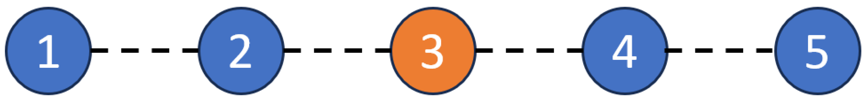
In order to illustrate the efficacy of the proposed discrete-time control architecture, consider a group of five agents on a line graph with the third agent being a leader. See Figure 1 for the graph formation chosen for the illustrative numerical examples of this paper.
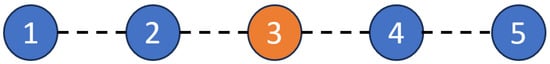
Figure 1.
Graph representation for an undirected line graph with five agents, where the third agent is the leader.
The coupled dynamics state parameter for each agent are selected according to the standard rule. In particular, the coupled dynamics parameters are selected as , , and . The known basis functions and unknown weights are assigned to create nonlinear and linear dynamics in the simulation. For the simulations, we set the uncertain weights as and the known basis functions are selected as , , , , and .
Here, we choose the nullspace and use the bounded command (i.e., ) such that . Thus, the expectation for convergences is that the first agent should converge to 0.5, the second agent should converge to 1, the third (the leader) agent should converge to 1.5, the fourth agent should converge to 1, and the fifth agent should converge to 0.5.
The update law requires the calculation of the learning rate , where the learning rate is defined as with being a free variable and is bound for the as given in Appendix A with selected and , and calculated . For the simulation and the calculation of value, we set the Lyapunov equation matrix R to 1 that yields . Note that the learning rate is restricted with for the stability of the closed-loop multiagent system; thus, we set the free variable to that yields a calculated learning rate value . We set the time step to (i.e., frequency to 5 [Hz] to show the discrete nature of the response of the multiagent system and this frequency is set to represent low-cost, small, and educational aerial or ground robots), where this results in the response having a leader convergence time of around 40 [s] that heavily depends on the learning rate, discrete-time step, user-assigned nullspace, and graph selection.
We set the control parameter to that satisfies rule defined in Section 2, where modified degree values are calculated as , , , , and . Here, the satisfies the rule and ensures that the eigenvalues of “” remains within the unit circle with , , , , and . Finally, all the initial conditions are set to zero.
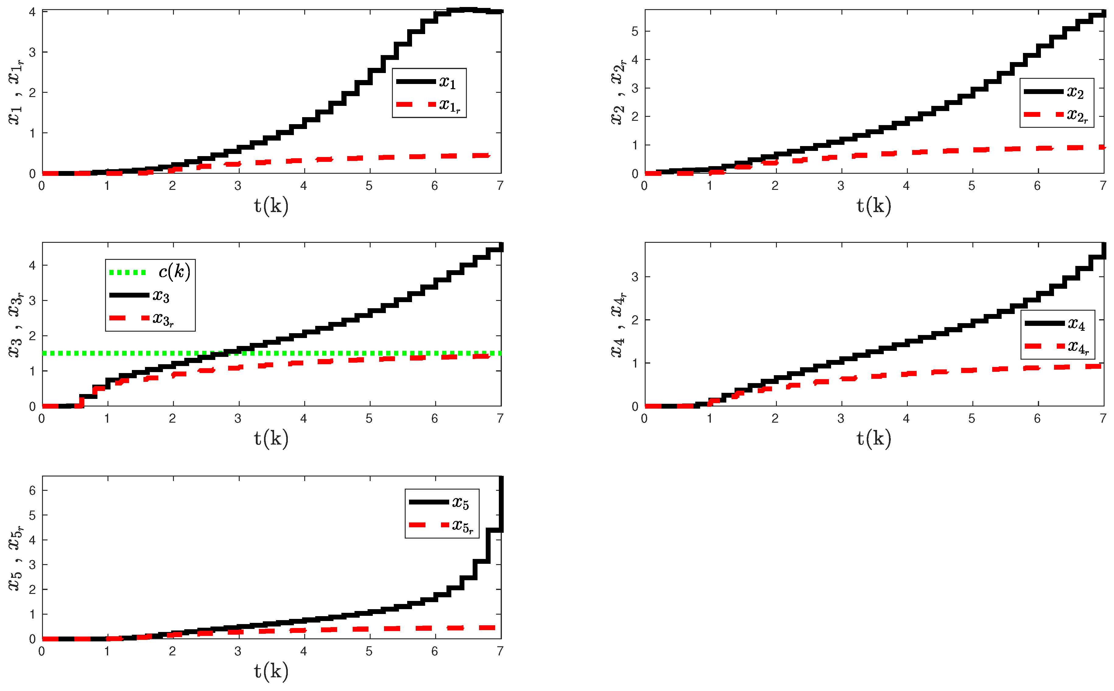
To motivate the necessity of the controller that is proposed in Section 3, we first simulate the uncertain multiagent system in the presence of the unmeasurable coupled dynamics with the proposed controller of Section 2. The simulation aims to replicate the conditions that agents might encounter, including the nonlinear and linear uncertainties and dynamic couplings that can significantly impact performance. Figure 2, Figure 3 and Figure 4 show the closed-loop system response with the proposed discrete-time adaptive control architecture given in Section 2.
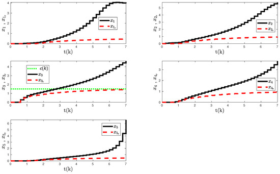
Figure 2.
Uncertain multiagent system response in the presence of coupled dynamics with the proposed discrete-time adaptive control method given in Section 2.

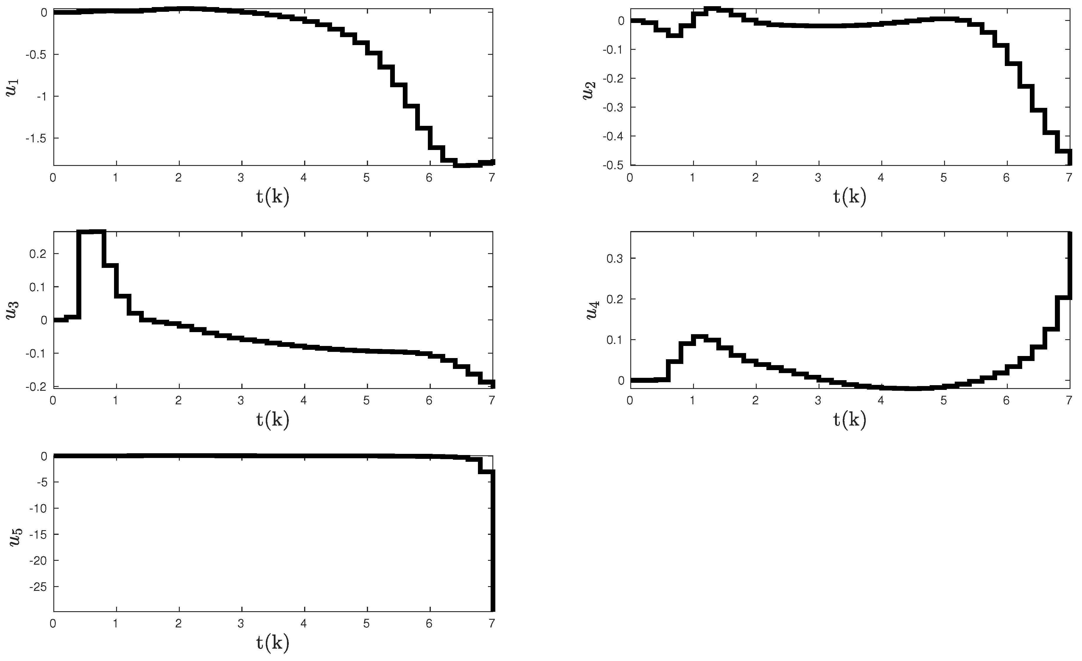
Figure 3.
Control inputs with the proposed discrete-time adaptive control method given in Section 2.
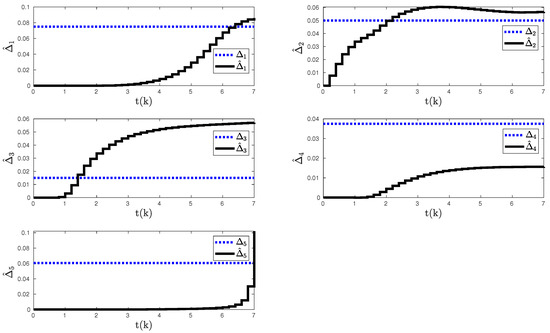
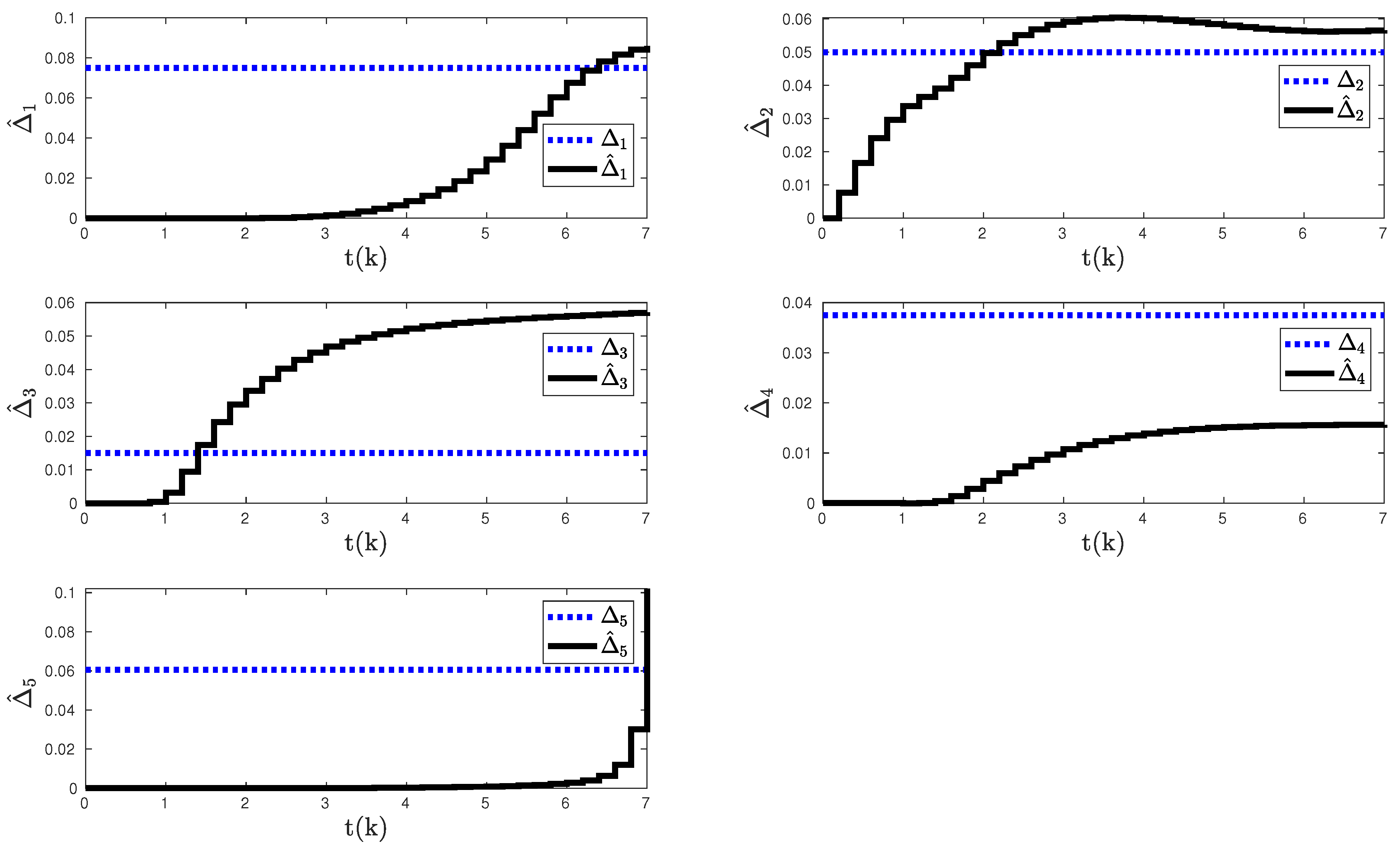
Figure 4.
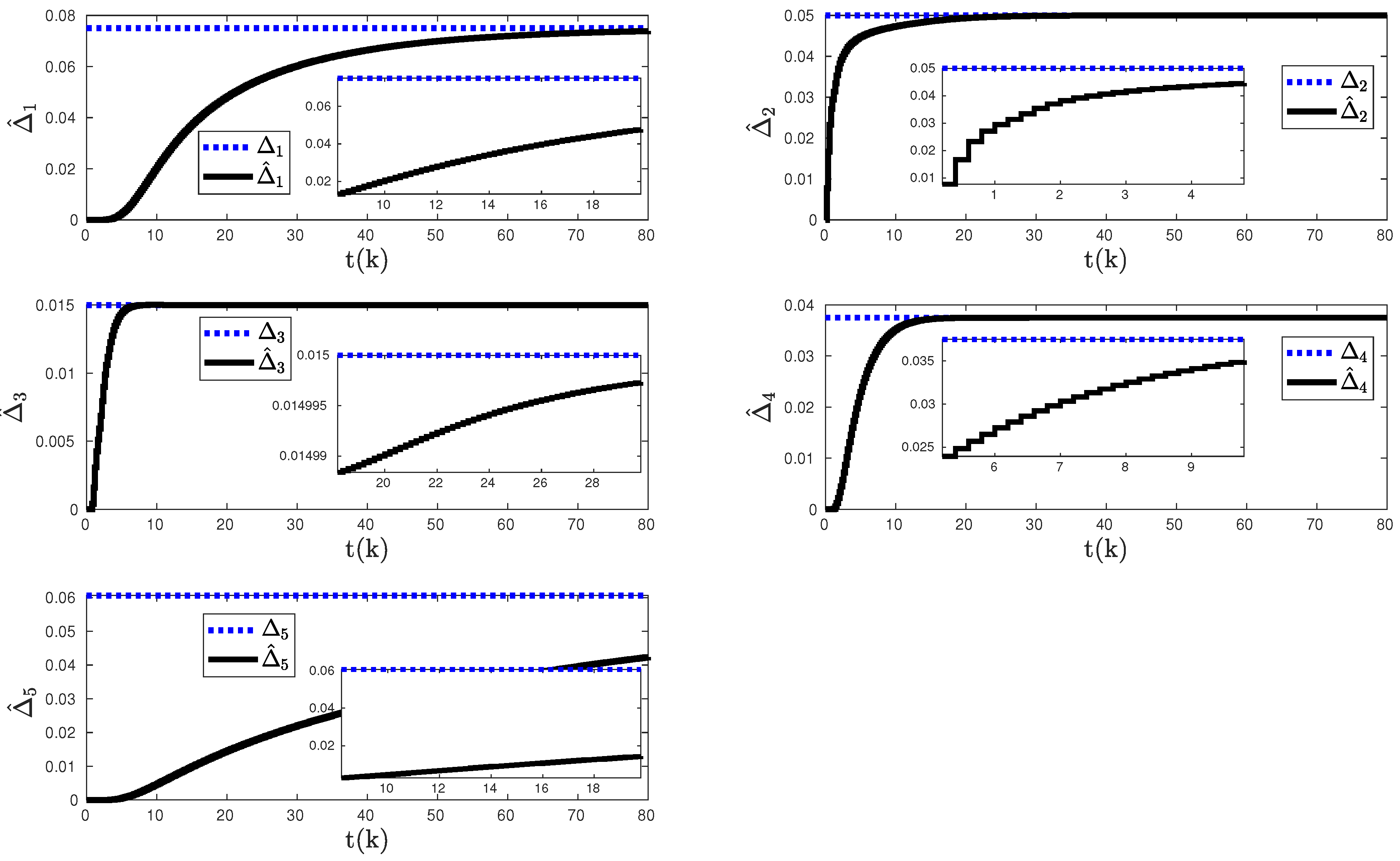
Agent-based uncertainty estimations of the proposed discrete-time adaptive control method given in Section 2.
However, as shown in Figure 2, Figure 3 and Figure 4, it is evident that the standard control strategy is insufficient for achieving convergence to the assigned positions and it even yields instability, highlighting the challenging nature of the task and the need for a more robust control solution. This lack of convergence is particularly noticeable in the tracking responses, which deviate from the desired trajectory and signal inadequate compensation for the uncertainties and coupled dynamics.
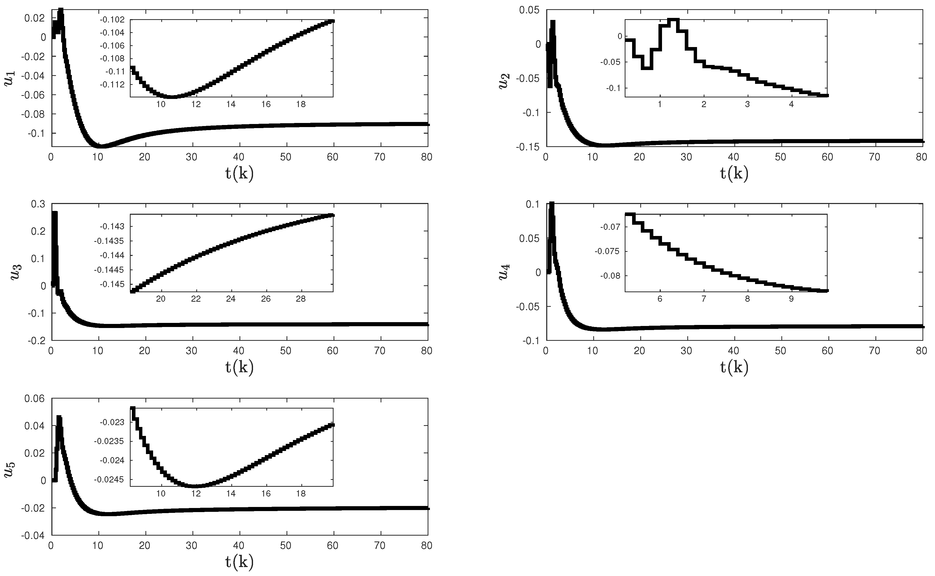
Building on these insights, we further implement the advanced discrete-time adaptive control architecture detailed in Section 3. This enhanced controller is specifically designed to address the instability in the earlier simulations, incorporating strategies for managing both the agent-based uncertainties and the coupled dynamics. Figure 5, Figure 6, Figure 7 and Figure 8 then show the closed-loop system response, control input, unknown weights estimates, and observer state, respectively, for each agent in the presence of the agent-based uncertainty and the coupled dynamics with the proposed discrete-time adaptive control architecture given in Section 3. These figures collectively illustrate an improvement over the initial results, with the system now successfully mitigating the adverse effects of uncertainties and coupled dynamics, as evidenced by the stabilized trajectories. Most notably, the convergence to the assigned positions is clearly achieved, validating the effectiveness of the proposed controller in Section 3.
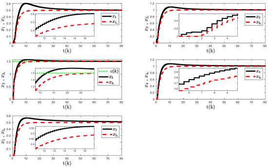
Figure 5.
Uncertain multiagent system response in the presence of coupled dynamics with the proposed discrete-time adaptive control method given in Section 3.
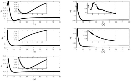
Figure 6.
Control inputs with the proposed discrete-time adaptive control method given in Section 3.
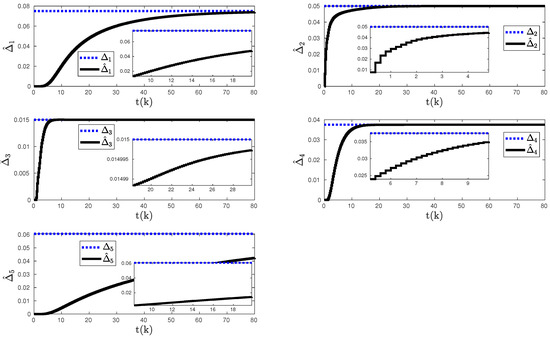
Figure 7.
Agent-based uncertainty estimations of the proposed discrete-time adaptive control method given in Section 3.
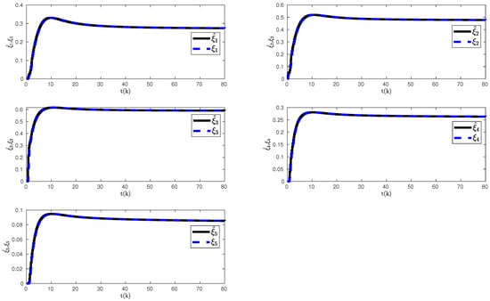
Figure 8.
Agent-based coupled dynamics of the proposed discrete-time adaptive control method given in Section 3.
In summary, the comparative analysis between the standard and proposed controller simulations serves as a compelling argument for the necessity of the proposed control architecture proposed in Section 3. The marked improvement in system performance and stability underscores the value and impact of the proposed discrete-time adaptive control solution in managing complex, uncertain multiagent systems.
5. Conclusions
This paper addresses the challenges and complexities associated with discrete-time architectures in the context of multiagent systems with uncertain scalar dynamics and coupled interactions. Specifically, the paper introduces a discrete-time adaptive control architecture with observer dynamics for managing unmeasurable coupled dynamics. Additionally, a user-assigned Laplacian matrix is incorporated to induce cooperative behaviors among multiple agents. The proposed control architecture is accompanied by Lyapunov analysis employing logarithmic and quadratic Lyapunov functions to guarantee asymptotic stability. Through an illustrative example, the paper demonstrates the effectiveness of the introduced control architecture, showcasing its ability to address uncertainties and coupled dynamics in multiagent systems. These contributions open avenues for further research in the development and application of adaptive control strategies in discrete-time scenarios.
The future research direction can include adding actuator dynamics and unknown control degradation to the multiagent system model and experimentally validating the theoretical results of this paper with the system with multiple robots to address real-world challenges. In addition, future research can include investigating the generalization of our control strategies to other graph types, such as directed, disconnected, or weekly connected graphs, aiming to address the specific challenges they present for multiagent systems. Finally, another future research direction is verifying and determining the convergence rate of the overall multiagent system that depends on learning rate, discrete-time step, user-assigned nullspace, and graph selection.
Author Contributions
Conceptualization, K.M.D.; Methodology, K.M.D. and I.A.A.; Validation, I.A.A.; Writing—original draft, I.A.A.; Writing—review & editing, I.A.A.; Supervision, K.M.D. All authors have read and agreed to the published version of the manuscript.
Funding
This research was supported by the National Aeronautics and Space Administration through the University of Central Florida’s NASA Florida Space Grant Consortium and Space Florida.
Data Availability Statement
The data presented in this study are available in this article.
Conflicts of Interest
The authors declare no conflict of interest.
Appendix A
In this appendix, the upper bound for is obtained. Given that , , and setting then the bound on can be written as
Then an upper bound for can be written as
where the Young’s inequality “” is used at the last step.
Appendix B
In this appendix, the below N is proven to be positive definite
Note that setting yields
Recall that ; and hence, “”. That concludes the positive definiteness of
Appendix C
In this appendix, the below matrix is proven to be positive semi-definite
To prove the positive semi-definiteness of the above matrix, one needs to prove that the minors of the matrix are positive semi-definite [44]. Let , ,and be the minors of given by
where is positive definite since and , and . To prove , one needs to use that is defined in Appendix B. Then one can conclude as
This concludes the proof that the matrix is positive semi-definite.
Appendix D
In this appendix, the below matrix is proven to be positive definite
with , , and . To prove the positive definiteness of the above matrix, one needs to prove that the minors of the matrix are positive semi-definite [44]. Let and be the minors of given by
Here, is positive definite since . Then setting yields
This concludes the proof that the matrix is positive definite.
References
- Olfati-Saber, R.; Fax, J.A.; Murray, R.M. Consensus and cooperation in networked multi-agent systems. Proc. IEEE 2007, 95, 215–233. [Google Scholar] [CrossRef]
- Ren, W.; Atkins, E. Distributed multi-vehicle coordinated control via local information exchange. Int. J. Robust Nonlinear Control 2007, 17, 1002–1033. [Google Scholar] [CrossRef]
- Mesbahi, M.; Egerstedt, M. Graph Theoretic Methods in Multiagent Networks; Princeton University Press: Princeton, NJ, USA, 2010. [Google Scholar]
- Lewis, F.L.; Zhang, H.; Hengster-Movric, K.; Das, A. Cooperative Control of Multi-Agent Systems: Optimal and Adaptive Design Approaches; Springer Science & Business Media: Berlin/Heidelberg, Germany, 2013. [Google Scholar]
- Rohrs, C.; Valavani, L.; Athans, M.; Stein, G. Robustness of continuous-time adaptive control algorithms in the presence of unmodeled dynamics. IEEE Trans. Autom. Control 1985, 30, 881–889. [Google Scholar] [CrossRef]
- Nguyen, N.; Urnes, J. Aeroelastic modeling of elastically shaped aircraft concept via wing shaping control for drag reduction. In Proceedings of the AIAA Atmospheric Flight Mechanics Conference, Minneapolis, MN, USA, 13–16 August 2012. [Google Scholar]
- Nobleheart, W.; Chakravarthy, A.; Nguyen, N. Active wing shaping control of an elastic aircraft. In Proceedings of the 2014 American Control Conference, Portland, OR, USA, 4–6 June 2014; pp. 3059–3064. [Google Scholar]
- Pequito, S.D.; Kar, S.; Aguiar, A.P. A Framework for Structural Input/Output and Control Configuration Selection in Large-Scale Systems. IEEE Trans. Automat. Contr. 2016, 61, 303–318. [Google Scholar]
- Hou, Z.G.; Cheng, L.; Tan, M. Decentralized robust adaptive control for the multiagent system consensus problem using neural networks. IEEE Trans. Syst. Man Cybern. Part B (Cybern.) 2009, 39, 636–647. [Google Scholar]
- Das, A.; Lewis, F.L. Distributed adaptive control for synchronization of unknown nonlinear networked systems. Automatica 2010, 46, 2014–2021. [Google Scholar] [CrossRef]
- Yucelen, T.; Egerstedt, M. Control of multiagent systems under persistent disturbances. In Proceedings of the 2012 American Control Conference (ACC), Montreal, QC, Canada, 27–29 June 2012; pp. 5264–5269. [Google Scholar]
- Yucelen, T.; Johnson, E.N. Control of multivehicle systems in the presence of uncertain dynamics. Int. J. Control 2013, 86, 1540–1553. [Google Scholar] [CrossRef]
- Wang, W.; Wen, C.; Huang, J. Distributed adaptive asymptotically consensus tracking control of nonlinear multi-agent systems with unknown parameters and uncertain disturbances. Automatica 2017, 77, 133–142. [Google Scholar] [CrossRef]
- Sarsilmaz, S.B.; Yucelen, T. A Distributed Adaptive Control Approach for Heterogeneous Uncertain Multiagent Systems. In Proceedings of the AIAA Guidance, Navigation, and Control Conference, Kissimmee, FL, USA, 8–12 January 2018. [Google Scholar]
- Dogan, K.M.; Gruenwald, B.C.; Yucelen, T.; Muse, J.A.; Butcher, E.A. Distributed adaptive control and stability verification for linear multiagent systems with heterogeneous actuator dynamics and system uncertainties. Int. J. Control 2018, 92, 2620–2638. [Google Scholar] [CrossRef]
- Pan, Y.; Ji, W.; Lam, H.K.; Cao, L. An improved predefined-time adaptive neural control approach for nonlinear multiagent systems. IEEE Trans. Autom. Sci. Eng. 2023. [Google Scholar] [CrossRef]
- Chen, L.; Liang, H.; Pan, Y.; Li, T. Human-in-the-loop consensus tracking control for UAV systems via an improved prescribed performance approach. IEEE Trans. Aerosp. Electron. Syst. 2023, 59, 8380–8391. [Google Scholar] [CrossRef]
- Dogan, K.M.; Yucelen, T.; Ristevki, S.; Muse, J.A. Distributed adaptive control of uncertain multiagent systems with coupled dynamics. In Proceedings of the 2020 American Control Conference (ACC), Denver, CO, USA, 1–3 July 2020; IEEE: Piscataway, NJ, USA, 2020; pp. 3497–3502. [Google Scholar]
- Dogan, K.M.; Yucelen, T.; Muse, J.A. Stability verification for uncertain multiagent systems in the presence of heterogeneous coupled and actuator dynamics. In Proceedings of the AIAA Scitech 2021 Forum, Online, 11–15 January 2021; p. 0530. [Google Scholar]
- Aly, I.A.; Dogan, K.M. Uncertain multiagent system in the presence of coupled dynamics: An asymptotic approach. In Proceedings of the AIAA SCITECH 2022 Forum, San Diego, CA, USA, 3–7 January 2022; p. 0359. [Google Scholar]
- DeVries, L.D.; Kutzer, M.D. Kernel design for coordination of autonomous, time-varying multi-agent configurations. In Proceedings of the 2016 American Control Conference, Boston, MA, USA, 6–8 July 2016; IEEE: Piscataway, NJ, USA, 2016; pp. 1975–1980. [Google Scholar]
- DeVries, L.; Sims, A.; Kutzer, M.D. Kernel Design and Distributed, Self-Triggered Control for Coordination of Autonomous Multi-Agent Configurations. Robotica 2018, 36, 1077–1097. [Google Scholar] [CrossRef]
- Tran, D.; Yucelen, T. On new Laplacian matrix with a user-assigned nullspace in distributed control of multiagent systems. In Proceedings of the 2020 American Control Conference (ACC), Denver, CO, USA, 1–3 July 2020. [Google Scholar]
- Dogan, K.M.; Yucelen, T. Distributed Adaptive Control for Uncertain Multiagent Systems with User-Assigned Laplacian Matrix Nullspaces. In Proceedings of the 2021 IEEE Conference on Control Technology and Applications (CCTA), Online, 9–11 August 2021. [Google Scholar]
- Kurttisi, A.; Aly, I.A.; Dogan, K.M. Coordination of Uncertain Multiagent Systems with Non-Identical Actuation Capacities. In Proceedings of the 2022 IEEE 61st Conference on Decision and Control (CDC), Cancun, Mexico, 6–9 December 2022; IEEE: Piscataway, NJ, USA, 2022; pp. 3947–3952. [Google Scholar]
- Aly, I.A.; Kurttisi, A.; Dogan, K.M. An Observer-Based Distributed Adaptive Control Algorithm for Coordination of Multiagent Systems in the Presence of Coupled Dynamics. In Proceedings of the 2023 American Control Conference (ACC), San Diego, CA, USA, 31 May–2 June 2023; pp. 521–526. [Google Scholar]
- Santillo, M.A.; Bernstein, D.S. Adaptive control based on retrospective cost optimization. J. Guid. Control Dyn. 2010, 33, 289–304. [Google Scholar] [CrossRef]
- Goodwin, G.; Ramadge, P.; Caines, P. Discrete-time multivariable adaptive control. IEEE Trans. Autom. Control 1980, 25, 449–456. [Google Scholar] [CrossRef]
- Kanellakopoulos, R. A discrete-time adaptive nonlinear system. In Proceedings of the American Control Conference, Baltimore, MD, USA, 29 June–1 July 1994; pp. 867–869. [Google Scholar]
- Venugopal, R.; Rao, V.; Bernstein, D. Lyapunov-based backward-horizon discrete-time adaptive control. Adapt. Contr. Sig. Proc. 2003, 17, 67–84. [Google Scholar]
- Hayakawa, T.; Haddad, W.M.; Leonessa, A. A Lyapunov-based adaptive control framework for discrete-time non-linear systems with exogenous disturbances. Int. J. Control 2004, 77, 250–263. [Google Scholar] [CrossRef]
- Akhtar, S.; Venugopal, R.; Bernstein, D.S. Logarithmic Lyapunov functions for direct adaptive stabilization with normalized adaptive laws. Int. J. Control 2004, 77, 630–638. [Google Scholar] [CrossRef]
- Johansson, R. Global Lyapunov stability and exponential convergence of direct adaptive control. Int. J. Control 1989, 50, 859–869. [Google Scholar] [CrossRef]
- Johansson, R. Supermartingale analysis of minimum variance adaptive control. Control-Theory Adv. Technol. 1995, 10, 993–1013. [Google Scholar]
- Haddad, W.M.; Hayakawa, T.; Leonessa, A. Direct adaptive control for discrete-time nonlinear uncertain dynamical systems. In Proceedings of the American Control Conference, Anchorage, AK, USA, 8–10 May 2002; pp. 1773–1778. [Google Scholar]
- Hoagg, J.B.; Santillo, M.A.; Bernstein, D.S. Discrete-time adaptive command following and disturbance rejection with unknown exogenous dynamics. IEEE Trans. Autom. Control 2008, 53, 912–928. [Google Scholar] [CrossRef]
- Li, H.; Wu, Y.; Chen, M. Adaptive fault-tolerant tracking control for discrete-time multiagent systems via reinforcement learning algorithm. IEEE Trans. Cybern 2020, 51, 1163–1174. [Google Scholar] [CrossRef] [PubMed]
- Jiang, Y.; Fan, J.; Gao, W.; Chai, T.; Lewis, F.L. Cooperative adaptive optimal output regulation of nonlinear discrete-time multi-agent systems. Automatica 2020, 121, 109149. [Google Scholar] [CrossRef]
- Yildirim, E.; Yucelen, T. Discrete-Time Control of Multiagent Systems with a Misbehaving Node. In Proceedings of the 2022 American Control Conference (ACC), Atlanta, GA, USA, 8–10 June 2022; IEEE: Piscataway, NJ, USA, 2022; pp. 48–53. [Google Scholar]
- Aly, I.A.; Dogan, K.M. Discrete-Time Adaptive Control Algorithm for Coordination of Multiagent Systems in the Presence of Coupled Dynamics. In Proceedings of the 2023 IEEE/RSJ International Conference on Intelligent Robots and Systems (IROS), Detroit, MI, USA, 1–5 October 2023; IEEE: Piscataway, NJ, USA, 2023; pp. 5366–5371. [Google Scholar]
- Godsil, C.D.; Royle, G. Algebraic Graph Theory; Springer: New York, NY, USA, 2001. [Google Scholar]
- Haddad, W.M.; Chellaboina, V. Nonlinear Dynamical Systems and Control: A Lyapunov-Based Approach; Princeton University Press: Princeton, NJ, USA, 2008. [Google Scholar]
- Topsok, F. Some bounds for the logarithmic function. Inequal. Theory Appl. 2006, 4, 137. [Google Scholar]
- Bhatia, R. Positive Definite Matrices; Princeton University Press: Princeton, NJ, USA, 2009. [Google Scholar]


Disclaimer/Publisher’s Note: The statements, opinions and data contained in all publications are solely those of the individual author(s) and contributor(s) and not of MDPI and/or the editor(s). MDPI and/or the editor(s) disclaim responsibility for any injury to people or property resulting from any ideas, methods, instructions or products referred to in the content. |
© 2024 by the authors. Licensee MDPI, Basel, Switzerland. This article is an open access article distributed under the terms and conditions of the Creative Commons Attribution (CC BY) license (https://creativecommons.org/licenses/by/4.0/).