Positioning Improvement with Multiple GPS Receivers Based on Shallow Asymmetric Neural Network

Abstract

A positioning system in a specific space is for the purpose of determining the location of an object. The Global Positioning System (GPS) is the most popular and valuable development for classical navigation. However, it may not always be precise and available due to the effects of multi-path propagation and signal attenuation. Thus, we need some additional skills to keep its stability and accuracy or improve its performance. Based on the technique of neural networks, the positioning information from multiple GPS receivers is composed to obtain a better version which is more accurate and stable and thus can be applied to advanced applications. Particularly, the concepts of shallow and asymmetric neural networks are used in this work. Our design possesses fewer hidden layers via the former property and further reduces the connections of classical Fully Connected Neural Networks (FCNNs) via the latter property. Hence, it takes very little time to realize the training and predicting procedures. Also, it will help promote several works in practice, such as the implementation of embedded systems. Finally, a practical test, called the vehicular road test, is utilized to guarantee the level of confidence in the improvement of our algorithm.

1. Introduction

Recently, research on smart vehicles has become one of the most popular and important topics in the world. Since those advanced applications for smart vehicles need more accurate and stable perceptions, various improvements for distinct sensors, e.g., Global Positioning System (GPS), inertial measurement unit (IMU), odometer, camera, ultrasound, lidar, and so forth, are presented in the literature.

A positioning system in a specific space is for the purpose of determining the location of an object. From interplanetary systems to workspace systems for various applications, both outdoors and indoors, there are plenty of positioning techniques presented in the literature [1]. GPS is the most popular and valuable development for classical navigation. However, it may not always be precise and available due to the effects of multi-path propagation and signal attenuation [2,3,4,5,6,7]. Thus, we need some additional skills to keep its stability and accuracy or even improve its performance to be qualified for the advanced applications of smart vehicles, e.g., advanced navigation, accurate tracking, precise timing, and so on.

In this paper, we reconsider the GPS positioning issue. Based on the technique of neural networks, the positioning information from multiple GPS receivers can be composed to obtain a better version which is more accurate and stable and thus can be applied to advanced applications. Noteworthily, there are distinct research studies for the GPS positioning topic proposed in the literature, e.g., sensor fusion, the Differential Global Positioning System (DGPS), and so on. However, most of the aforementioned ideas need extra devices to realize improvements. For example, sensor fusion means incorporating different sensor information into the GPS information and then obtaining better positioning information [8,9,10]. In [10], the authors introduce many integrated navigation systems, e.g., air, land, and underwater applications. Some of them do not use any GPS receivers. This means that a design only considering GPS receivers is a flexible part for different positioning issues that may adopt various sets of positioning devices. DGPS utilizes fixed reference stations to broadcast the difference information between the positions indicated by GPS receivers and known fixed reference positions [11]. Consequently, this motivates us to consider whether only using multiple GPS receivers to realize the positioning improvement is possible or not. Notably, various approaches in the literature have employed fully connected networks for information fusion. However, in contrast to the fully connected network paradigm, this study adopts the principles of shallow and asymmetric neural networks. These concepts mitigate challenges related to inefficient training and overfitting, facilitating practical applications such as the implementation of embedded systems.

According to our experiments, the statistics for GPS raw data do not fit the simple normal distribution. Hence, if we use such a distribution to simulate the noise/error, then obtaining an exact solution to obtain a better positioning performance is impossible. Also, it is not a simple problem of linear or polynomial regression. Thus, we use the MLP (Multi-Layer Perceptron) to design our method, which can be applied to complex nonlinear problems. Most important of all, a practical test, called the vehicular road test, is utilized to guarantee the level of confidence in the improvement of our algorithm. This paper is organized as follows: first, several necessary preliminaries related to our work are introduced. Next, we start to address our method, which is based on the MLP, to deal properly with the GPS positioning issue in real scenarios. Then, the experimental results, as well as corresponding discussion, are provided. Finally, the last section concludes this work and discusses some feasible future works.

2. Preliminaries

2.1. GPS Receiver and NMEA Sentence

The NMEA (National Marine Electronics Association) sentence is a data specification for communication between marine electronics, e.g., echo sounder, sonar, anemometer, gyro-compass, autopilots, GPS receiver, and so forth. It has been defined and updated by the National Marine Electronics Association [12]. Nowadays, the NMEA sentence has become the most common format for data output of all GPS receivers [13,14].

The standard uses the serial communication protocol based on ASCII (American Standard Code for Information Interchange), which defines how data are transmitted at a time. For example, we can use the sentence $GPGGA to obtain information on latitude, longitude, fix quality, checksum, and so forth. Noteworthily, via the fields of fixed quality and checksum in the sentence, only the valid positioning messages without transmission errors will be further processed.

2.2. Conversion/Transformation between Coordinates

Generally, we can obtain information on latitude, longitude, and altitude from a GPS receiver, and these are named the geodetic coordinates. However, it is not clear or intuitive for general units of measurement, e.g., the meter, centimeter, and so forth. Therefore, conversion/transformation between different coordinates is needed.

A geographic coordinate conversion is a translation between different coordinate formats that are referenced to the same geodetic datum. A geographic coordinate transformation is a translation between different geodetic data [15]. Both are needed if we want to represent the position of an object or the distance between two objects with the metric system. Particularly, the geodetic coordinates are first translated into the geocentric coordinates, which are also known as the ECEF (Earth-Centered, Earth-Fixed) coordinates. Then, we can translate the ECEF coordinates into local tangent plane coordinates, which are also known as the ENU (East-North-Up) coordinates and are measured in metric units [16].

The former can be realized via Equations (1)–(4):

$$X=\left(N\left(\varphi \right)+h\right)cos\varphi cos\lambda ,$$

(1)

$$Y=\left(N\left(\varphi \right)+h\right)cos\varphi sin\lambda ,$$

(2)

$$Z=\left(\frac{b^2}{a^2}N\left(\varphi \right)+h\right)sin\varphi ,$$

(3)

$$N\left(\varphi \right)=\frac{a^2}{\sqrt{a^2{\left(cos\varphi \right)}^2+b^2{\left(sin\varphi \right)}^2}},$$

(4)

where $\varphi$ is the latitude, $\lambda$ is the longitude, h is the altitude, a is the equatorial radius, and b is the polar radius. Then, the latter can be realized via Equation (4):

$$\left[\begin{array}{c}x\\ y\\ z\end{array}\right]=\left[\begin{array}{ccc}-sin{\lambda }_r& cos{\lambda }_r& 0\\ -sin{\varphi }_{r}cos{\lambda }_r& -sin{\varphi }_{r}sin{\lambda }_r& cos{\varphi }_r\\ cos{\varphi }_{r}cos{\lambda }_r& cos{\varphi }_{r}sin{\lambda }_r& sin{\varphi }_r\end{array}\right]\left[\begin{array}{c}{X}_p-X_r\\ Y_p-Y_r\\ Z_p-Z_r\end{array}\right],$$

(5)

where $\left(X_r,Y_r,Z_r\right)$ are the coordinates of the reference point, $\left(X_p,Y_p,Z_p\right)$ are the coordinates of the object, $\varphi$ is the latitude, and $\lambda$ is the longitude.

2.3. Robot Operating System and Rosbag

ROS (Robot Operating System) is a flexible framework which is a collection of libraries, tools, and conventions to simplify the aim of designing complex and robust robot applications across different platforms. Since creating robots is very hard, no single laboratory or institution can achieve this on its own. Thus, ROS was built to encourage collaborative development [17]. For instance, one laboratory contributes a system for producing maps, one institution designs the navigation algorithm based on the maps, and another organization controls the robots based on the navigation.

In ROS, a process or node within a graph is linked by at least one edge, commonly referred to as a topic. Therefore, a node can communicate with another node (or other nodes) through the topic(s). Obviously, this is the peer-to-peer communication of the decentralized network.

In this paper, the most important package for us is rosbag, which is for recording from and playing back to ROS topics. Particularly, it is intended to be high performance and avoid the deserialization and re-serialization of messages [18]. Accordingly, via rosbag, we can deal properly with the issue of the message stream easily, i.e., with the positioning information from different GPS receivers at the same time.

2.4. Neural Network

A neural network (NN) is a machine learning (ML) model that is inspired by the architectures of biological neurons. Due to its properties, NN can be collocated with other technologies to deal with complex and large issues, e.g., optimization, classifying images, speech recognition, and so forth [19,20,21,22]. Obviously, it is versatile, powerful, and scalable.

In the area of NNs, one of the simplest architectures is the Perceptron. For every neuron, the inputs and outputs are numbers. Furthermore, every input is associated with a weight as well as an extra bias. Next, the weighted sum is applied to an activation function to produce the output. Noteworthily, the Multi-Layer Perceptron (MLP) is an improved version of the Perceptron, which is constructed from one input layer, hidden layer(s), and one output layer, where each layer except the output layer is fully connected to the next layer. Note that the hidden layer is formed with the concept of the Perceptron [19,20,21,22]. The computation of the Perceptron is presented in Equations (6) and (7):

$${\beta }_i={\alpha }_{n-1}{\omega }_{n-1}+\dots +{\alpha }_0{\omega }_0+bia{s}_i,$$

(6)

$${\gamma }_i=activatio{n}_i\left({\beta }_i\right),$$

(7)

where ${\alpha }_i$ is the input, ${\omega }_i$ is the weight of ${\alpha }_i$, $bia{s}_i$ is the bias, ${\beta }_i$ is the weighted sum, and ${\gamma }_i$ is the output produced from the activation function $activatio{n}_i\left(\right)$.

Due to the effects of signal attenuation and multi-path propagation [2,3,4,5,6,7], the improvement of GPS positioning is not a simple linear issue. Hence, since MLP can be applied to complex nonlinear problems [19,20,21,22], this is the motivation for us to design a new architecture including an NN to refine the GPS positioning information. Moreover, for the reason of real-time operation, we will only consider the straightforward design of the NN instead of the complex and deep one. Here, the concepts of shallow and asymmetric neural networks are used in this work. More specifically, the former property obviously brings fewer trainable parameters. Then, the latter performs as well via reducing the connections of classical fully connected networks.

3. The Improvement Procedure

In the experiments, we first gather the statistics for the GPS raw data in various scenarios to check the properties of different GPS receivers. According to the raw data, the statistics for GPS raw data do not fit the simple normal distribution (the detailed information will be presented in the next section). Hence, if we use such a distribution to simulate the noise/error, obtaining an exact solution to obtain a better positioning performance is hard, even impossible. Next, we also observe an interesting phenomenon: even though the GPS receivers are the same product model, they still obtain positioning information with drastically different properties. The intuition is that there may be some hardware component tolerances in these GPS receivers. Hence, the positioning issue of multiple GPS receivers is not a simple problem of linear or polynomial regression. Thus, we use the MLP (Multi-Layer Perceptron) to design our method, which can be applied to complex nonlinear problems.

Before the training procedure of the neural network, we define several prefilters for the purpose of filtering unreasoned positioning raw data that are influenced by multi-path propagation and signal attenuation. If these influenced data are adopted to train the neural network, the performance of such a neural network will be influenced as well. Hence, choosing appropriate prefilters is important for the machine learning topic. Again, the results and comparisons of utilizing different prefilters before the training procedure will be presented in the next section.

Now, we begin to elaborate our algorithm, which is the positioning improvement procedure with multiple GPS receivers based on the neural network and presented in Algorithm 1. Foremost, several variables are defined: x is the number of GPS receivers used in the experiments and the amount of positioning data received at a time (line 1), X is the data set containing the positioning data received from GPS receivers at a time (line 2), y is the number of positioning data after filtering out unreasoned parts at a time (line 3), Y is the data set containing the positioning data after filtering out unreasoned parts at a time (line 4), $model$ is the model used in the experiments (line 5), and $position$ is the improvement position (line 6).

In the initial phase, the position of each GPS receiver is initialized ahead (line 7). This is a critical step since the relative position of each GPS receiver will affect the estimation of the performance of our positioning system. Upon receiving X from all GPS receivers at a time, we filter X via the prefilter(s) to obtain Y (line 8). Note that what the prefilters accomplish is presented in Algorithm 2 and will be detailed later. After receiving enough Y, we can start to train the model (line 9).

Next, in the implementation phase, since the model is trained, upon receiving X from all GPS receivers at a time, after filtering X via the prefilter(s) and obtaining Y (line 10), we can utilize the trained model to obtain better positioning information (line 11).

Algorithm 1: Positioning improvement procedure with multiple GPS receivers.
	variables:		initial phase:
1	x: the number of receivers and the amount of positioning data received at a time;	7	initialize the position of each receiver; upon receiving X from receivers at a time;
2	X: the data set contains the positioning data received from the receivers at a time;	8	filter X via prefilter(s) and obtain Y; upon receiving sufficient amount of Y;
3	y: the number of positioning data after filtering out unreasoned parts at a time;	9	train model implementation phase: upon receiving X from receivers at a time:
4	Y: the data set contains the positioning data after filtering out unreasoned parts at a time;	10	filter X via prefilter(s) and obtain Y;
5	model: the model used in the experiment;	11	position← predict (model, Y);
6	position: the improvement position;

On the other hand, in Algorithm 2, we start to detail what the prefilters accomplish. Similarly, several variables are defined ahead: x is the number of GPS receivers used in the experiments and the amount of positioning data received at a time (line 1), X is the data set containing the positioning data received from GPS receivers at a time (line 2), y is the number of positioning data after filtering out unreasoned parts at a time (line 3), Y is the data set containing the positioning data after filtering out unreasoned parts at a time (line 4), $bias$ is the difference between the positioning data and the ground truth (line 5), and $average$ is the average of positioning data in the data set (line 6). Note that the aforementioned bias and average are both two-dimensional vectors since the positioning information obtained from the GPS receivers includes latitude and longitude information.

Next, for the first prefilter, we input X, perform nothing, and output Y (lines 7–9). This means X and Y are the same. For the second prefilter, the bias of each positioning data in X is estimated and removed (lines 10 and 11), and then these positioning data are stored in Y and outputted (lines 12 and 13). Noteworthily, since the bias of each positioning datum from every GPS receiver varies from the environment and time, we can only estimate the bias via stopping at a fixed position before the experiments. Obviously, after only removing the bias in the abovementioned manner, the positioning data are not accurate and stable enough. For the third prefilter, $average$ is set to the average of all positioning data in X (lines 14 and 15). Then, we discard some data in X that are furthest from $average$ (line 16). Finally, the residual parts are stored in Y and outputted (lines 16 and 17). Therefore, the third prefilter is the sole one among all prefilters that will change the amount of positioning data.

Algorithm 2: Various prefilters for our positioning improvement procedure.
	variables		prefilter 01
1	x: the number of receivers and the number of positioning data received at a time	7	input X
		8	do nothing
2	X: the data set contains the positioning data received from the receivers at a time;	9	output Y; prefilter 02:
3	y: the number of positioning data after filtering out unreasoned parts at a time;	10	input X;
		11	bias← estimate bias
4	Y: the data set contains the positioning data after filtering out unreasoned parts at a time;	12	Y← remove bias from all data in X;
		13	output Y; prefilter 03:
5	bias: the difference between the positioning data and the ground truth;	14	input X;
		15	average ← average X;
6	average: the average of positioning data in the data set;	16	Y ← discard some data in X that are furthest from average;
		17	output Y;

4. Experimental Results

In this section, we start to detail the experiments. All experimental settings are listed as follows:

• In Figure 1 and Figure 2, six GPS receivers (BU-353S4 [13]) are mounted on the vehicle.
• In Figure 1 and Figure 2, one RTK-GPS receiver (PP7E1 [14]) is also mounted on the vehicle, which is treated as the real-time ground truth.
• The positioning data of BU-353S4 is provided at a rate of 1 message per second, and that of PP7E1 is from 1 to 100 messages per second. For the consistency of the data stream, it is also set to one for the latter.
• rosbag of ROS is utilized to record all positioning data from the above seven receivers.
• Three scenarios are adopted for our experiments, i.e., stopping in the parking lot, driving slowly in the parking lot, and driving on the road.
• The trajectories of the parking lot and driving road are shown in Figure 3 and Figure 4, where the former is about 0.28 km and the latter 4.03 km.
• The purpose of stopping in the parking lot is to estimate the bias of each GPS receiver separately mounted on the vehicle.
• After collecting enough positioning data by driving slowly in the parking lot and driving on the road, the data are split into two portions: 80% for the training procedure and 20% for the testing procedure. Using different data sets to train a machine learning model and validate its performance is a crucial step in building a robust and reliable model that performs well on new data.
• The specification of the experimental computer:

  -

  CPU: Intel Core i7-9700;

  -

  GPU: NVIDIA GeForce RTX 2080 8 GB;

  -

  RAM: 16 GB 3200 MHz.

• TensorFlow 2.12 [23] is used in this paper for all machine learning operations.

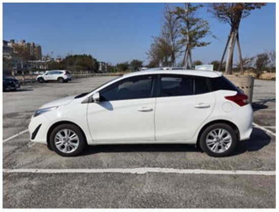
Figure 1. The vehicle for the vehicular road test.

Figure 1. The vehicle for the vehicular road test.

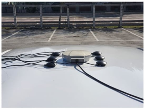
Figure 2. All GPS receivers are mounted on the vehicle.

Figure 2. All GPS receivers are mounted on the vehicle.

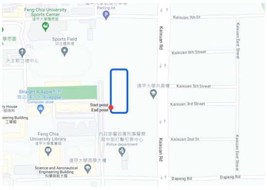
Figure 3. The trajectory of the parking lot.

Figure 3. The trajectory of the parking lot.

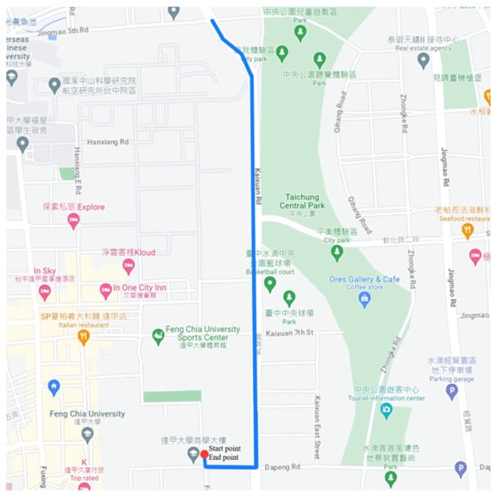
Figure 4. The trajectory of the driving road.

Figure 4. The trajectory of the driving road.

Firstly, we gather statistics for the bias of each GPS receiver via stopping in the parking lot, and the results are shown in Figure 5. According to the results, we can observe that even if the GPS receivers are the same product model, they still obtain positioning information with drastically different properties. The intuition is that there may be some hardware component tolerances in these GPS receivers. Hence, the positioning issue of multiple GPS receivers is not a simple problem of linear or polynomial regression. Thus, the neural network is adopted to design our method, which can deal properly with complex nonlinear problems. Noteworthily, the average bias of each GPS receiver is correspondingly 6.50 cm, 6.10 cm, 6.28 cm, 6.69 cm, 6.46 cm, and 6.66 cm. These values will be adopted for the second prefilter of our algorithm afterward.

Next, we drive the vehicle slowly in the parking lot, which is an open-sky environment. The statistics for the error of each GPS receiver with the same trajectory during the five rounds are shown in the following figures. Obviously, on the basis of the results in Figure 6, Figure 7, Figure 8, Figure 9, Figure 10 and Figure 11, the positioning information also has drastically different properties. This situation is consistent with our inference, which motivated us to start this study. Notice that the definitions of the terms bias and error between a receiver and the ground truth are the same, the former is often used to describe the inaccurate part of a sensor, and the latter is often utilized to describe the results of an experiment.

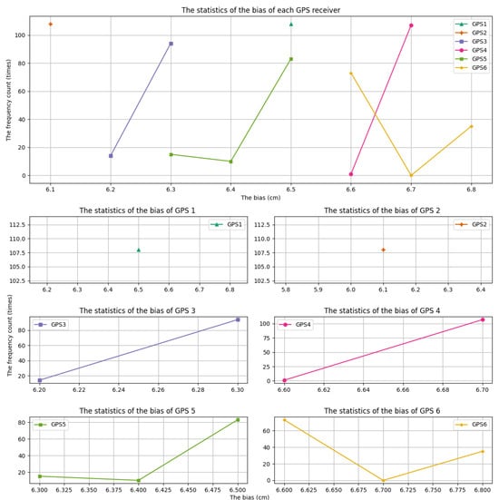
Figure 5. The statistics for the bias of each GPS receiver.

Figure 5. The statistics for the bias of each GPS receiver.

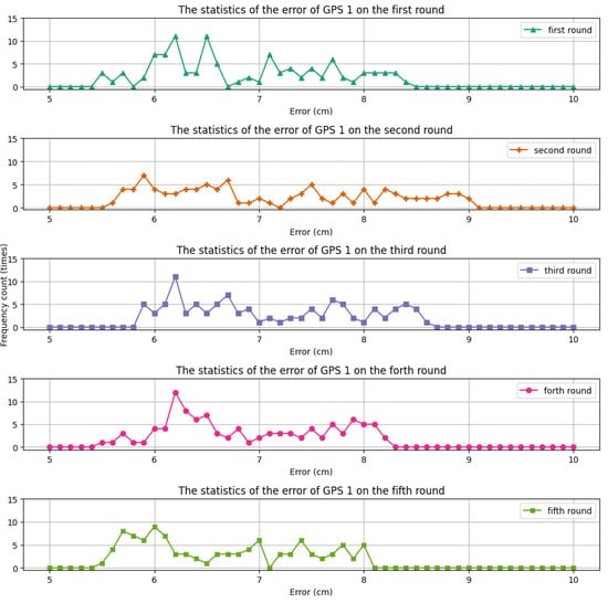
Figure 6. The statistics for the error of the first GPS receiver on all rounds.

Figure 6. The statistics for the error of the first GPS receiver on all rounds.

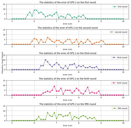
Figure 7. The statistics for the error of the second GPS receiver on all rounds.

Figure 7. The statistics for the error of the second GPS receiver on all rounds.

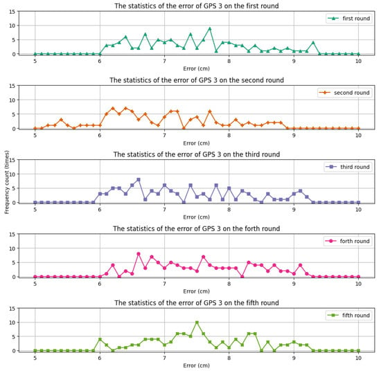
Figure 8. The statistics for the error of the third GPS receiver on all rounds.

Figure 8. The statistics for the error of the third GPS receiver on all rounds.

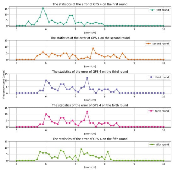
Figure 9. The statistics for the error of the fourth GPS receiver on all rounds.

Figure 9. The statistics for the error of the fourth GPS receiver on all rounds.

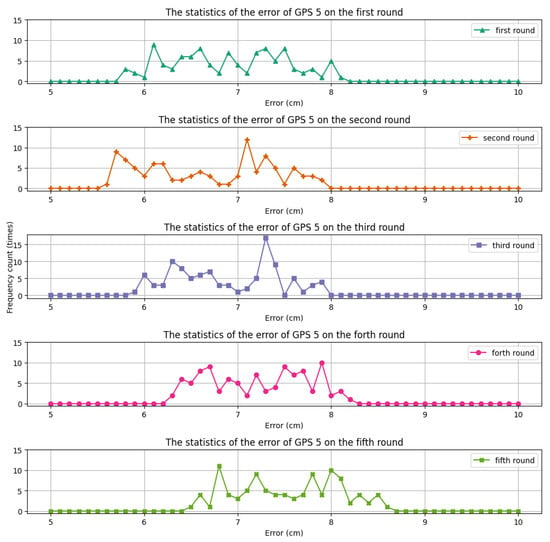
Figure 10. The statistics for the error of the fifth GPS receiver on all rounds.

Figure 10. The statistics for the error of the fifth GPS receiver on all rounds.

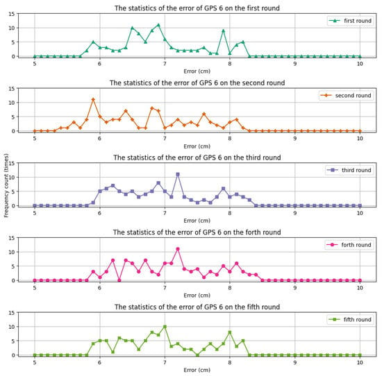
Figure 11. The statistics for the error of the sixth GPS receiver on all rounds.

Figure 11. The statistics for the error of the sixth GPS receiver on all rounds.

On the basis of the algorithm in Algorithm 1 and prefilters in Algorithm 2, several procedures are designed and shown in Figure 12. More specifically, we integrate different prefilters with the algorithm to conduct our experiments and estimate their performance. For example, in procedure 04 shown in Figure 13, all raw data are foremost filtered via prefilter 02 and prefilter 03 sequentially and then combined to form the improved version via the sole algorithm.

On the other hand, the design of the neural network is presented in Figure 14, where the inputs are 4 or 6 pieces of positioning data, and the output is the sole improvement version. Moreover, the number shown in each layer is utilized to represent the number of neurons in this layer. Accordingly, the number of trainable parameters in our designs is extremely small, i.e., 458 and 414. Notice that since different prefilters will produce various numbers of outputs as the inputs to the succeeding neural network, our model is designed flexibly for different numbers of inputs. Particularly, the operations of the information of latitude and longitude are separated in the first half, while they are integrated in the second half. Specifically, the architecture does not rely on a fully connected network. Instead, this study employs the concepts of shallow and asymmetric neural networks. These concepts serve to mitigate issues related to inefficient training and overfitting while also facilitating practical applications such as implementation on embedded systems. Next, the detailed settings of such a neural network are given below:

• Learning rate: 0.0001;
• $Bet{a}_1$: 0.999;
• $Bet{a}_2$: 0.99999;
• Epsilon: None;
• Decay: 0.000000001;
• Optimizer: Adam;
• Activation function: Relu and linear.

Figure 12. The design of the procedure on the basis of Algorithm 1 and prefilters in Algorithm 2.

Figure 12. The design of the procedure on the basis of Algorithm 1 and prefilters in Algorithm 2.

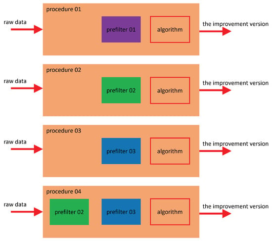
Figure 13. The expanded procedures from Figure 12.

Figure 13. The expanded procedures from Figure 12.

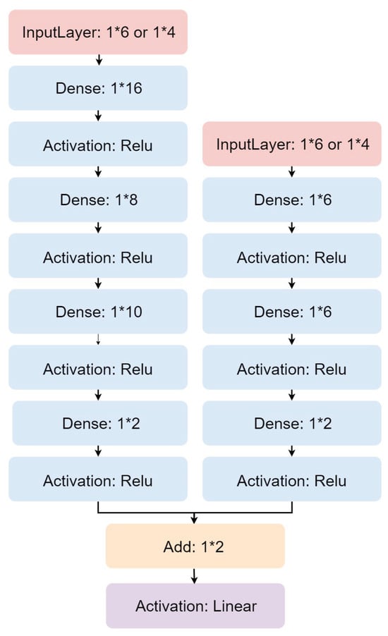
Figure 14. The design of the neural network.

Figure 14. The design of the neural network.

The experimental results are illustrated in

Table 1. The experimental results among all procedures.

	Error While Driving Slowly in the Parking Lot (m)	Standard Deviation While Driving Slowly in the Parking Lot (m)	Error While Driving on the Road (m)	Standard Deviation While Driving on the Road (m)
GPS raw data	7.38	0.88	7.64	3.00
procedure 01	0.96	0.47	3.48	1.46
procedure 02	0.77	0.39	3.29	1.40
procedure 03	0.78	0.36	3.34	1.44
procedure 04	0.75	0.36	3.26	1.42

. Foremost, we can observe that the errors while driving slowly in the parking lot and driving on the road are both more than 7 m. Particularly, the standard deviation while driving on the road is especially terrible. The intuition is that the vehicle performs stop-and-go while driving on the road, and there are several types of interference on the road, e.g., trees, traffic signs, and so on.

Then, in procedure 01, where only the neural network presented in Figure 12 is adopted, we can see that the positioning performance is obviously better. Namely, the error is reduced to 0.96 m while driving slowly in the parking lot and 3.48 m while driving on the road. Similarly, the standard deviation is reduced to 0.47 m while driving slowly in the parking lot and 1.46 m while driving on the road. Hence, we can realize that the property of the neural network works well for obtaining a better version, which is only composed of the raw data from six GPS receivers.

Next, the positioning performance is further improved via three different procedures. Particularly, in addition to the aforementioned neural network, procedure 02, procedure 03, and procedure 04 additionally include respective prefilters. Note that the prefilter in procedure 04 is the prefilter in procedure 02 and procedure 03 in the series. Among these procedures, the best one is procedure 04. More specifically, it removes the bias of the positioning information for each GPS receiver and discards some of it before entering the training procedure of the neural network. Apparently, this method works well. The error is further reduced to 0.75 m while driving slowly in the parking lot and 3.26 m while driving on the road. Similarly, the standard deviation is further reduced to 0.36 m while driving slowly in the parking lot and 1.42 m while driving on the road.

On the other hand, compared with procedure 04, although procedure 02 and procedure 03 lose by a narrow margin in terms of accuracy and stability, they are still apparently better than procedure 01. This means that a correct data cleansing procedure is certainly worth it before operating the training and predicting procedures.

Hence, we can conclude several interesting and important viewpoints from the experimental results. The first one is that the multiple GPS positioning issue is not a simple problem of linear or polynomial regression. Thus, we use the concepts of shallow and asymmetric neural networks to design our method that works well for the complex nonlinear problem. The next one is that using a correct data cleansing procedure (prefilter) helps us improve the positioning performance further, i.e., better accuracy and stability.

Finally, we also gather statistics on the operation time for the training and predicting procedures. Procedure 04, the procedure with the best results, only needs 2.96 min to finish its training procedure and 0.32 s to obtain the improvement positioning information. This demonstrates the excellent operational performance of the concepts of shallow and asymmetric neural networks. Such performance improvement will facilitate practical applications, including implementations on embedded systems.

5. Conclusions and Future Work

In this paper, we reconsider the GPS positioning issue. The concepts of shallow and asymmetric neural networks are used in this work. Our design possesses fewer hidden layers and further reduces the connections of classical FCNNs. Hence, it takes very little time to realize the training and predicting procedures. Also, we show how to utilize a correct data cleansing procedure to help us improve the positioning performance further. According to the experimental results, via the best procedure, the error is reduced to 0.75 m while driving slowly in the parking lot and 3.26 m while driving on the road. Similarly, the standard deviation is reduced to 0.36 m while driving slowly in the parking lot and 1.42 m while driving on the road. Furthermore, the best procedure only needs 2.96 min to finish its training procedure and 0.32 s to obtain the improvement positioning information. This demonstrates the excellent operational performance of the concepts of shallow and asymmetric neural networks.

For future work, we intend to improve the issue of multiple GPS receivers again by introducing more distinct GPS receivers and vehicles to design a novel and real-time algorithm that can be realized in practice. Notice that such a design only considering GPS receivers can be integrated into the sensor fusion architecture easily by treating it as a GPS receiver with better stability and accuracy. Hence, it is a flexible part for different positioning issues that may consider various sets of positioning devices. On the other hand, utilizing different kinds of technologies to realize and optimize the corresponding positioning issues is also critical and interesting, e.g., 5G/6G cellular networks, Wi-Fi, and so on.

References

- Chang, C.C.; Wang, H.W.; Zeng, Y.X.; Huang, J.D. Using Machine Learning Approaches to Improve Ultra-Wideband Positioning. J. Internet Technol. 2021, 22, 1021–1031. [Google Scholar] [CrossRef]
- Sun, L.; Tan, L.; Ma, W.; Xia, J. Indoor Positioning Systems for Different Mobile Terminal Devices. J. Internet Things 2018, 19, 1811–1821. [Google Scholar] [CrossRef]
- Dionisio-Ortega, S.; Rojas-Perez, L.O.; Martinez-Carranza, J.; Cruz-Vega, I. A Deep Learning Approach towards Autonomous Flight in Forest Environments. In Proceedings of the 2018 International Conference on Electronics, Communications and Computers (CONIELECOMP), Cholula, Mexico, 21–23 February 2018; pp. 139–144. [Google Scholar] [CrossRef]
- Maximov, V.; Tabarovsky, O. Survey of Accuracy Improvement Approaches for Tightly Coupled ToA/IMU Personal Indoor Navigation System. In Proceedings of the 2013 International Conference on Indoor Positioning and Indoor Navigation, Montbeliard-Belfort, France, 28–31 October 2013; pp. 1–4. [Google Scholar] [CrossRef]
- Chang, C.C.; Tsai, J.; Lu, P.C.; Lai, C.A. Accuracy Improvement of Autonomous Straight Take-off, Flying Forward, and Landing of a Drone with Deep Reinforcement Learning. Int. J. Comput. Intell. Syst. 2020, 13, 914–919. [Google Scholar] [CrossRef]
- Li, X.; Wang, Y.; Khoshelham, K. UWB/PDR Tightly Coupled Navigation with Robust Extended Kalman Filter for NLOS Environments. Mob. Inf. Syst. 2018, 2018, 8019581. [Google Scholar] [CrossRef]
- Arsan, T.; Hameez, M.M.N. A Clustering-Based Approach for Improving the Accuracy of UWB Sensor-Based Indoor Positioning System. Mob. Inf. Syst. 2019, 2019, 6372073. [Google Scholar] [CrossRef]
- Yan, Y.; Chang, C.C.; Yao, W.S. An Information Fusion Method for Vehicle Positioning System. In Proceedings of the IEEE International Conference on System Science and Engineering, New Taipei City, Taiwan, 28–30 June 2018; IEEE: Piscataway, NJ, USA, 2018; pp. 1–4. [Google Scholar]
- Chang, C.C.; Tseng, P.K.; Yao, W.S.; Lee, C.Y. Cooperative Vehicular Surrounding Sensing System. In Proceedings of the 23rd ITS World Congress, Melbourne, VIC, Australia, 10–14 October 2016; pp. 1–4. [Google Scholar]
- Jwo, D.J.; Biswal, A.; Mir, I.A. Artificial Neural Networks for Navigation Systems: A Review of Recent Research. Appl. Sci. 2023, 13, 4475. [Google Scholar] [CrossRef]
- Kim, Y.; Seo, K.; Park, S.; Fang, T.H. Position Service Integrity Analysis of GPS/DGPS Signals in Port Environment. In Proceedings of the 2016 Joint 8th International Conference on Soft Computing and Intelligent Systems (SCIS) and 17th International Symposium on Advanced Intelligent Systems (ISIS), Sapporo, Japan, 25–28 August 2016; pp. 339–342. [Google Scholar] [CrossRef]
- NMEA National Marine Electronics Association. Available online: https://www.nmea.org/ (accessed on 5 October 2023).
- GPS Tracker, Wearable Devices Manufacturer–GlobalSat WorldCom Corp. Available online: https://www.globalsat.com.tw/ (accessed on 5 October 2023).
- GPS & GNSS Equipment, Products & Solutions | NovAtel. Available online: https://novatel.com/ (accessed on 5 October 2023).
- Foster, R.; Mullaney, D. Basic Geodesy Article 018: Conversions and Transformations; National Geospatial Intelligence Agency: Springfield, VA, USA, 2014. [Google Scholar]
- Hofmann-Wellenhof, B.; Lichtenegger, H.; Collins, J. Global Positioning System—Theory and Practice; Springer: Vienna, Austria, 2001. [Google Scholar]
- Mishra, R.; Javed, A. ROS based service robot platform. In Proceedings of the 2018 4th International Conference on Control, Automation and Robotics (ICCAR), Auckland, New Zealand, 20–23 April 2018; pp. 55–59. [Google Scholar] [CrossRef]
- Rosbag—ROS Wiki. Available online: http://wiki.ros.org/rosbag/ (accessed on 5 October 2023).
- Géron, A. Hands-on Machine Learning with Scikit-Learn, Keras, and TensorFlow: Concepts, Tools, and Techniques to Build Intelligent Systems; O’Reilly Media, Inc.: Sebastopol, CA, USA, 2019. [Google Scholar]
- scikit-learn: Machine Learning in Python—scikit-learn 1.0 Documentation. Available online: https://scikit-learn.org/stable/ (accessed on 5 October 2023).
- Keras Documentation. Available online: https://keras.io/ (accessed on 5 October 2023).
- Chang, C.C.; Ooi, Y.M.; Tsui, S.T.; Chiang, T.H.; Tsai, M.H. Utilizing Ensemble Learning to Improve the Distance Information for UWB Positioning. Appl. Sci. 2022, 12, 9614. [Google Scholar] [CrossRef]
- TensorFlow. Available online: https://www.tensorflow.org/ (accessed on 5 October 2023).
Disclaimer/Publisher’s Note: The statements, opinions and data contained in all publications are solely those of the individual author(s) and contributor(s) and not of MDPI and/or the editor(s). MDPI and/or the editor(s) disclaim responsibility for any injury to people or property resulting from any ideas, methods, instructions or products referred to in the content. |
© 2024 by the authors. Licensee MDPI, Basel, Switzerland. This article is an open access article distributed under the terms and conditions of the Creative Commons Attribution (CC BY) license (https://creativecommons.org/licenses/by/4.0/).