Abstract
The binary-state network, which is fundamental to several modern systems, only operates in two states: operational or inoperable. Network reliability is crucial in its planning, design, and evaluation, with the minimal cut (MC) being a cornerstone for reliability algorithms. A recursive binary-addition-tree algorithm (BAT) excels in its capacity to promptly eliminate infeasible vectors. However, it relies on a depth-first search (DFS), a technique surpassed in efficiency by BAT. To the best of our knowledge, no exploration into a recursive MC-based BAT for MC identification has been undertaken thus far. Therefore, this manuscript introduces the recursive node-based BAT, devised such that the ith iteration of the jth vector mirrors its progenitor vector, barring its ith coordinate valued at one. This BAT method, paired with rules to eliminate infeasible vectors, demonstrates high efficiency in deriving MCs. This is evident in the time complexity analysis and tests on 20 benchmark binary-state networks. A thorough examination of the empirical findings highlights the distinctive features and benefits of the proposed approach. Specifically, the strategic reordering of node numbers, along with the isolated nodes concept, significantly reduces the occurrence of infeasible vectors. Simultaneously, the inclusion of edge nodes expedites the feasibility verification process for vectors. Ultimately, the proposed recursive node-based BAT algorithm framework ensures a more efficient process for generating vectors.
1. Introduction
Modern society is replete with diverse networks facilitating the conveyance of resources such as flow [1], gas [2], petrol [3], electricity [4,5], vehicular movement [6], signals [7], data [8], multimedia [9], and even social connections [10], all aiming to enhance the quality and efficiency of life. Network reliability, as delineated in the literature [11,12,13], is the likelihood of a network maintaining its intended functions and performance. Consequently, it has long been esteemed as a pivotal metric for gauging the efficacy and status of networks.
At the core of even the most intricate networks lies the foundational binary-state network, characterized by its components’ dichotomous states: operational or failed [14,15]. By expanding the state count beyond this binary construct, we derive multi-state flow networks (MFNs) that adhere to the flow conservation principle [16,17,18]. This spectrum further extends to deterioration/augmentation-effect MFNs (DMFNs/AMFNs) based on a quasi-flow conservation model [19] and multi-state information networks (MINs) that diverge from the conventional flow conservation paradigm [20].
Accommodating diverse flow types, including text, audio, and image data within cloud computing, we observe the evolution of MFNs, DMFNs/AMFNs, and MINs into multi-commodity MFNs [21] and MINs [22]. Moreover, multi-distribution networks, which permit components to possess multiple state distributions, further advance multi-commodity MFNs to multi-distribution multi-commodity MFNs [23]. Hence, enhancements in the foundational binary-state network prove beneficial across the entire spectrum of the aforementioned network models [14,15,16,17,18,19,20,21,22,23].
Computing the reliability for binary-state networks, both unconstrained and constrained by factors like cost, volume, weight, k-out-of-n criteria [18], transmission speed limits [6], memory capacity, signal quality [9], and failure rate [24], is an NP-Hard and #P-hard endeavor [11]. Given the myriad constraints and challenges intrinsic to real-world networks [11,12,13], issues of conditional network reliability assume greater significance than their unconstrained counterparts [25].
Algorithms addressing conditional binary-state network reliability predominantly concentrate on either minimal cuts (MCs) [26] or minimal paths (MPs) [1,2,3,4]. Both the MP and MC are arc subsets, as originally proposed in [6,11,12]. An MP offers a direct path between the source and sink nodes, contrasting with an MC, which, when removed, disrupts this connection [26]. No arcs in either MCs or MPs should be superfluous; if found, they would be categorized as mere cuts/paths rather than genuine MCs/MPs [11,12].
The identification and understanding of MCs play a crucial role in assessing network reliability and resilience. While both MPs and MCs are important subsets for network analysis, MCs offer insights into the minimal conditions under which a network remains connected, thereby providing essential information for network design and optimization. Moreover, the numbers of MPs and MCs are 2|E| and 2|V| in the worst case, where |V| is the number of nodes and |E| = O(|V|2) is the number of arcs [11,12]. Hence, analyzing MCs can often be more computationally tractable than examining MPs. Considering the significance and the computational advantages of focusing on MCs, this study narrows its scope to primarily address the challenges of efficiently finding all MCs.
Identifying all MCs or MPs is both NP-Hard and #P-hard [11]. Neither MC nor MP algorithms provide direct reliability computation and necessitate auxiliary techniques, such as inclusion–exclusion or sum-of-disjoint product [27]. Yet, determining network reliability through these methods, based on the identified MCs or MPs, remains NP-Hard and #P-hard [11]. Thus, refining MC algorithms is imperative.
Several MC algorithms have been proposed [26], with the node-centric MC algorithm [19] emerging as the most efficient. It identifies MCs based on nodes, not arcs, resulting in time complexities of O(2|V|) versus O(2|E|) [11]. However, it relies on depth-first search (DFS) [18,19,20,23], which is overshadowed in efficiency by Yeh’s binary-addition-tree algorithm (BAT) [28], an implicit enumeration approach that efficiently identifies potential solutions.
Yeh later enhanced BAT with a recursive method for finding all MPs [29], dramatically reducing the time complexity. The recursive BAT’s strength lies in its ability to instantly discard infeasible vectors [29], further preventing the generation of vectors from infeasible sources during the recursive process.
To our knowledge, a recursive MC-based BAT for MC identification remains uncharted territory. Thus, our study aims to unveil a recursive node-based algorithm rooted in the recursive BAT, streamlining the process by eliminating infeasible vectors and boosting reliability calculation efficiency for binary-state networks. Some concepts of the proposed recursive node-based algorithm, rooted in the recursive BAT, are based on the improvement of Yeh’s binary-addition-tree algorithm (BAT) [28], PLSA, a progeny of the layered-search algorithm (LSA) [30], and IET, which facilitates the calculation of binary-state network reliability [29]. Hence, there are indeed several similarities with the references used. The novelty and contributions of the proposed algorithm lie in overcoming the node-centric MC algorithm that identifies MCs based on nodes, not arcs, resulting in time complexities of O(2|V|) versus O(2|E|) and dependence on depth-first search (DFS), which is overshadowed in efficiency.
This paper’s structure is as follows: Section 2 defines the necessary acronyms and notations. Section 3 briefly revisits MCs, BAT, the path-based layered-search algorithm (PLSA), and inclusion–exclusion technology (IET). In Section 4, we delve into the renowned node-based MC algorithm within the BAT context. Section 5 underscores our algorithm’s innovations. Section 6 presents the proposed algorithm in detail, alongside pseudocode, time complexity analysis, and a walkthrough. Its efficacy is benchmarked against a well-established node-based MC algorithm using 20 binary-state networks. Finally, Section 7 wraps up the discourse, hinting at future prospects.
2. Acronyms, Notations, Nomenclature, and Assumptions
2.1. Notations
All required acronyms, notations, nomenclature, and assumptions are given in this section and at the end of this text.
| |●|: | Number of elements in set ● |
| V: | Set of nodes V = {1, 2, …, n} |
| E: | Set of arcs E = {a1, a2, …, am} |
| ak: | kth arc in E |
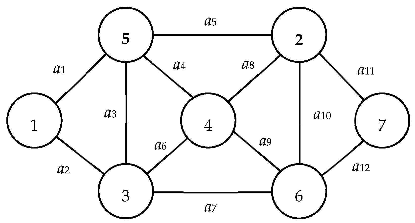
| G(V, E): | A graph with V, E, source node 1, and sink node n; for example, Figure 1 is a graph with V = {1, 2, …, 7}, E = {a1, a2, …, a12}, source node 1, and sink node 7. |
| Db: | State distribution lists the probability for each working arc; e.g., Db = {Pr(a1) = Pr(a3) = Pr(a5) = Pr(a7) = Pr(a9) = Pr(a11) = 0.96, Pr(a2) = Pr(a4) = Pr(a6) = Pr(a8) = Pr(a10) = Pr(a12) = 0.91} in Figure 1. |
| G(V, E, Db): | Binary-state network with G(V, E) and Db. For example, Figure 1 with Db = {Pr(a1) = Pr(a3) = Pr(a5) = Pr(a7) = Pr(a9) = Pr(a11) = 0.96, Pr(a2) = Pr(a4) = Pr(a6) = Pr(a8) = Pr(a10) = Pr(a12) = 0.91} is a binary-state network. |
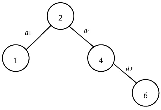
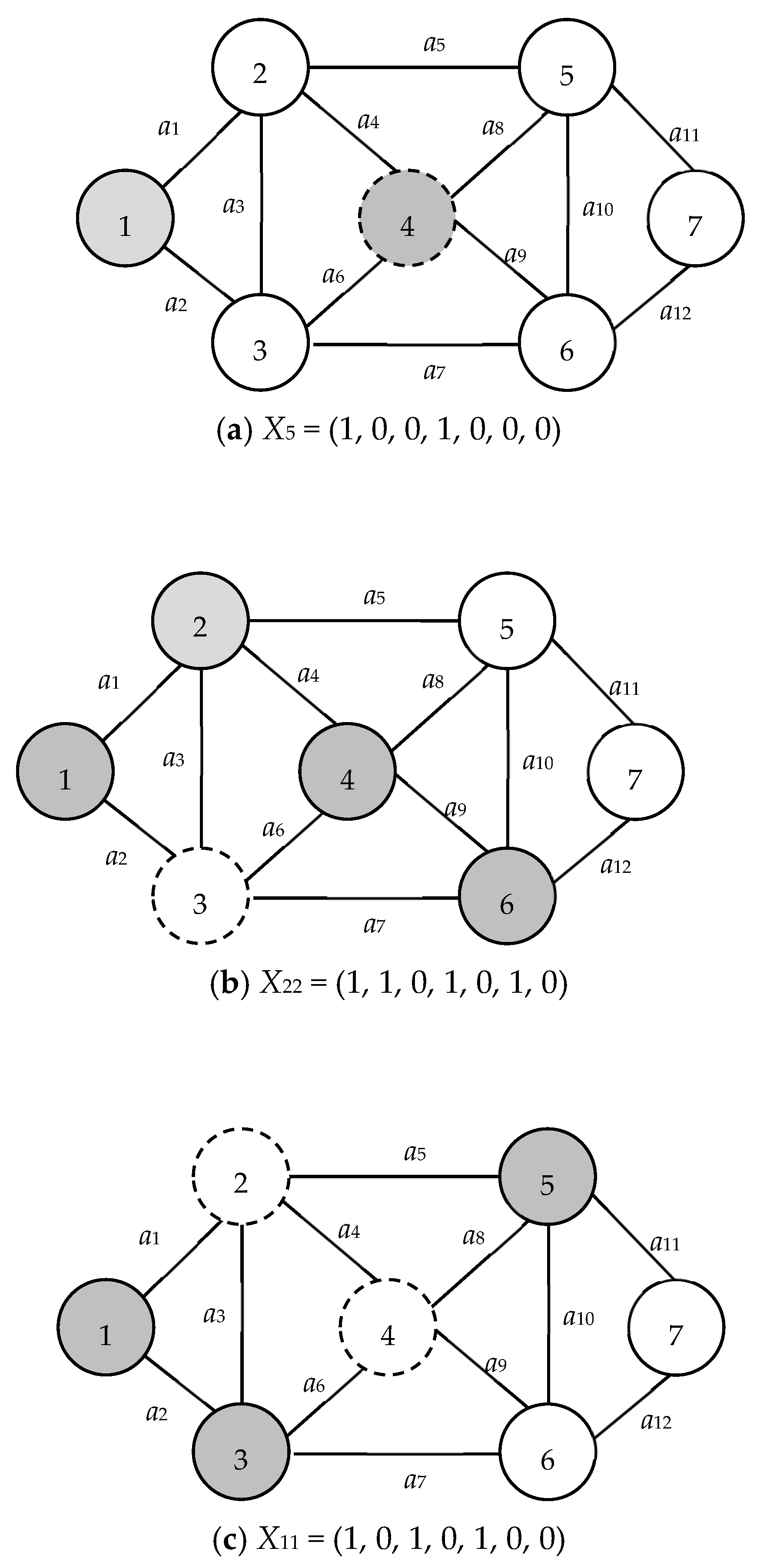
| X: | X = (X(1), X(2), …, X(|V|)) is a |V|-tuple node-based vector obtained from BAT such that its kth coordinate X(k) is represented whether node k is in the subnetwork with node 1 after the related cut. Note that X(1) = 1 and X(|V|) = 0 for all X. For example, X22 = (1, 1, 0, 1, 0, 1, 0) is the 22nd vector obtained from the BAT and denotes nodes 2, 4, and 6 are in the subnetwork with node 1 as shown in Figure 2. |
| S(X): | Node subset S(X) = {v ∊ V|X(v) = 1} ∪ {1}. For example, S(X22) = {1, 2, 4, 6} (see Figure 2) if X22 = (1, 1, 0, 1, 0, 1, 0) in Figure 1. |
| T(X): | Node subset T(X) = {v ∊ V|X(v) = 0} ∪ {n} = V − S(X). For example, T(X22) = {3, 5, 7} if X22 = (1, 1, 0, 1, 0, 1, 0) in Figure 1. |
| C(X): | Arc subset C(X) = ⌀ and {a ∊ E|for all a with one endpoint in S(X) and another one in T(X)} if X is infeasible or feasible, respectively. For example, C(X22) = ⌀ and C(X24) = {a5, a8, a10, a12} because X22 = (1, 1, 0, 1, 0, 1, 0) is infeasible, as shown in Figure 2, and X24 = (1, 1, 1, 1, 0, 1, 1) is feasible (Figure 3). |
| V(k): | Node subset V(k) = {j ∊ V|for all undirected arc a ∊ E from node k to node j ∊ V}. For example, V(2) = {1, 3, 4, 5} in Figure 1. |
| Pr(●): | Probability to have ● successfully, i.e., |
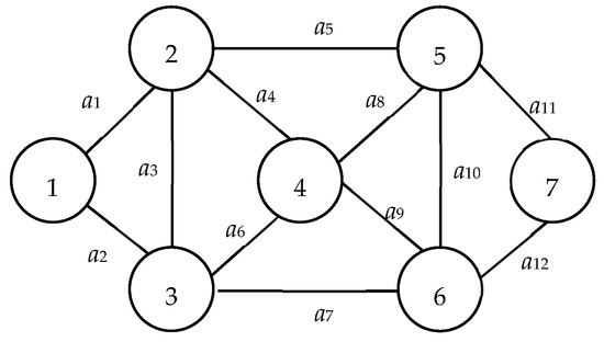
Figure 1.
Example network 1.
2.2. Assumptions
- Every individual node, denoted as v, is characterized by impeccable reliability. Furthermore, there exists at least one uncomplicated path that connects nodes 1 and n through node v.
- Every arc either operates effectively or is characterized by a failure. The probability of its occurrence operates independently, determined by a distribution grounded in empirical observations, data analysis, or rigorous testing.
- The system refrains from incorporating any loops or parallel arcs.
3. Overview of the MC, BAT, PLSA, and IET
Before delving into the proposed algorithm designed for the identification of MCs and the computation of the binary-state network reliability problem using MCs as a reference, it is pivotal to elucidate the foundational concepts underpinning the algorithm. These encompass the MC, BAT, PLSA, and IET.
3.1. MC and MC-Based Algorithms
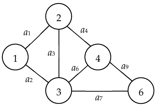
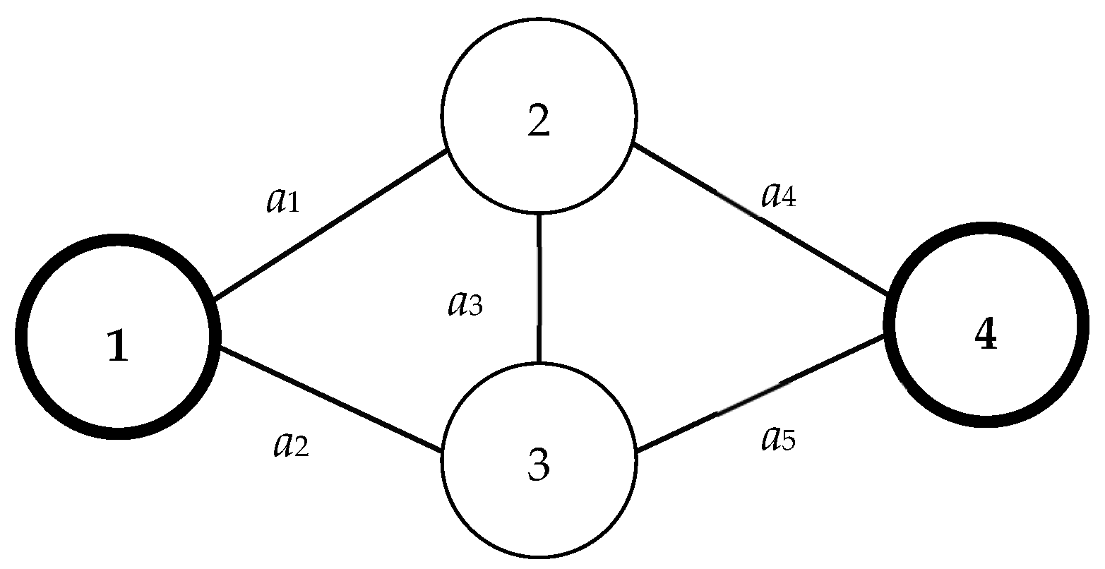
An MC, or minimal cut, is a distinct type of cut that, upon removal, bifurcates the network into two separate subnetwork nodes. This ensures that nodes 1 and n are not located within the same subnetwork. The distinction between a generic cut and an MC lies in the redundancy of arcs. Specifically, no arc within an MC is redundant; thus, the removal of any single arc from an MC would prevent it from functioning as a cut. To illustrate, consider Figure 4, which presents a comprehensive MC set, C, composed of: C1 = {a1, a2}, C2 = {a1, a3, a5}, C3 = {a2, a3, a4}, and C4 = {a4, a5}. In contrast, the arc subset C* = {a1, a2, a3} is merely a cut and not an MC. This is attributed to the arc a3 being extraneous and thus removable from C*.
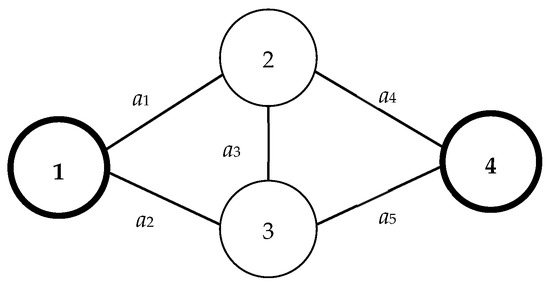
Figure 4.
Example network 2.
The quest for minimal cuts (MCs) has spawned a multitude of methods, given the critical role MCs play in addressing binary-state network reliability challenges.
Typically, the quantity of arcs is quadratic in relation to the number of nodes, rendering the node–MC algorithm more adept at efficiency when identifying all MCs compared to its arc-based counterparts. The intricacies of the BAT-integrated node–MC algorithm are detailed in Section 4.
3.2. BAT
Yeh [28] was the pioneer in developing the arc-based binary array technique (BAT), which operates based on two fundamental rules to generate every conceivable binary-state vector:
| Rule 1: | The coordinate, denoted as X(i), exhibiting the inaugural zero value undergoes a transformation to one, while X(j) is set to zero for every j < i. |
| Rule 2: | In instances where X(i) = 1 for every i, the process is terminated, signifying the identification of all vectors. |
The aforementioned BAT rules are delineated in a more structured manner via the following pseudocode, as derived from Algorithm 1 [31]:
| Algorithm 1: Arc-based BAT [31] | |
| Input: | |E|. |
| Output: | All |E|-tuple binary-state vectors. |
| STEP 0. | Assign the values: i = 1 and X = 0. |
| STEP 1. | When X(ai) is 0, set both X(ai) and i to 1, then proceed to STEP 1. |
| STEP 2. | Halt if i = |E|. |
| STEP 3. | Increase i by 1, update X to 0, and return to STEP 1. |
The BAT operates on a “you-only-look-once” (YOLO) principle. This characteristic ensures that only the vector X undergoes iterative updates within the concise arc-based BAT pseudocode, obviating the need for its preservation. Evidently, with merely four lines and a singular X, the BAT exemplifies simplicity in coding. Moreover, its efficiency in execution, frugality with memory usage, and adaptability make it an ideal choice. Consequently, BAT has found widespread applicability in diverse domains.
3.3. Layers and PLSA
Network reliability can be conceptualized as the probability that a network remains successfully connected under predefined conditions. Consequently, within the realm of network reliability challenges, there is an imperative to validate the connectivity of the resultant state vectors, independent of whether they are derived from MC- or MP-based algorithms. In pursuit of an efficient connectivity verification, the PLSA was initially introduced in [28].
Tracing its lineage, the PLSA is a progeny of the layered-search algorithm (LSA) [30]. LSA is distinctive for its formation of numerous non-overlapping node subsets: L1, L2, …, Ll, where Li is the ith node subset including all nodes in the ith layer. These subsets, referred to as layers in the LSA, are generated sequentially, ensuring each node in Li shares an arc with a node in Li+1 but not with Li+j for j = 1, 2, …, (l − i). Taking node s as the solitary constituent of L1, the presence of node t in any layer distinct from L1 infers a connection between nodes 1 and n. The pseudocode for the PLSA is delineated Algorithm 2:
| Algorithm 2: PLSA [29] | |
| Input: | G(V, E) and vector X. |
| Output: | Whether nodes 1 and n is connected in G(X). |
| STEP 0. | Assign the values: i = 2 and L1 = {1}. |
| STEP 1. | Let Li = { v ∊ V|v ∉ (L1 ∪ L2 ∪ … ∪ Li−1) and u ∊ Li−1 are two endpoints of a ∊ E }. |
| STEP 2. | Halt and X is disconnected if Li = ⌀. |
| STEP 3. | Halt and X is connected if n ∊ ⌀. |
| STEP 4. | Increase i by one and return to STEP 1. |
The time complexity associated with the PLSA stands at O(|V|). This efficiency arises from the fact that each node is incorporated into a layer at most once. Consequently, the PLSA stands out both for its simplicity and its computational efficiency. To illustrate, referring to Figure 1, the procedure elucidating the determination of connectivity for S(X22) can be found depicted in Figure 2, where X22 = (1, 1, 0, 1, 0, 1, 0). The process from the proposed PLSA for Figure 2 is shown in Table 1.

Table 1.
Process from the proposed PLSA for Figure 2.
3.4. IET
Owing to its lucidity and pivotal functionality, the IET algorithm is frequently employed in network reliability computations, especially when all MCs are identified. The IET facilitates the calculation of binary-state network reliability, drawing from the subsequent equation delineated in [29]:
where Ik is the set of k different MPs, supp(Pk) = {X|X ≥ Xk}, Xk is the k-th 1-MP, i.e., Xk(ai) = , supp(Pk) ∩ supp(Pl) = {X|X ≥ Max(Xk, Xl) = = supp(Pk ∪ Pl).
Each constituent term situated on the right-hand side of Equation (1) represents an intersection within MC subsets and is thus designated as an IET term. The probability, as articulated by Equation (1) and framed within the context of MCs, is computed in the ensuing manner:
R#(G) = [Pr(C1) + Pr(C2) + Pr(C3) + Pr(C4)] − [Pr(C1 ∩ C2) + Pr(C1 ∩ C3) + Pr(C1 ∩ C4) + Pr(C2 ∩ C3) + Pr(C2 ∩ C4) + Pr(C3 ∩ C4)] + [Pr(C1 ∩ C2 ∩ C3) + Pr(C1 ∩ C2 ∩ C4) + Pr(C1 ∩ C3 ∩ C4) + Pr(C2 ∩ C3 ∩ C4) ] − Pr(C1 ∩ C2 ∩ C3 ∩ C4).
= Pr({a1, a2}) + Pr({a1, a3, a5}) + Pr({a2, a3, a4}) + Pr({a4, a5}) − [Pr({a1, a2, a3, a5}) + Pr({a1, a2, a3, a4}) + Pr(({a1, a2, a4, a5}) + Pr({a1, a2, a3, a4, a5}) + Pr({a1, a3, a4, a5}) + Pr({a2, a3, a4, a5})] + [Pr({a1, a2, a3, a4, a5}) + Pr({a1, a2, a3, a4, a5}) + Pr({a1, a2, a3, a4, a5}) + Pr({a1, a2, a3, a4, a5})] − Pr({a1, a2, a3, a4, a5}).
= Pr({a1, a2}) + Pr({a1, a3, a5}) + Pr({a2, a3, a4}) + Pr({a4, a5}) − [Pr({a1, a2, a3, a5}) + Pr({a1, a2, a3, a4}) + Pr(({a1, a2, a4, a5}) + Pr({a1, a2, a3, a4, a5}) + Pr({a1, a3, a4, a5}) + Pr({a2, a3, a4, a5})] + [Pr({a1, a2, a3, a4, a5}) + Pr({a1, a2, a3, a4, a5}) + Pr({a1, a2, a3, a4, a5}) + Pr({a1, a2, a3, a4, a5})] − Pr({a1, a2, a3, a4, a5}).
4. BAT-BASED NODE-BASED MC
In this section, we present a modification of the widely recognized node-based MC algorithm, tailored specifically for BAT integration. This adaptation seamlessly amalgamates the principles of MC, the MC algorithm, the PLSA, and the BAT.
4.1. Pseudocode
The node-based MC algorithm was originally implemented based on DFS. From the experiments, BAT was found to be more efficient than DFS. A BAT-based node-based MC algorithm is first proposed, and its pseudocode is Algorithm 3:
| Algorithm 3: Proposed BAT-Based Node-Based MC Algorithm [29,30,31] | |
| Input: | G(V, E), source node 1 and sink node n. |
| Output: | All MCs. |
| STEP 0. | Assign the values: X = 0, i = 1 and Ω = {{a ∊ E|a is adjacent to node 1}}. |
| STEP 1. | Reassign the values of X(i) and i to be 1 if X(i) = 0, and then proceed to STEP 4. |
| STEP 2. | Stop the process if u = |V|. |
| STEP 3. | Assign X(i) to 0, increment i by 1, and then proceed to STEP 1. |
| STEP 4. | If both G(S(X)) and G(T(X)) are connected subgraphs without isolated nodes, then let Ω = Ω ∪ {C(X)} because C(X) is an MC. Proceed to STEP 1. |
The pseudocode described primarily integrates the node-based MC algorithm within the foundational framework of BAT. Nonetheless, two salient distinctions emerge:
- The vector X transitions from being an arc-based |E|-tuple in Algorithm 1 to a node-based |V|-tuple.
- An additional STEP 4 is incorporated to identify the MC subsequent to acquiring a new iteration of X.
In terms of time complexity, the above-proposed BAT’s requirement to ascertain all |V|-tuple binary-state vectors stands at O(|V|2|V|). Implementing the PLSA in STEP 4 carries a time complexity of O(|V|) for each vector processed. Consequently, the time complexity of the proposed BAT-centric node-based MC algorithm culminates at O(|V|22|V|) when tasked with discovering all the MCs within binary-state networks.
4.2. Step-by-Step Example
We employ the binary-state network depicted in Figure 1 as an illustrative example to elucidate the sequential procedure inherent to the proposed BAT-centric node-based MC algorithm, aimed at methodically uncovering all MCs. The steps are detailed as follows:
| STEP 0. | Assign the values: X = 0, i =1 and Ω = {{a1, a2}}. |
| STEP 1. | Given that X(1) = 0, set it to 1, assign i as 1, and proceed to STEP 4. |
| STEP 4. | Given that both G(S(X)) and G(T(X)) are connected, where S(X) = {1, 2} and T(X) = {3, 4, 5, 6, 7}, C(X) is defined as an MC with C(X) = {a2, a3, a4, a5}. Consequently, let Ω be updated to Ω = Ω ∪ {C(X)}, resulting in Ω = {{a1, a2}, {a2, a3, a4, a5}}. Now, proceed to STEP 1. |
| : | |
| : | |
| STEP 1. | In X = (1, 1, 0, 0, 0, 0, 0), since X(3) = 0, we update X(3) to 1 and set i to 1. Consequently, X becomes (1, 1, 1, 0, 0, 0, 0). Now, proceed to STEP 4. |
| STEP 4. | Given that G(S(X)) is disconnected, C(X) does not qualify as an MC. Proceed to STEP 1, noting that S(X) = {1, 2, 3}. |
| : | |
| : | |
| STEP 2. | Because i = |V| = 7, halt. |
The entire procedure, along with its corresponding outcomes, are comprehensively cataloged in Table 2. Within this table, a vector X is deemed feasible if the values associated with S(X), T(X), C(X), and U(X) = T(X) ∩ {all nodes adjacent to arcs in C(X)} are enumerated.
Table 2.
All Xi and MCs obtained from the proposed node-based BAT.
5. Proposed Novel Concepts
A paramount distinction between the algorithm proposed herein and the one delineated in Section 4 lies in the recursive approach employed to authenticate the connectivity across all extracted vectors. The nuances of this methodology are expounded upon in the subsequent discourse of this section.
5.1. Renumber Nodes Based on the PLSA
Let vector X(v) = 0 for all v ≥ u. Vector X* is called the son of X if X*(v) = , and X# is an offspring of X if X << X# and X#(v) = X(v) for all v < u. For example, let X6 = (1, 1, 0, 1, 0, 0, 0). X14 = (1, 1, 0, 1, 1, 0, 0) is the son of X6 and X14 = (1, 1, 0, 1, 1, 0, 0) and X22 = (1, 1, 0, 1, 0, 1, 0) and X30 = (1, 1, 0, 1, 1, 1, 0) are the offspring of X6.
As detailed in Table 2, the vector X5 = (1, 0, 0, 1, 0, 0, 0) is characterized as infeasible. Correspondingly, all its progeny vectors—namely X13 = (1, 0, 0, 1, 1, 0, 0), X21 = (1, 0, 0, 1, 0, 1, 0), and X29 = (1, 0, 0, 1, 0, 1, 0)—which share identical values for the first four coordinates with X5, are also adjudged infeasible.
Notably, this observed pattern does not universally hold. For instance, considering the same network with the positions of nodes 2 and 5 interchanged, as depicted in Figure 5, X5 = (1, 0, 0, 1, 0, 0, 0) remains infeasible. Yet, one of its derivations, X13 = (1, 0, 0, 1, 1, 0, 0), now emerges as feasible, diverging from the scenario in Figure 1.

Figure 5.
Example network with nodes 2 and 5 swapped from their positions in Figure 1.
Consider an infeasible vector X, with coordinates X(i) = 0 for i = k + 1, k + 2, …, n − 2. If both G(S(X)) and G(T(X)) remain disconnected even after updating the coordinates to X(i) = 1 for i = k + 1, k + 2, …, n − 2, it implies that all progeny of X are inherently infeasible. Consequently, we introduce a novel method, grounded on the PLSA, to resequence the nodes. The objective is to ascertain a configuration where, given an infeasible vector, all its derivations are likewise infeasible. This strategy enables the algorithm to bypass associated infeasible derivations once the infeasibility of a parent vector is established, thus reducing the count of the vectors evaluated for feasibility.
Table 3 delineates the layers, L(i), obtained from executing STEP 1 for each i and the layer value, λ(v), associated with each node v based on the structure in Figure 1.
| Algorithm 4: PLSA-based Renumber Nodes [29] | |
| Input: | G(V, E), source node 1 and sink node n. |
| Output: | All MCs. |
| STEP 0. | Implement Algorithm 2 to find L1, L2, …, Ll and λ(v) for all nodes v ∊ V. |
| STEP 1. | Renumber nodes such that nodes i < j if nodes i and j are in LƖ and Lφ, respectively, with Ɩ ≤ φ. |
| STEP 2. | Renumber nodes in each layer such that nodes i < j if nodes λ(i) > λ(i). |
Table 3.
Example of Algorithm 4.
5.2. Recursive Concept
The recursive BAT methodology is designed to systematically produce and evaluate every conceivable binary-state vector for a specified system. This technique is predominantly employed in addressing network reliability challenges, with a specific focus on connectivity characterized by minimal paths (MPs) and minimal cuts (MCs).
In [29], the recursive BAT methodology was first presented to utilize the inclusion-exclusion principle in determining network reliability following the identification of MPs. This manuscript further refines the algorithm to seamlessly incorporate edge nodes, thereby improving the process of evaluating the feasibility of vectors stemming from previously established feasible vectors.
In the proposed recursive BAT [29], there are (|V| − 2) iterations for the problem discussed here without needing to check the states of nodes 1 and n. The ith iteration has 2(Ɩ−1) vectors, where Ɩ = nj−1 is the number of vectors in the (i − 1)th iteration for i = 2, 3, …, (|V| − 2) and the first iteration has 2 vectors. Each vector, say X, in the ith iteration with X(j) = 0 for j = (i + 1), (i + 2), …, (|V| − 2). Hence, without the loss of generality and for convenience, X generated in the ith iteration is written in i-tuple because X(j) = 0 for all j > i.
Let Xj be the jth vector generated, Xi,j be the jth vector in the ith iterative for j = 1, 2, …, 2(Ɩ−1), Ɩ = nj−1, i = 1, 2, …, (|V| − 2), X1 = X1,1 = (0), and X2 = X1,2 = (1). The following important equation is the core of recursive BAT to obtain all vectors:
Also,
S(Xi,j) = S(Xj) ∪ {(i + 2)},
U(Xi,j) = [U(Xj) − {(i+2)}] ∪ [V(i+2) − S(Xj)].
Thus, the recursive BAT can have one vector in O(1) [29], which is much faster than O(n) in the traditional BAT [28].
The application of the recursive method for Algorithm 3, visualized in Figure 1. Table 4, Table 5, Table 6, Table 7 and Table 8 showcase the resultant vectors. Specifically, both the inaugural and second iterations yield two vectors each, delineated in Table 4 and Table 5, respectively.
Table 4.
Results in the first iterative for vectors 1 and 2.
Table 5.
Results in the second iterative for vectors 3 and 4, based on vectors 1 and 2, respectively.
Table 6.
Results in the third iterative for vectors 5–8, based on that of 1–4, respectively.
Table 7.
Results in the fourth iterative for vectors 9–16, based on that of 1–8, respectively.
Table 8.
Results in the last iterative for vectors 17–32, based on that of 1–16, respectively.
It is imperative to acknowledge that within these tables both Xi,j and Xj are arrayed within a congruent row. Distinctive differences between these vectors are emphasized in bold for clarity and ease of reference.
5.3. Edge Nodes for Feasible Vectors
The functions O(|S(X)|) and O(|T(X)|) are employed to assess the connectivity of G(S(X)) and G(T(X)), respectively. Their purpose is to ascertain if C(X) qualifies as an MC for any novel vector X. Given X as a feasible binary vector of dimension (n − 2)-tuple, a novel concept named the edge node subset, denoted as U(X), has been introduced. Specifically, node t is classified as an edge node if and only if es,t is an element of E, with nodes s and t positioned in S(X) and T(X), respectively. Consequently, an edge node can be interpreted as a node residing at the periphery of MC C(X).
To elucidate with a tangible instance derived from Figure 1: X23 with a value of (1, 0, 1, 1, 0, 1, 0), U(X23) is represented by the set {2, 5}. Similarly, X24 with a value of (1, 1, 1, 1, 0, 1, 1), U(X24) is defined by the set {5}. It is pertinent to note that the corresponding MCs are C(X23) = {a4, a5, a6, a9, a12} and C(X24) = {a5, a8, a10, a12}.
Given a feasible vector X, it follows that t is an element of U(X) and τ belongs to the set difference [T(X) − U(X)]. Additionally, the components X(t) and X(τ) are both set to 0. To evaluate the feasibility of X* grounded on its antecedent vector X, we can distinguish two cases:
If there is no path linking any node within S(X) to any node in the set [T(X) − U(X)], it can be concluded that X* is infeasible. As an illustration from Figure 1, the vector X2 = (1, 1, 0, 0, 0, 0, 0) is feasible. Given that node 6 belongs to the set [T(X1) − U(X1)], the vector (1, 1, 0, 0, 0, 1, 0) is deemed infeasible.
By recognizing the edge nodes, the aforementioned rule can be executed in O(1) time to ascertain whether both S(X) and T(X) form connected subgraphs. This is considerably more efficient than the O(n) time complexity characteristic of Algorithm 3, which is premised on the PLSA.
If the graph G(U(X) − {t}) exhibits connectivity, both S(X*) and T(X*) are also connected. This implies that C(X*) is indeed an MC, given the precondition that both S(X) and T(X) are connected.
Conversely, if G(U(X) − {t}) is disconnected, C(X*) cannot be classified as an MC. Employing the PLSA, verifying the connectivity of G(U(X) − {t}) requires O(|U(X) − {t}|) << O(|T(X)|) time complexity. Notably, O(|U(X) − {t}|) is much smaller than O(|T(X)|). Therefore, the aforementioned approach presents a more efficient alternative to directly employing the PLSA for ascertaining the connectivity of T(X).
In summary, by considering the aforementioned two scenarios, the introduction of edge nodes significantly bolsters the efficiency of the PLSA.
5.4. Isolated Nodes
Edge nodes serve as a valuable metric to ascertain the feasibility or infeasibility of a vector. To further enhance our understanding and analytical capabilities, not just for a singular vector but also its derivatives, the new concept of “isolated nodes” has been introduced.
An isolated node, within the context of G(X), is defined in the following manner: Node v is deemed an isolated node if it satisfies one of two conditions:
- v is an element of S(X), but in G(S(X)) it fails to establish a path to node 1.
- Conversely, v belongs to T(X), but within G(T(X)) it is unable to connect to node n.
A pivotal observation here is that the existence of at least one isolated node in X is indicative of a disconnection either in G(S(X)) or G(T(X)). This provides a direct means to infer the connectivity status of the subsets S(X) and T(X) based on the presence or absence of isolated nodes.
In the representation provided by Figure 6, nodes with a dark shading fall within S(X), whereas those colored white are members of T(X). Nodes represented with a dashed outline are identified as isolated nodes. Within the subfigures of Figure 6:

Figure 6.
Example network 3.
These distinctions among the isolated nodes, visually differentiated in the figure, allow for a deeper understanding of the positional relevance and behavior of nodes within the context of S(X) and T(X).
Nodes have been sequenced based on the layering derived from the PLSA, as elaborated in Section 5.1. Within the framework of vector X, as illustrated in Figure 3, it is infeasible to establish a pathway from either node 1 or node n to any isolated node v. In essence, the presence of an isolated node within X in G(X) dictates that X is infeasible. The positioning of node v can be categorized as inside, outside, or future.
Furthermore, there is an inherent inability to append any nodes to S(X) in such a manner that such node is no longer isolated. As a consequence, both X and all its derivatives (offspring) are deemed infeasible. Notably, when X is externally isolated, its predecessor, denoted by X1 = (1, 0, 0, 0, 0, 0, 0), cannot be expanded to produce any new derivatives, such as (1, 0, 0, 0, 1, 0, 0) or (1, 0, 0, 0, 0, 1, 0). It is crucial to highlight that both C(X1) and X3 are retained because C(X1) qualifies as a genuine MC and X3 = (1, 0, 1, 0, 0, 0, 0) had been previously generated prior to the instantiation of X5 = (1, 0, 0, 1, 0, 0, 0).
5.5. Fathom Vectors Based on Isolated Nodes
Given a feasible vector X, assume Xi is a derivative of X such that Xi(u) = and X(vi) = 0, where λ(v) < λ(v1). Based on the insights provided in Section 5.3 and Section 5.4, the following rules can be established:
- Infeasibility of X1: Vector X1 is infeasible if node v1 is not an element of U(X).
- Inside Isolated Node Condition: X2 and its derivatives are infeasible if X2(v2) = 1 for every v in U(X) and X(u) = 0, where λ(u) < λ(v2). In this scenario, u is termed as an inside isolated node.
- Outside Isolated Node Condition: X2 and its derivatives are deemed infeasible if X2(v) = 0 for all v in the λ(v)th layer and λ(u) < λ(v2). Here, u is categorized as an outside isolated node. As an added nuance, the parent of X can be excluded from the recursive list.
- Future Isolated Node Condition: X2 and its derivatives are infeasible if X2(v2) = 1, X(u) = 0, both u and v2 are elements of U(X), u < v2, and U(X) is not connected. In this situation, u is defined as a future isolated node.
- Feasibility of X2: X2 is feasible if v2 is an element of U(X) and one of the subsequent conditions holds true:
- (1)
- v2 is an independent node.
- (2)
- v2 is a dependent node and X(u) = 1 for all nodes u that depended on v2.
These rules provide a structured approach to deduce the feasibility or infeasibility of vectors, thereby enabling a systematic understanding of the network structure. This recursive nature leads to several computational advantages:
- Efficiency in Connectivity Verification: The rules preclude the need for redundant connectivity checks for both X and all its derivatives X*, significantly reducing the computational overhead.
- Optimized Vector Generation: By establishing conditions for the infeasibility of vectors, the rules effectively minimize the unnecessary generation of vectors in the BAT, leading to a faster algorithm runtime.
- Systematic Fathoming: By incorporating these rules into the proposed algorithm, we ensure that the process will efficiently dismiss or validate not just individual vectors but entire sets of related vectors. This ensures a comprehensive, yet efficient, exploration of the solution space.
In summary, integrating these structured rules into the algorithm amplifies its efficiency, making it adept at swiftly navigating through the complexities of network structures.
6. Proposed Algorithm
In this section, we elucidate the proposed algorithm through its pseudocode, illustrate its application via a representative example, and subject it to empirical evaluation through performance testing.
6.1. Pseudocode
The following Algorithm 5 presents the pseudocode for the node-based recursive BAT algorithm we have proposed.
| Algorithm 5: Proposed Node-based Recursive BAT [31] | |
| Input: | G(V, E), source node 1 and sink node n. |
| Output: | All MCs. |
| STEP 0. | Determine V(v) and λ(v) for all v ∊ V utilizing the PLSA. Initializing the values: set i to 2, j to 1, both N and N* to 2, X1 to (0), X2 to (1), S(X1) to {1}, S(X2) to {1, 2}, U(X1) to V(1), U(X2) to the difference between V(2) and {1}, and Ω to the set containing C(X1) and C(X2). |
| STEP 1. | Let X(v) = and S(X) = S(Xj) ∪ {(i+1)} based on Equations (3) and (4). |
| STEP 2. | If G(X) contains an isolated node denoted as u, then X and its offspring are deemed infeasible. Proceed to STEP 3. If not, advance to STEP 4. |
| STEP 3. | Eliminate Xj and proceed to STEP 4 if u is an outside isolated node. |
| STEP 4. | If node (i + 1) = 3 ∊ U(Xj), let U(X) = U(Xj) ∪ V((i + 1)) − S(X), Ω = Ω ∪ {C(X)}, N = N + 1 = 3, and XN = X. |
| STEP 5. | Increase j by 1 and proceed to STEP 1 if j < N*. |
| STEP 6. | If i < (|V| − 2), let i = i + 1, j = 1, N* = N, and go to STEP 1. Otherwise, terminate the process and Ω constitutes a complete MC set. |
The ensuing pseudocode delineates the node-based recursive BAT algorithm.
STEP 0: Leverage the PLSA to compute V(v) and λ(v) for every v ∊ V. STEP 1: Building on the conceptual framework presented in the iterative BAT from [25]; this step endeavors to identify all vectors. Notably, the representation of X transitions from being an arc-based |E|-tuple vector to a node-based (|V| − 2)-tuple vector. STEPs 2-4: The connectivity of S(X) is validated, relying on the layer number and the properties introduced in Section 5.1.
The primary computational demand for the proposed algorithm stems from the identification of all feasible vectors. This possesses a time complexity of O(2k), drawing from the iterative BAT’s mechanism to pinpoint all k-tuple binary-state vectors. Evaluating the feasibility of the identified vector necessitates O(|V| − 2), as seen in STEPs 2–4. Therefore, the overall time complexity for the algorithm, especially when discerning all MCs in binary-state networks, is O((|V| − 2)2(|V|-2)), which simplifies to O((|V| − 2)2α|V|), where α = (|V| − 2)/|V| ∊ [0, 1), i.e., Algorithm 5 outperforms Algorithm 3 and other existing related algorithms in terms of efficiency.
6.2. Step-by-Step Example
Enumerating all minimal cuts (MCs) and determining the exact binary-state network reliability in terms of MCs within binary-state networks are acknowledged to be NP-hard and #P-hard challenges, as highlighted by reference [11]. Consequently, as the scale of the network increases, the computational burden escalates exponentially.
A seminal benchmark for binary-state networks is portrayed in Figure 1, which is recurrently referenced in literature [8,9,10,11,12,13,14,15]. Its moderate scale renders it particularly apt to elucidate the stages of the proposed algorithm.
| STEP 0. | Determine V(v) and λ(v) for all v ∊ V as shown in Table 4 and Table 5; let i = 2, j = 1, (|V| − 2) = 5, X1 = (0), S(X1) = {1}, U(X1) = V(1), X2 = (1), S(X2) = {1, 2}, U(X2) = V(2) − {1} = {3, 4, 5}, N = N* = 2, and Ω = {C(X1), C(X2)} = {{a1, a2}, {a2, a3, a4, a5}}. |
| STEP 1. | Let X(v) = , i.e., X = (0, 1), and S(X) = S(Xj) ∪ {(i + 1)} = {1, 3}. |
| STEP 2. | Because G(X) has no isolated nodes, proceed to STEP 4. |
| STEP 4. | Because node (i + 1) = 3 ∊ U(Xj), X is feasible and let U(X) = U(Xj) ∪ V((i + 1)) − S(X) = {2, 3} ∪ {1, 2, 4, 6} − {1, 3} = {2, 4, 6}, Ω = Ω ∪ {C(X)} = {{a1, a2}, {a2, a3, a4, a5}, {a1, a3, a6, a7}}, N = N + 1 = 3, and XN = X. |
| STEP 5. | Because j = 1 < N* = 2, let j = j + 1 = 2, and go to STEP 1. |
| STEP 1. | Let X(v) = , i.e., X = (1, 1), and S(X) = S(X2) ∪ {(2 + 1)} = {1, 2, 3}. |
| STEP 2. | Because there are no isolated nodes in G(X), go to STEP 4. |
| STEP 4. | Because node (i + 1) = 3 ∊ U(Xj), let U(X) = U(X2) ∪ V(3) − S(X) = {4, 5, 6}, Ω = Ω ∪ {C(X)} = { {a1, a2}, {a2, a3, a4, a5}, {a1, a3, a6, a7}, {a4, a5, a6, a7} }, N = N + 1 = 4, and XN = X4 = X. |
| STEP 5. | Because j = N* = 2, go to STEP 6. |
| STEP 6. | Because i = 2 < (|V| − 2) = 5, let i = i + 1 = 3, j = 1, N* = N = 4, and go to STEP 1. |
| STEP 1. | Let X(v) = , i.e., X = (0, 0, 1), and S(X) = S(Xj) ∪ {(i + 1)} = {1, 4}. |
| STEP 2. | Because node 4 is isolated, X and its offspring are all infeasible and go to STEP 3. |
| STEP 3. | Because node 4 is isolated outside, remove X1 and go to STEP 5. |
| STEP 5. | Because j = 1 < N* = 4, let j = j + 1 = 2 and go to STEP 1. |
| : | |
| Assume that i = 5, j = 12, N* = 10, and N = 4. | |
| STEP 1. | Let X(v) = , i.e., X = (1, 1, 1, 1, 1), and S(X) = S(Xj) ∪ {(i + 1)} = {1, 2, 3, 4, 5, 6}. |
| STEP 2. | Because there are no isolated nodes in G(X), go to STEP 4. |
| STEP 4. | Because node (i + 1) = 6 ∊ U(Xj) is connected, let U(X) = U(X2) ∪ V(3) − S(X) = {7}, Ω = Ω ∪ {C(X)}, N = N + 1 = 5, XN = X, and go to STEP 5. |
| STEP 5. | Because j = N* = 12, go to STEP 6. |
| STEP 6. | Because i = (|V| − 2) = 5, halt and all MCs are found in Ω = {{a1, a2}, {a2, a3, a4, a5}, {a1, a3, a6, a7}, {a4, a5, a6, a7}, {a2, a3, a5, a6, a8, a9}, {a1, a3, a4, a7, a8, a9}, {a5, a7, a8, a9}, {a2, a3, a4, a8, a10, a11}, {a4, a6, a7, a8, a10, a11}, {a2, a3, a6, a9, a10, a11}, {a7, a9, a10, a11}, {a1, a3, a6, a9, a10, a12}, {a4, a6, a7, a8, a10, a11}, {a4, a5, a6, a9, a12}, {a5, a8, a10, a12}, {a11, a12}}. |
Following the implementation of the node-based recursive BAT algorithm, comprehensive results are presented in Table 4 and Table 5. These tables offer insights into the algorithm’s performance, especially in context with the benchmark binary-state network from Figure 1. It is essential to review these outcomes to grasp the algorithm’s proficiency in identifying MCs.
6.3. Computation Experiments
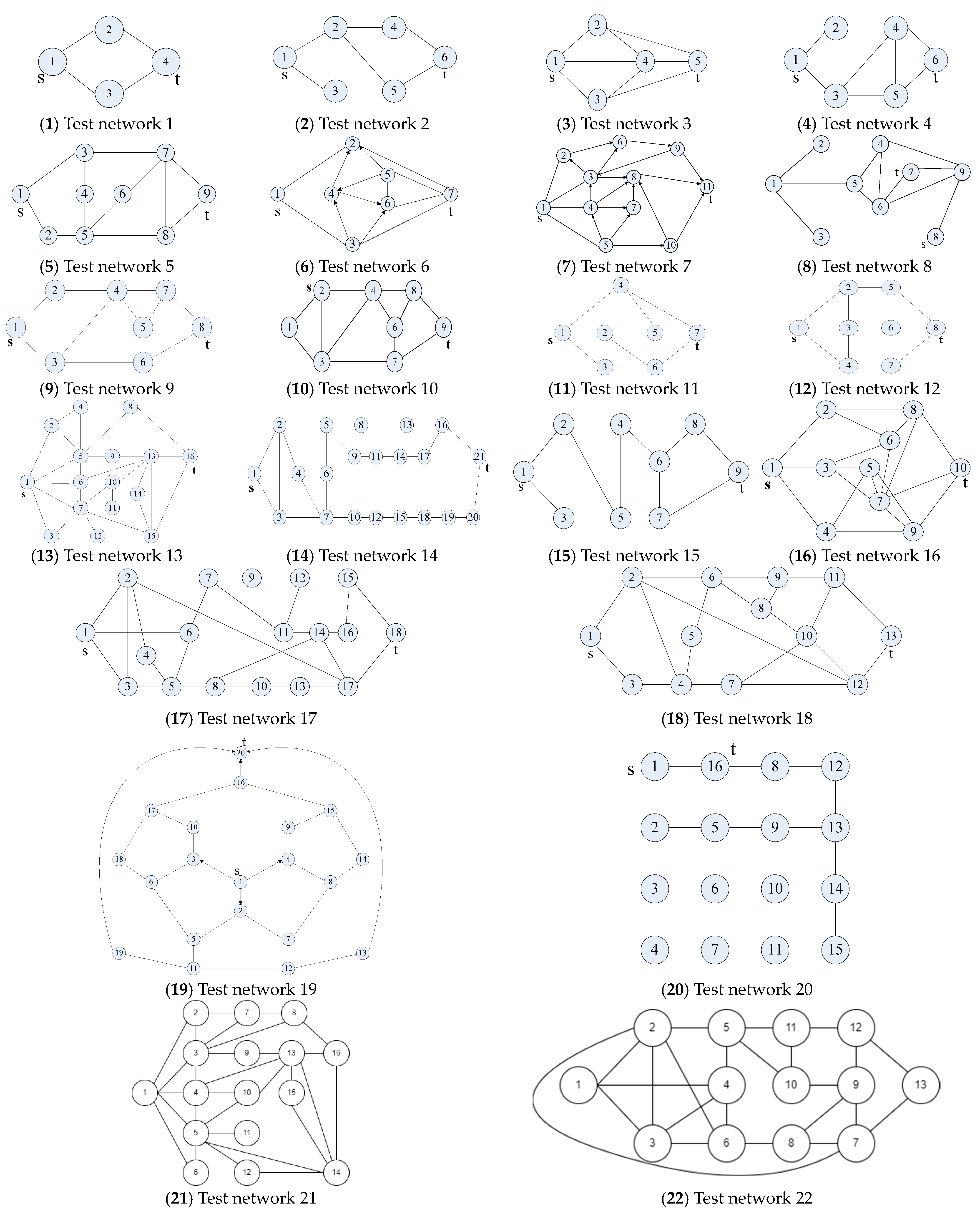
To authenticate the proficiency and efficacy of our algorithm, we subjected it to rigorous testing on well-established benchmark networks. Accordingly, we selected 20 quintessential binary-state benchmark networks, showcased in Figure 7(1–20) [11,12,13,14,15,16,17,18,19,20,21,22,23,24,25,26,27,28,29], to serve as our experimental subjects. It is imperative to mention that the node numbering sequence has been rearranged in accordance with the guidelines laid out in Section 5.1. For instance, the representations in Figure 7(13) and Figure 7(18) were remodeled as Figure 7(21) and Figure 7(22), respectively.
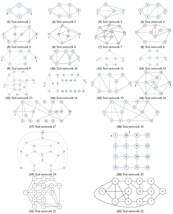
Figure 7.
Test networks.
Note that the order of node numbers is renumbered based on Section 5.1, e.g., Figure 7(13) and Figure 7(18) are redrawn to Figure 7(21) and Figure 7(22), respectively.
To critically assess the proposed algorithm’s performance, we benchmarked it against the leading node-based algorithm, adapted for BAT as elucidated in Section 4. To ensure an equitable evaluation, both algorithms were implemented using DEV C++ 5.11, operating on a 64-bit Windows 10 environment powered by an Intel Core i7-6650U processor clocked at 2.20 GHz to 2.21 GHz coupled with 32 GB of RAM. Additionally, for all tested networks, we set Pr(a) to 0.9 for every arc a.
The comparative results are tabulated in Table 9. Superior performance metrics, whether from our proposed method or the reference node-based MC algorithm, are highlighted in bold. In this context, “TNBA” signifies the quantity of vectors and the associated computation time needed by the renowned node-based algorithm, whereas “TRBAT” represents the equivalent metrics for our proposed methodology. As illustrated in Table 9, the number of derived MCs experiences an exponential increase concerning the number of nodes, “n”. This trend is consistent with the inherent characteristics of NP-hard and #P-hard challenges. Notably, both the TNBA and TRBAT are zero for “m” values less than 21. Consequently, these two algorithms prove to be efficient in solving small-scale problems. However, for “m” values greater than 21, the proposed algorithm outperforms the other one in terms of the TNBA and TRBAT values. These results demonstrate that the proposed algorithm is more suitable for larger problems.
Table 9.
Comparison of results.
As depicted in Table 9, the count of derived MCs exhibits an exponential surge relative to the number of nodes, n. This trend aligns with the inherent attributes of NP-hard and #P-hard challenges.
For more diminutive datasets, specifically those represented in Figure 7(1–12), both algorithms showcase comparable efficiencies, completing computations within 0.001 s.
A comprehensive analysis of the data from Table 10 further underscores the salient features and advantages of our approach. Specifically, the strategic reordering of node numbers, coupled with the isolated nodes concept, drastically diminishes the prevalence of infeasible vectors. Concurrently, the integration of edge nodes accelerates the feasibility verification process for vectors. Finally, the recursive algorithm framework ensures a more efficient vector generation process.
Table 10.
Comparison of the proposed algorithm and the one proposed in [19].
The empirical results delineated above align seamlessly with the comparative analysis of time complexities drawn between our proposed algorithm and the prominent MC algorithm. This congruence not only reaffirms the theoretical underpinnings but also accentuates the superiority of our algorithm over the MC methodology previously documented in [29].
7. Conclusions
Network reliability stands as a pivotal metric encapsulating the operational probability of contemporary networks. It is noteworthy that the reliability evaluations bearing real-world constraints, termed conditional network reliability, offer more pragmatic insights than their unconditional counterparts. Central to the computation of conditional network reliability is the necessity to delineate MCs and MPs.
Addressing this exigency, the present work pivots on the enhancement of the canonical binary addition tree (BAT) through the introduction of a recursive paradigm. Our innovation lies in crafting a recursive node-based BAT tailored explicitly for elucidating MCs in conditional network reliability scenarios.
Our proposed methodology distinguishes itself on multiple fronts:
- It pioneers a recursive approach within the realm of BAT algorithms aimed at MC extraction.
- The algorithm melds the agility of recursive BAT—enabling O(1) vector generation—with a strategic node renumbering scheme. This amalgamation aids in the early identification and pruning of infeasible vectors and their progeny, courtesy of the isolated node concept.
- The novel introduction of “edge nodes” further trims the computational overheads associated with feasibility verification of vectors.
Subjecting our algorithm to rigorous empirical scrutiny, we benchmarked it against the gold-standard node-based MC algorithm across 20 binary-state networks. The corroboration from both time complexity analyses and practical experiments unequivocally underscored the superiority of our recursive node-based BAT.
Paving the way forward, our ambitions extend towards stress-testing the proposed algorithm against more sizable benchmark networks. An intriguing avenue of future exploration also encompasses the algorithm’s extrapolation towards identifying d-MCs in multistate flow network (MFN) contexts.
Furthermore, to show the efficiency of the proposed method, we plan to compare it with more algorithms in the future. Additionally, further studies are planned to investigate how our model improves 4G/5G communications.
Author Contributions
Conceptualization, W.-C.Y.; methodology, W.-C.Y.; software, W.-C.Y. and G.Y.; validation, W.-C.Y.; formal analysis, W.-C.Y. and G.Y.; investigation, W.-C.Y., G.Y. and C.-L.H.; resources, W.-C.Y., G.Y. and C.-L.H.; data curation, W.-C.Y., G.Y. and C.-L.H.; writing—original draft preparation, W.-C.Y., G.Y. and C.-L.H.; writing—review and editing, W.-C.Y.; visualization, W.-C.Y.; supervision, W.-C.Y.; project administration, W.-C.Y.; funding acquisition, W.-C.Y. All authors have read and agreed to the published version of the manuscript.
Funding
This research was supported in part by the National Science and Technology Council, R.O.C., under grants MOST 107-2221-E-007-072-MY3 and MOST 110-2221-E-007-107-MY3 and NSTC 112-2221-E-007-086.
Data Availability Statement
Data is unavailability because it is a simulated experiment in this paper.
Conflicts of Interest
The authors declare no conflicts of interest.
Acronyms
| MC | Minimal cut |
| MP | Minimal path |
| DFS | depth-first search |
| IET | Inclusion–exclusion technology |
| BAT | Binary-addition-tree algorithm [28] |
| PLSA | Path-based layered-search algorithm |
Nomenclature
| Reliability | This denotes the probabilistic connection between nodes 1 and n. |
| Cut | A subset of arcs; when removed, it divides the entire graph or network into two separated subgraphs. |
| MC | A distinctive cut between nodes 1 and n that lacks any superfluous arc; its excision does not affect other MCs. In Figure 1, while {a4, a5, a6, a7} exemplifies an MC, {a4, a5, a6} represents neither a cut nor an MC. Conversely, {a2, a4, a5, a6, a7} manifests as a cut, but the arc a2 renders it redundant, thus, not qualifying it as an MC. |
| MP | A simple path transitioning from node 1 to n, devoid of any redundant arc. Illustrated in Figure 1, {a2, a7, a12} is an MP, whereas {a2, a7} does not constitute a path or an MP. However, {a1, a2, a7, a12} stands as an MP but includes the superfluous arc a1. |
| Isolated node | Within the context of X, a node v is deemed isolated if there exists no pathway from node 1 to node v or from node v to node n in the graphs G(S(X)) and G(T(X)), respectively. A case in point from Figure 1: node 3, within X22 = (1, 1, 0, 1, 0, 1, 0), is isolated since it belongs to T(X22) but lacks connectivity to node 7 in G(T(X22)). |
| Edge node | In the context of X, a node in U(X) = T(X) ∩ {all nodes adjacent to arcs in C(X)} receives the designation of an “edge node” if it is encapsulated within U(X). Drawing from Figure 1, nodes 5 and 7 both qualify as edge nodes in the set X24 = (1, 1, 1, 1, 0, 1, 1). |
| Feasible/Infeasible Vector | A vector, X, predicated on nodes, is termed “feasible” if C(X) corresponds to an MC and no isolated nodes exist within X. An instance from Figure 1 can be discerned in vectors X22 = (1, 1, 0, 1, 0, 1, 0) and X24 = (1, 1, 1, 1, 0, 1, 1). The former is infeasible due to the presence of an isolated node, node 3, whereas the latter is feasible owing to the absence of isolated nodes. |
References
- Niu, Y.F. Performance measure of a multi-state flow network under reliability and maintenance cost considerations. Reliab. Eng. Syst. Saf. 2021, 215, 107822. [Google Scholar] [CrossRef]
- Wang, W.C.; Zhang, Y.; Li, Y.X.; Hu, Q.; Liu, C.; Liu, C. Vulnerability analysis method based on risk assessment for gas transmission capabilities of natural gas pipeline networks. Reliab. Eng. Syst. Saf. 2022, 218, 108150. [Google Scholar] [CrossRef]
- Ma, G.; Huang, Y.; Li, J. Bayesian Network Analysis of Explosion Events at Petrol Stations. In Risk Analysis of Vapour Cloud Explosions for Oil and Gas Facilities; Springer: Singapore, 2019; pp. 191–217. [Google Scholar]
- Honqqum, L.; Xianlin, H.; Gao, X.Z.; Xiaojun, B.; Hang, Y. Stability analysis of the simplest Takagi-Sugeno fuzzy control system using circle criterion. J. Syst. Eng. Electron. 2007, 18, 311–319. [Google Scholar] [CrossRef]
- He, R.; Deng, J.; Lai, L.L. Reliability evaluation of communication-constrained protection systems using stochastic-flow network models. IEEE Trans. Smart Grid 2017, 9, 2371–2381. [Google Scholar]
- Aven, T. Availability evaluation of oil/gas production and transportation systems. Reliab. Eng. 1987, 18, 35–44. [Google Scholar] [CrossRef]
- Kakadia, D.; Ramirez-Marquez, J.E. Quantitative approaches for optimization of user experience based on network resilience for wireless service provider networks. Reliab. Eng. Syst. Saf. 2020, 193, 106606. [Google Scholar] [CrossRef]
- Yeh, W.C. A simple algorithm for evaluating the k-out-of-n network reliability. Reliab. Eng. Syst. Saf. 2004, 83, 93–101. [Google Scholar] [CrossRef]
- Yang, Y.; Wang, S.; Xu, W.; Wei, K. Reliability evaluation of wireless multimedia sensor networks based on instantaneous availability. Int. J. Distrib. Sens. Netw. 2018, 14, 1550147718810692. [Google Scholar] [CrossRef]
- Gongora-Svartzman, G.; Ramirez-Marquez, J.E. Social cohesion: Mitigating societal risk in case studies of digital media in Hurricanes Harvey, Irma, and Maria. Risk Anal. 2022, 42, 1686–1703. [Google Scholar] [CrossRef]
- Colbourn, C.J. The Combinatorics of Network Reliability; Oxford University Press, Inc.: New York, NY, USA, 1987. [Google Scholar]
- Shier, D.R. Network Reliability and Algebraic Structures; Clarendon Press: New York, NY, USA, 1991. [Google Scholar]
- Levitin, G. The Universal Generating Function in Reliability Analysis and Optimization; Springer: Berlin/Heidelberg, Germany, 2005. [Google Scholar]
- Pandey, M.; Zuo, M.J.; Moghaddass, R.; Tiwari, M.K. Selective maintenance for binary systems under imperfect repair. Reliab. Eng. Syst. Saf. 2013, 113, 42–51. [Google Scholar] [CrossRef]
- Ramirez-Marquez, J.E. Approximation of minimal cut sets for a flow network via evolutionary optimization and data mining techniques. Int. J. Perform Abil. Eng. 2011, 7, 21. [Google Scholar]
- Forghani-elahabad, M.; Kagan, N. Reliability evaluation of a stochastic-flow network in terms of minimal paths with budget constraint. IISE Trans. 2019, 51, 547–558. [Google Scholar] [CrossRef]
- Wang, C.; Xing, L.; Levitin, G. Reliability analysis of multi-trigger binary systems subject to competing failures. Reliab. Eng. Syst. Saf. 2013, 111, 9–17. [Google Scholar] [CrossRef]
- Larsen, E.M.; Ding, Y.; Li, Y.F.; Zio, E. Definitions of generalized multi-performance weighted multi-state K-out-of-n system and its reliability evaluations. Reliab. Eng. Syst. Saf. 2020, 199, 105876. [Google Scholar] [CrossRef]
- Moghaddass, R.; Zuo, M.J. An integrated framework for online diagnostic and prognostic health monitoring using a multistate deterioration process. Reliab. Eng. Syst. Saf. 2014, 124, 92–104. [Google Scholar] [CrossRef]
- Levitin, G. A universal generating function approach for the analysis of multi-state systems with dependent elements. Reliab. Eng. Syst. Saf. 2004, 84, 285–292. [Google Scholar] [CrossRef]
- Niu, Y.F.; Song, Y.F.; Xu, X.Z. Budget optimization for a multi-distribution multi-state logistics network with reliability consideration. Qual. Technol. Quant. Manag. 2023, 20, 528–544. [Google Scholar] [CrossRef]
- Levitin, G.; Gertsbakh, I.; Shpungin, Y. Evaluating the damage associated with intentional supply deprivation in multi-commodity network. Reliab. Eng. Syst. Saf. 2013, 119, 11–17. [Google Scholar] [CrossRef]
- Lin, S.; Jia, L.; Zhang, H.; Zhang, P. Reliability of high-speed electric multiple units in terms of the expanded multi-state flow network. Reliab. Eng. Syst. Saf. 2022, 225, 108608. [Google Scholar] [CrossRef]
- Zhou, J.; Coit, D.W.; Felder, F.A.; Wang, D. Resiliency-based restoration optimization for dependent network systems against cascading failures. Reliab. Eng. Syst. Saf. 2021, 207, 107383. [Google Scholar] [CrossRef]
- Khan, A.; Bonchi, F.; Gullo, F.; Nufer, A. Conditional reliability in uncertain graphs. IEEE Trans. Knowl. Data Eng. 2018, 30, 2078–2092. [Google Scholar] [CrossRef]
- Yeh, W.C. Search for MC in modified networks. Comput. Oper. Res. 2001, 28, 177–184. [Google Scholar] [CrossRef]
- Zuo, M.J.; Tian, Z.; Huang, H.Z. An efficient method for reliability evaluation of multistate networks given all minimal path vectors. IIE Trans. 2007, 39, 811–817. [Google Scholar] [CrossRef]
- Yeh, W.C. Novel Binary-Addition Tree Algorithm (BAT) for Binary-State Network Reliability Problem. Reliab. Eng. Syst. Saf. 2020, 208, 107448. [Google Scholar] [CrossRef]
- Yeh, W.C. Novel Recursive Inclusion-Exclusion Technology Based on BAT and MPs for Heterogeneous-Arc Binary-State Network Reliability Problems. Reliab. Eng. Syst. Saf. 2023, 231, 107917. [Google Scholar] [CrossRef]
- Yeh, W.C. A revised layered-network algorithm to search for all d-minpaths of a limited-flow acyclic network. IEEE Trans. Reliab. 1998, 47, 436–442. [Google Scholar]
- Available online: https://drive.google.com/file/d/1cMkbIXqI2QlPu70oR42EgLxMMwEM_REz/view (accessed on 11 January 2023).


Disclaimer/Publisher’s Note: The statements, opinions and data contained in all publications are solely those of the individual author(s) and contributor(s) and not of MDPI and/or the editor(s). MDPI and/or the editor(s) disclaim responsibility for any injury to people or property resulting from any ideas, methods, instructions or products referred to in the content. |
© 2024 by the authors. Licensee MDPI, Basel, Switzerland. This article is an open access article distributed under the terms and conditions of the Creative Commons Attribution (CC BY) license (https://creativecommons.org/licenses/by/4.0/).