Abstract
With the powerful discriminative capabilities of convolutional neural networks, change detection has achieved significant success. However, current methods either ignore the spatiotemporal dependencies between dual-temporal images or suffer from decreased accuracy due to registration errors. Addressing these challenges, this paper proposes a method for remote sensing image change detection based on the cross-mixing attention network. To minimize the impact of registration errors on change detection results, a feature alignment module (FAM) is specifically developed in this study. The FAM performs spatial transformations on dual-temporal feature maps, achieving the precise spatial alignment of feature pairs and reducing false positive rates in change detection. Additionally, to fully exploit the spatiotemporal relationships between dual-temporal images, a cross-mixing attention module (CMAM) is utilized to extract global channel information, enhancing feature selection capabilities. Furthermore, attentional maps are created to guide the up-sampling process, optimizing feature information. Comprehensive experiments conducted on the LEVIR-CD and SYSU-CD change detection datasets demonstrate that the proposed model achieves F1 scores of 91.06% and 81.88%, respectively, outperforming other comparative models. In conclusion, the proposed model maintains good performance on two datasets and, thus, has good applicability in various change detection tasks.
1. Introduction
Remote sensing image change detection is the process of comparing dual-temporal remote sensing images of an identical geographic region captured at different time points to detect changes in the characteristics of the area [1]. With the continuous development of remote sensing technology, the acquisition of high-resolution remote sensing images has become increasingly easy, and the availability and quality of remote sensing image data have been greatly improved, further exploring the value of remote sensing images [2,3,4]. Affected by natural geographic processes and human activities, global land cover continues to undergo rapid changes, which may have profound impacts on the Earth’s environment. Change detection is an important means of comprehensive monitoring and recording of land cover changes [5,6,7,8,9]. At present, change detection has been widely applied in various fields, including changes in land use [10], urban transformations [11], responses to natural disasters [12], and forest administration [13]. Traditional change detection methods primarily emphasize the texture, shape, and spectral aspects of remote sensing images, while ignoring contextual semantic information. For instance, Celik et al. [14] used K-means clustering and principal component analysis (PCA) to discriminate between changed and unchanged pixels in remote sensing images. Jia et al. [15] enhanced the differencing method for vegetation characteristics and used the near-infrared channel to calculate normalized vegetation indices (NVIs) that are capable of detecting small changes in vegetation. Wang et al. [16] employed a detection technique utilizing double-threshold exponential entropy to calculate the optimal threshold and improve detection performance. However, the target area of remote sensing images has diverse structures and contains rich spectral information, yet traditional methods cannot effectively solve the problems of multi-category, multi-scale, and multi-level feature extraction or information fusion.
With the advancement and widespread adoption of deep learning and computer hardware, the application of convolutional neural networks (CNNs) [17,18] has been extensively embraced across various fields [19,20], fostering significant advancements in change detection technology [20]. CNNs automatically extract abundant spatial and semantic information from remote sensing images [21,22]. Consequently, some scholars have applied them to remote sensing image change detection tasks, achieving commendable results [23]. Daudt et al. [24] proposed three distinct end-to-end full convolutional neural network structures [25] for various methods of image feature extraction and fusion. They introduced Siamese networks [26] and skip connections [27] to collect features from dual-temporal images using shared weights and subsequently compared these features to detect change regions. Peng et al. [28] optimized the edge details of change regions by establishing dense connections between the encoder and decoder, effectively leveraging detailed low-level features. However, these networks produce considerable redundant information when fusing shallow and deep features, leading to false detection in the results.
This issue can be effectively mitigated by introducing an attention mechanism to emphasize crucial features in the image [29,30]. Chen et al. [31] improved the model’s performance by capturing long-range dependencies and acquiring more discriminative features through a dual attention mechanism. Shi et al. [32] enhanced model performance by utilizing the CBAM [33] attention mechanism to weigh feature map channels and optimize the semantic information of change regions. Despite enhancing the completeness of prediction results through the attention mechanism, these networks fail to address the spatial and temporal correlations between dual-temporal remote sensing images. Chen et al. [34] and Zhang et al. [35] utilized the attention mechanism across varying scales to capture spatial and temporal relationships between dual-temporal images, generating improved feature representations that effectively mitigate the pseudo-variation phenomena arising from illumination differences and similar factors. Although the use of attention mechanisms at different scales enhances the connection between temporal and spatial information, these networks adopt ordinary and non-learnable up-sampling methods, which can lead to the distortion of the predicted graph.
Currently, many excellent network structures are used for semantic segmentation tasks. For example, Chen et al. [36] used a feature pyramid to fuse feature maps at different levels, which captured multi-scale information and introduced dilated convolution to increase the receptive field. Sun et al. [37] captured more image details while maintaining high-resolution characteristics by establishing a multi-level feature map. The pyramid pooling module proposed by Zhao et al. [38] can aggregate contextual information from different regions, thereby improving the ability to obtain global information. Change detection can be seen as a binary classification problem (changed and unchanged), so it is natural to introduce excellent semantic segmentation models in change detection tasks. We can obtain the pixel range of specific targets (such as farmland, buildings, ships, etc.) through semantic segmentation. After achieving the pixel-level classification of the image content, we can then perform change detection on specific categories in the image [39,40].
Nonetheless, conventional CNN-based methods often lack the capacity to construct inter-pixel dependencies, prompting the introduction of attention mechanisms in change detection. Change detection typically employs a Siamese network framework, applying the attention mechanism separately to two images, yet it inadequately considers the connections between temporal and spatial domain features in these images. Hence, the proposed solution is the cross-mixing attention network. Initially, this network stacks dual-temporal feature maps, processed using the feature alignment module by channels. It subsequently fully fuses the dual-temporal image features via the convolution block. Finally, it routes the fused feature maps through the attention header, leveraging spatial and temporal information to establish the cross-mixing attention weight map. Utilizing weight maps to guide up-sampling not only balances global feature relationships but also compensates for the non-learnable shortcomings of conventional up-sampling methods.
The main contributions of this paper are as follows:
- (1)
- The feature alignment module is designed to resample feature maps to obtain aligned feature maps and alleviate the problem of detection accuracy degradation due to alignment error.
- (2)
- The cross-mixing attention module is designed to better utilize the spatiotemporal information between dual-temporal remote sensing images and generate the attention weight map.
- (3)
- The ordinary up-sampling method is parameterless and unlearnable; in this paper, the attention weight map is used to guide the up-sampling, optimize the global feature information, and generate a more complete change prediction map. Experimental verification confirms that the proposed network enhances the change detection performance.
2. The Proposed Method
2.1. Overall Network Structure
Figure 1 illustrates the overall architecture of the cross-mixing attention network. This network takes three channels of dual-temporal remote sensing images as input and generates a single channel for change prediction maps. Dual-temporal images are processed through a dual-branch weight-sharing encoder, utilizing EfficientNetB4 [41] for feature extraction in each branch. Extracted dual-temporal feature maps from each layer are fed into the feature alignment module (FAM), where pixel resampling corrects the feature maps, alleviating the misdetections caused by alignment errors. These corrected feature map channels are merged through the cross-mixing attention module (CMAM), employing MLP to optimize global channel-related information in the feature map and resulting in attention map generation. During decoding, the attention map guides the up-sampling process, compensating for spatial detail loss in deep features and enhancing the information within different feature maps. Finally, the difference feature map, restored to its original size, is processed by the per-pixel classifier to derive the ultimate change prediction map.
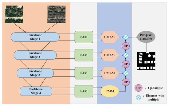
Figure 1.
Proposed method’s flow chart.
2.2. Feature Alignment Module
Remote sensing image change detection aims to identify the disparities between dual-temporal images. Alignment errors arise when aligning dual-temporal remote sensing images, influenced by factors such as imaging time, illumination, and shooting angle. These errors can obscure the target area boundary during change detection, making pseudo-change elimination challenging and ultimately impacting detection accuracy. Figure 2 illustrates the distinct differences in brightness, contrast, and spatial edges within the target area of the two images. Failure to address these differences in subsequent steps could lead to false detections along the boundaries of unchanged target regions.
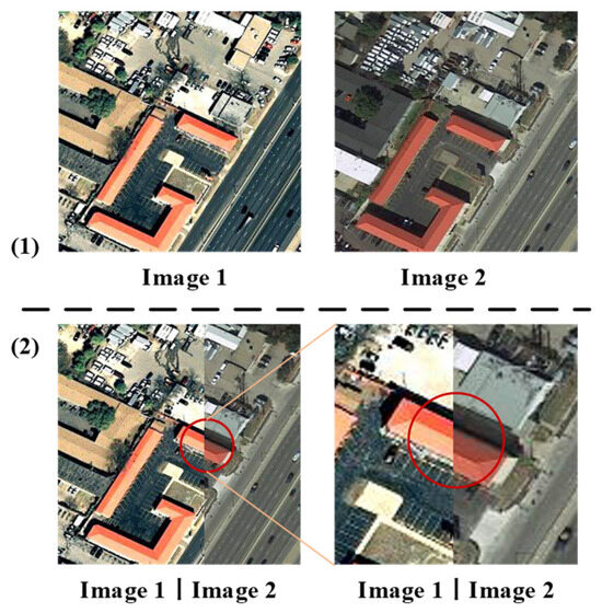
Figure 2.
(1) Dual-temporal remote sensing images; (2) misregistration errors diagram. (Red circles indicate zooming in on details for a clearer view).
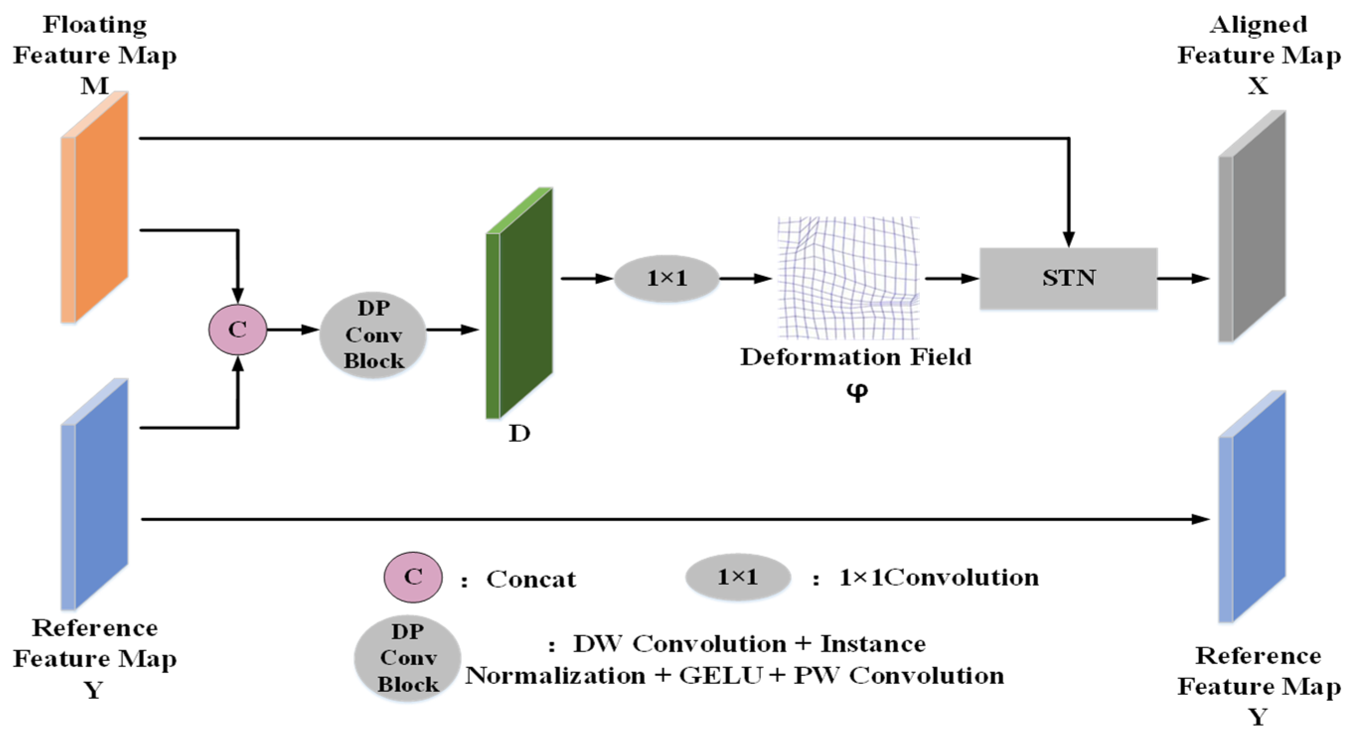
The proposed approach for mitigating the alignment error’s impact on detection accuracy involves the feature alignment module, as depicted in Figure 3. The feature map at time T1 represents the floating feature map M, while the feature map at time T2 serves as the reference feature map Y. The feature alignment module takes the floating feature map M (at time T1) and the reference feature map Y (at time T2) as inputs. Initially, it calculates the deformation field φ based on M and Y. Subsequently, it resamples the floating feature map M using spatial transformation networks (STNs) [42], resulting in the aligned feature map X. Ultimately, it outputs both the aligned feature map X and the reference feature map Y, effectively minimizing alignment error influences on change detection.
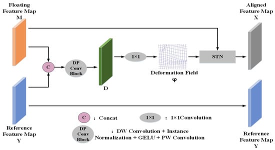
Figure 3.
Structure of feature alignment module.
As illustrated in Figure 3, the floating feature map and the reference feature map are the first channel concatenate, and the concatenate feature map is subjected to a DP convolution block operation to effectively extract the feature information of the input feature image pairs to obtain the feature map as shown in Expression (1):
where DP denotes a DP convolution block operation wherein the DP convolution block comprises the following steps:
Initially, the DWConv [43] convolutional operation extracts channel-specific feature information from the spliced feature map. Subsequently, a PWConv [43] convolutional operation captures diverse channel-specific information at identical spatial locations. Following this, InstanceNorm normalization scales the feature map values within the range of [−1, 1]. Finally, the GELU activation function introduces nonlinearity, optimizing the network’s forward propagation.
To maintain the spatial resolution, a 1 × 1 convolutional layer compresses D, producing the deformation field φ. Each pixel in φ signifies the correspondence between the pixel value coordinates in the floating feature map M and the reference feature map Y, essentially indicating the displacement vectors between the corresponding pixels of both maps. Subsequently, the spatial transformation network takes the deformation field φ and floating feature map M as inputs, correcting M using φ to yield the aligned feature map X, as depicted in Expression (2):
where STN represents the spatial transformation network, and Conv1 represents the 1 × 1 convolutional layer.
2.3. Cross-Mixing Attention Module
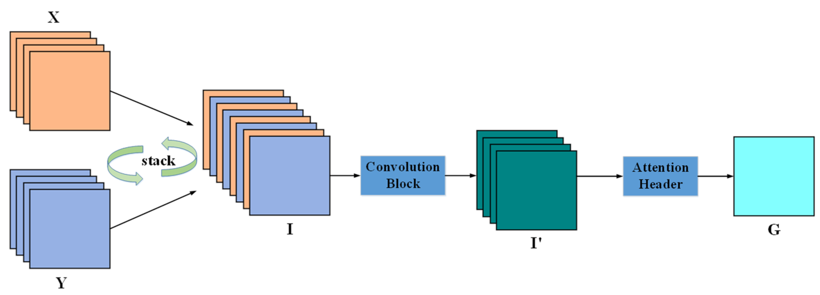
As shown in Figure 4, and represent the output features from the feature alignment module. The features X and Y have the same C, H, and W and the same feature order, which indicates that the channel information of X and the corresponding channel information of Y have the same semantic relationship. Therefore, channel stacking is performed on features X and Y to obtain the feature map as shown in Expression (3):
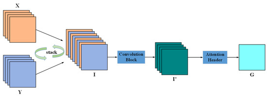
Figure 4.
Structure of cross-mixing attention module.
Passing through a convolution block, the feature map I fuses the spatial and channel features of X and Y, using their semantic similarity. Firstly, I undergoes a depth-wise separable convolution operation to effectively capture both the channel and spatial feature information of I. Then, PReLU activation and instance normalization operations are performed to obtain new features, as shown in Expression (4):
where and represent the number of input and output channels, respectively.
contains the spatiotemporal information of the feature map and is processed using a per-pixel attention header to generate the attention weight map. The attention header consists of a 6-layer 1 × 1 convolutional kernel and a PReLU activation function. By passing through the attention head, channel compression and activation operations are performed to obtain the attention weight map .
2.4. Cross-Mixing Module and Guiding Up-Sampling
Convolutional neural networks commonly employ skip connections for channel splicing, leading to the fusion of considerable redundant information. During decoding, interpolation serves as the typical method for direct feature map up-sampling. However, this parameterless, unlearnable approach often results in blurred target edges. To address this issue, cross-mixing attention weight maps guide the up-sampling process. Initially, up-sampling fused feature maps from stage 4 aligns their size with those of stage 3. Subsequently, these up-sampled maps undergo per-pixel multiplication with the attention maps from stage 3, resulting in new feature maps. This process captures Stage 3’s feature information, balancing global feature relationships and compensating for the non-learnable disadvantage of up-sampling. This process is executed layer by layer to restore the feature map to its initial size.
2.5. Loss Function
As the change detection problem is essentially a binary classification task, we employed the Binary Cross Entropy loss function as follows:
Here, N represents the number of samples; denotes the true label; and represents the predicted probability value for the change region.
3. Datasets and Model Evaluation Indicators
3.1. Remote Image Datasets
The LEVIR-CD dataset comprises 637 pairs of high-resolution satellite remote sensing images, each with a spatial resolution of 0.5 m and an image size of 1024 pixels by 1024 pixels. A source of high-resolution remote sensing images is Google Earth (GE), and the image patch pairs are obtained through the Google Earth API. The dataset images contain three types of spectral information, namely red, green, and blue. These images were primarily collected from Texas, USA, focusing on building structures. Each image pair represents a time span ranging from 5 to 14 years, including four seasons. The analysis area of each image is 32,768 square meters. During dataset preparation, the images were cropped to 256 pixels × 256 pixels, and then partitioned into subsets. Specifically, the training set comprised 7120 pairs of images, the validation set contained 1024 pairs, and 2048 pairs were allocated to the test set. LEVIR-CD: LEVIR Building Change Detection dataset. This dataset was created by a team from Beihang University. Note that LEVIR is the name of the dataset authors’ laboratory: the Learning, Vision, and Remote Sensing Laboratory.
On the other hand, the SYSU-CD dataset includes 20,000 pairs of aerial photographs, each with a resolution of 256 pixels by 256 pixels. The dataset images contain three types of spectral information (i.e., red, green, and blue), with an analysis area of 32,768 square meters and a spatial resolution of 0.5 m for each image. Captured from Hong Kong, China, these images exhibit diverse features, including buildings, vegetation, roads, and marine structures. The data collection period spans from 2007 to 2014, including four seasons. This dataset is split into subsets using a ratio of 6:2:2, with 12,000 pairs in the training set, 4000 pairs in the validation set, and another 4000 pairs assigned to the test set. SYSU-CD: Sun Yat-Sen University Change Detection dataset. SYUS refers to the work unit name of the dataset author, Sun Yat-Sen University.
Compared with multispectral data, the LEVIR-CD dataset has relatively poor spectral information (i.e., red, green, and blue). But the high-resolution image of the LEVIR-CD dataset provides fine texture and geometry information, which, to some extent, compensates for the limitation of poor spectral characteristics. The SYSU-CD dataset also has relatively poor spectral information (i.e., red, green, and blue), but it greatly supplements the existing CD dataset in terms of change types and data volume.
This article focuses on detecting changes in artificial objects in the network, so we selected the LEVIR-CD dataset and the SYSU-CD dataset to validate our network. Among them, the LEVIR-CD dataset only includes changes in artificial buildings and does not consider other types of changes. To verify the robustness of the model proposed in this article, a more complex SYSU-CD dataset was used, which includes features such as buildings, vegetation, roads, and offshore construction.
3.2. Model Evaluation Indicators
In the experiment, five metrics [44] such as precision (Pr), recall (Rc), the F1 score (F1s), Intersection over Union (IoU), and Overall Accuracy (OA) were used to evaluate the performance of the network. In change detection tasks, the higher the accuracy value, the fewer false positives there are in the predicted results. The larger the recall value, the fewer times the predicted result is missed. The F1 score and IoU are comprehensive evaluation indicators for prediction results, and the higher their values, the better the network performance. The higher the accuracy value, the greater the proportion of correct prediction results to the total amount. This is shown in Expressions (6)–(10):
Here, TP represents the count of pixels predicted to be changed that is indeed changed, TN denotes the count of pixels predicted to be unchanged that is indeed unchanged, FP signifies the count of pixels predicted to be changed but is actually unchanged, and FN indicates the count of pixels predicted to be unchanged but is actually changed.
4. Experimental Design and Results Discussion
The network proposed in this paper was implemented using the PyTorch deep learning framework (version: 1.7.1). The experiments were conducted on a 64-bit Windows 10 server system equipped with an Intel Xeon R processor E5-2650 v4 (2.20 GHz) CPU and 80 GB of RAM. An Nvidia GeForce GTX 1080 Ti graphics card with 11 GB of video memory was utilized.
For the training process, the AdamW optimization algorithm was employed with an initial learning rate set to 0.0032, a weight decay coefficient of 0.0095, a network batch size of eight, and trained over 300 epochs. A CosineAnnealingLR strategy dynamically adjusted the learning rate, as illustrated in Expression (11):
where is the current learning rate, is the minimum value of the learning rate, is the maximum value of the learning rate, is the current number of iterations, and is the maximum number of iterations.
The experimental procedure encompasses ablation and comparison experiments, highlighting the optimal index value, as indicated in bold. Table 1 showcases the four abbreviations denoting the proposed experimental strategies. Specifically, the BL (baseline) signifies the Siamese inputs where the backbone network constitutes a deep convolutional encoding–decoding network of EfficientNetB4. This backbone network receives dual temporal images as input, with an image size of 256 pixels × 256 pixels.

Table 1.
Abbreviation for model type.
4.1. Ablation Experiments on the LEVIR-CD Dataset
The network’s module validity is systematically confirmed through step-by-step experiments conducted on the LEVIR-CD dataset. Table 2 exhibits the quantitative metrics derived from the ablation experiments performed on the LEVIR-CD dataset, while Figure 5 showcases a selection of predicted results.
Table 2.
Results of ablation experiments on LEVIR-CD dataset. Bold font represents the optimal value for each column.
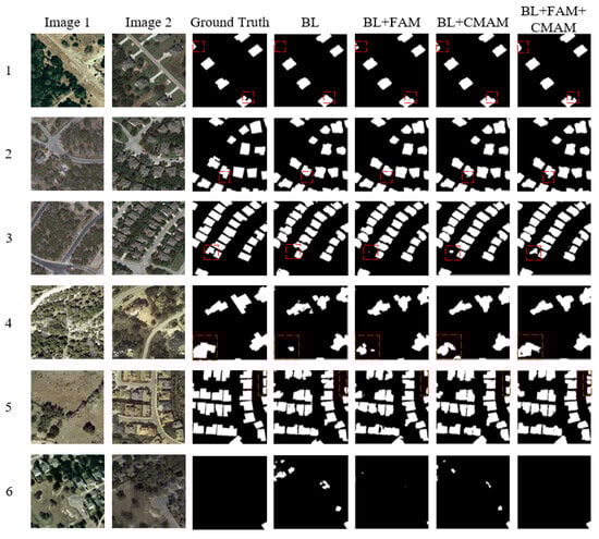
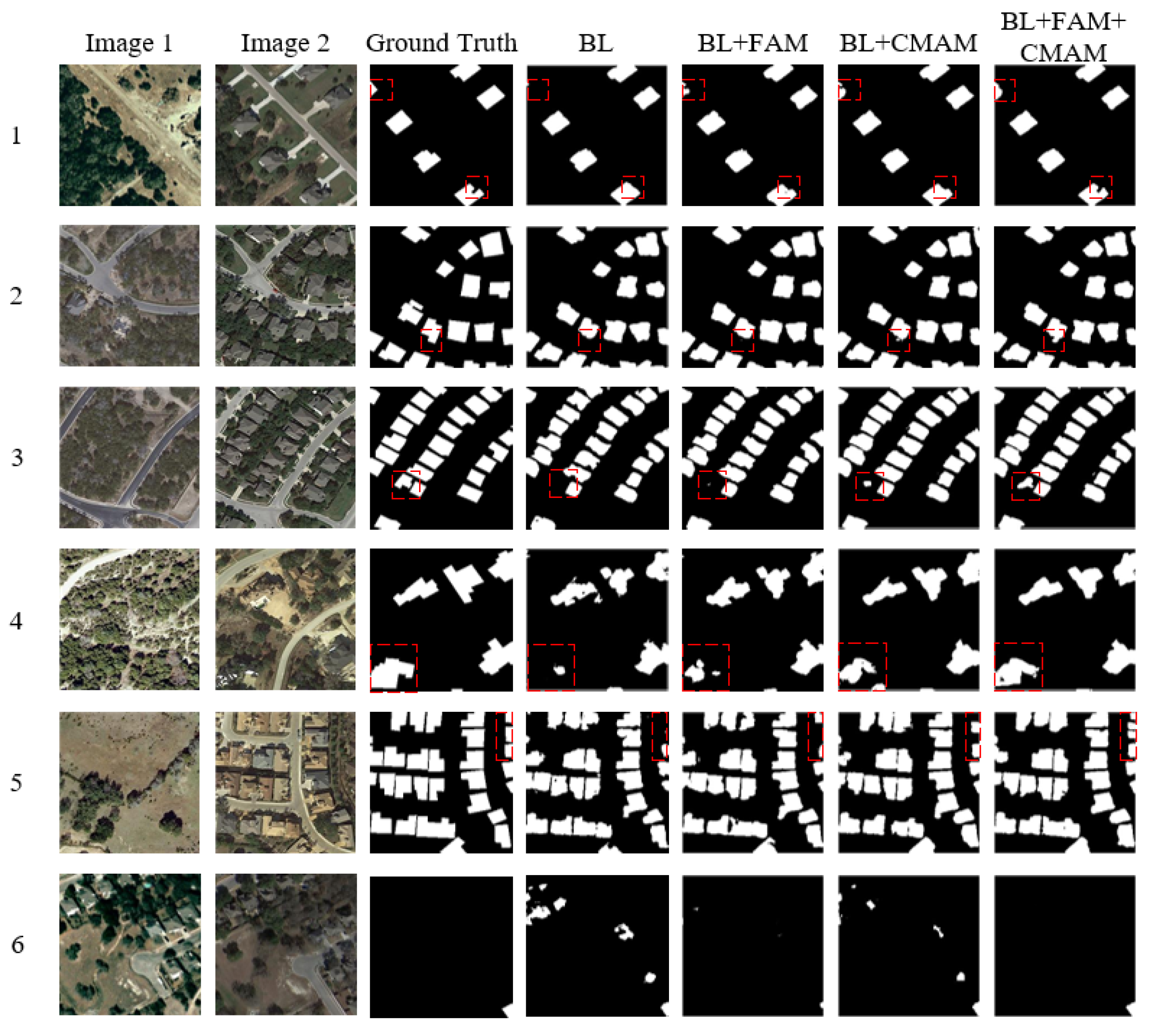
Figure 5.
Partial predictions of ablation experiments on LEVIR-CD dataset. The red boxes are drawn to highlight the advantages of our modules. The numbers 1–6 represent 6 sets of experimental results.
4.1.1. Results of Ablation Experiments with Increased FAM
Table 2 illustrates how integrating the FAM module into BL results in improvements of 0.31% in Pr, 1.19% in Rc, 0.78% in F1s, 1.28% in IoU, and 0.03% in OA compared to BL. Observing the prediction plot in column 5 of Figure 5 reveals that BL + FAM effectively minimizes false detections along the spatial edges of buildings. Thus, via the feature alignment mechanism, it adeptly mitigates feature map misalignment or parallax induced by alignment errors in the dual-temporal image, consequently enhancing change detection accuracy.
4.1.2. Results of Ablation Experiments with Increased CMAM
Table 2 illustrates how integrating the CMAM module into BL results in improvements of 0.33% in Pr, 3.16% in Rc, 1.79% in F1s, 2.94% in IoU, and 0.06% in OA compared to BL. Conversely, the comparison of BL + FAM indicates increases of 0.02% in Pr, 1.97% in Rc, 1.01% in F1s, 1.66% in IoU, and 0.03% in OA. This implies that the overall performance of BL + CMAM surpasses that of BL + FAM. Observing the prediction graph in column 6 of Figure 5 reveals that BL + CMAM adeptly integrates information from the dual-temporal phase images, enhancing the identification of global information. Nonetheless, local spatial information misidentification occurs due to alignment errors, causing the identification of some shadows as changing regions.
4.1.3. Results of Ablation Experiments with Increased FAM and CMAM
Table 2 indicates how incorporating FAM and CMAM into BL results in BL + FAM increasing by 0.92% in Pr, 2.18% in Rc, 1.56% in F1s, 2.59% in IoU, and 0.10% in OA. On the other hand, BL + CMAM exhibited increases of 0.90% in Pr, 0.21% in Rc, 0.55% in F1s, 0.93% in IoU, and 0.07% in OA. The observation from Figure 5 highlights how BL + FAM + CMAM amalgamates the strengths of both FAM and CMAM, resulting in predicted outcomes closer to the ground truth. Consequently, this minimizes the false detections and missed detections induced by building shadows and misaligned edges while enhancing global information through dual-temporal feature fusion, thereby elevating the detection accuracy across the overall target area. BL + FAM + CMAM demonstrates enhanced capability in addressing remote sensing image change detection tasks.
4.2. Ablation Experiments on the SYSU-CD Dataset
The functionality of every module in the network undergoes systematic verification via experiments conducted on the LEVIR-CD dataset. Table 3 displays the quantitative metrics derived from the ablation experiments conducted on the LEVIR-CD dataset, while Figure 6 depicts a subset of the predicted outcomes.
Table 3.
Results of ablation experiments on SYSU-CD dataset. Bold font represents the optimal value for each column.
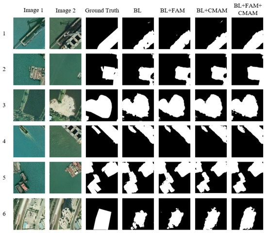
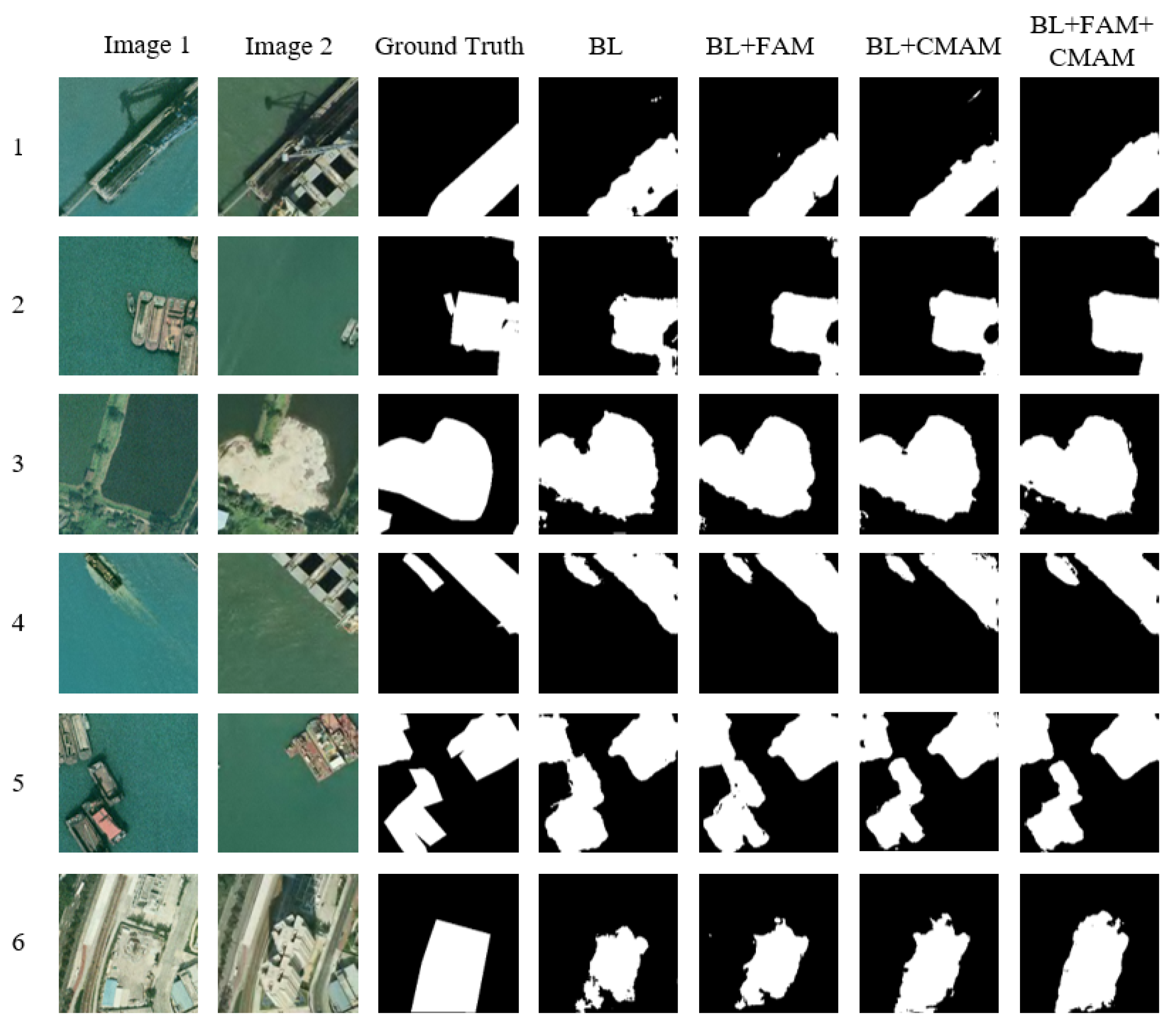
Figure 6.
Partial predictions of ablation experiments on SYSU-CD dataset. The numbers 1–6 represent 6 sets of experimental results.
4.2.1. Results of Ablation Experiments with Increased FAM
Table 3 illustrates how integrating the FAM module into BL results in an increase of 3.18% in Pr, 3.69% in Rc, 1.66% in F1s, 2.26% in IoU, and 0.49% in OA, compared to BL. Observing the prediction graph in column 5 of Figure 6 reveals that the feature alignment mechanism enhances the ability for local edge feature integration, effectively mitigating the feature map misalignment or parallax issues resulting from alignment errors in the dual-temporal phase image and consequently enhancing change detection accuracy.
4.2.2. Results of Ablation Experiments with Increased CMAM
Table 3 demonstrates how incorporating the CMAM module into BL results in increases of 1.14% in Pr, 5.35% in Rc, 2.16% in F1, 2.95% in IoU, and 0.64% in OA compared to BL. In comparison with BL + FAM, it registers increases of 1.66% in Rc, 0.50% in F1, 0.69% in IoU, and 0.15% in OA, with a decrease of 2.04% in Pr. Consequently, although BL + CMAM outperforms BL + FAM overall, there is an increase in false positives. The predicted outcomes in columns 5 and 6 of Figure 6 highlight BL + CMAM’s strengths in global target area recognition. However, registration errors result in the incorrect identification of boundary position information within the target area.
4.2.3. Results of Ablation Experiments with Increased FAM and CMAM
Table 3 highlights how incorporating both FAM and CMAM into BL results in improvements of 4.31% in Pr, 4.03% in Rc, 2.33% in F1s, 3.27% in IoU, and 2.63% in OA. Comparatively, against BL + FAM, it shows increases of 6.35% in Pr, 2.37% in Rc, and 2.37% in F1s, IoU, and OA, and 1.83%, 2.58%, and 2.48%. Figure 6 demonstrates how BL + FAM + CMAM outperforms BL + FAM and BL + CMAM in change detection performance. Feature alignment mitigates the false detections caused by alignment errors, while dual-temporal phase feature fusion enables the complementation of spatiotemporal information between dual-temporal phase images, enhancing change discrimination and reducing detection omissions.
4.3. Comparison Experiments on the LEVIR-CD Dataset
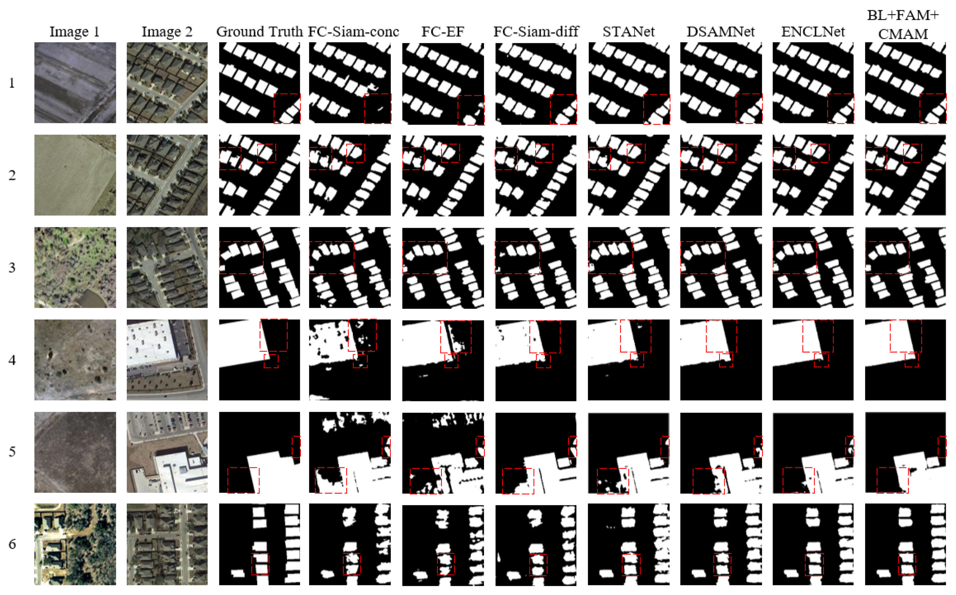
To validate the model’s efficacy, BL + FAM + CMAM is compared against six networks using the LEVIR-CD dataset. Table 4 and Figure 7 display the selected prediction results and quantitative metrics derived from the LEVIR-CD dataset. Observing Figure 7 reveals how the FC-EF, FC-Siam-diff, and FC-Siam-conc display have more missed and mis-detected segments attributed to inadequate feature extraction in the codec stage and suboptimal feature integration. Conversely, the remaining four methods successfully detect the primary building change contours, demonstrating their capacity to represent building change features. ENCLNet and BL + FAM + CMAM yield more comprehensive building change boundaries, suggesting superior change detection performance for these models.
Table 4.
Quantitative comparison with 6 methods on LEVIR-CD dataset. Bold font represents the optimal value for each column.
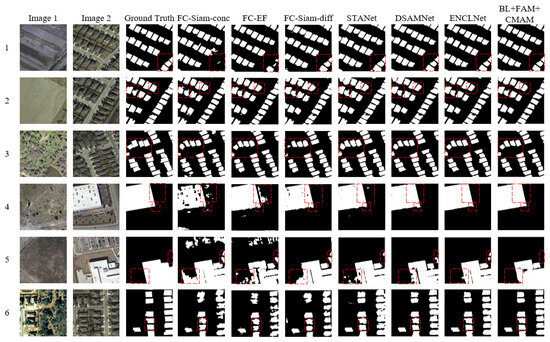
Figure 7.
Partial prediction results of comparative experiments on the LEVIR-CD dataset. The red boxes are drawn to highlight the advantages of our modules. The numbers 1–6 represent 6 sets of experimental results.
Table 4 quantitatively demonstrates the change detection performance metrics of the seven models. FC-Siam-conc achieves an F1 score of 78.36%, while FC-EF and FC-Siam-diff attain 79.34% and 82.03%, respectively. FC-EF’s precision stands at 79.49% due to elevated false positives, while FC-Siam-conc records a recall of 76.76% due to higher misses. FC-Siam-diff exhibits a 3.64% increase in precision over FC-EF and a 4.21% rise in recall over FC-Siam-conc. The FC-Siam-diff architecture proves more adept at change detection, showcasing the twin network’s improved ability to extract features from both images. ENCLNet demonstrates remarkable change detection capabilities by adaptively identifying differences and consistencies in bi-chronological features, achieving a noteworthy F1 score of 90.06% via the building edge neighborhood comparison learning method. Compared with the F1 scores obtained using FC-Siam-conc, FC-EF, FC-Siam-diff, STANet, DSAMNet, and ENCLNet, the F1 scores of BL + FAM + CMAM increased by 12.70%, 11.72%, 9.03%, 4.29%, 3.55%, and 1.00%, respectively, yielding the highest detection results. As shown in Figure 7, BL + FAM + CMAM yielded the clearest building change boundaries and the most complete overall building change. This verifies the effectiveness of the proposed method in eliminating alignment errors, the feature fusion interaction of dual-temporal images, and improving the overall performance of change detection.
4.4. Comparison Experiments on the SYSU-CD Dataset
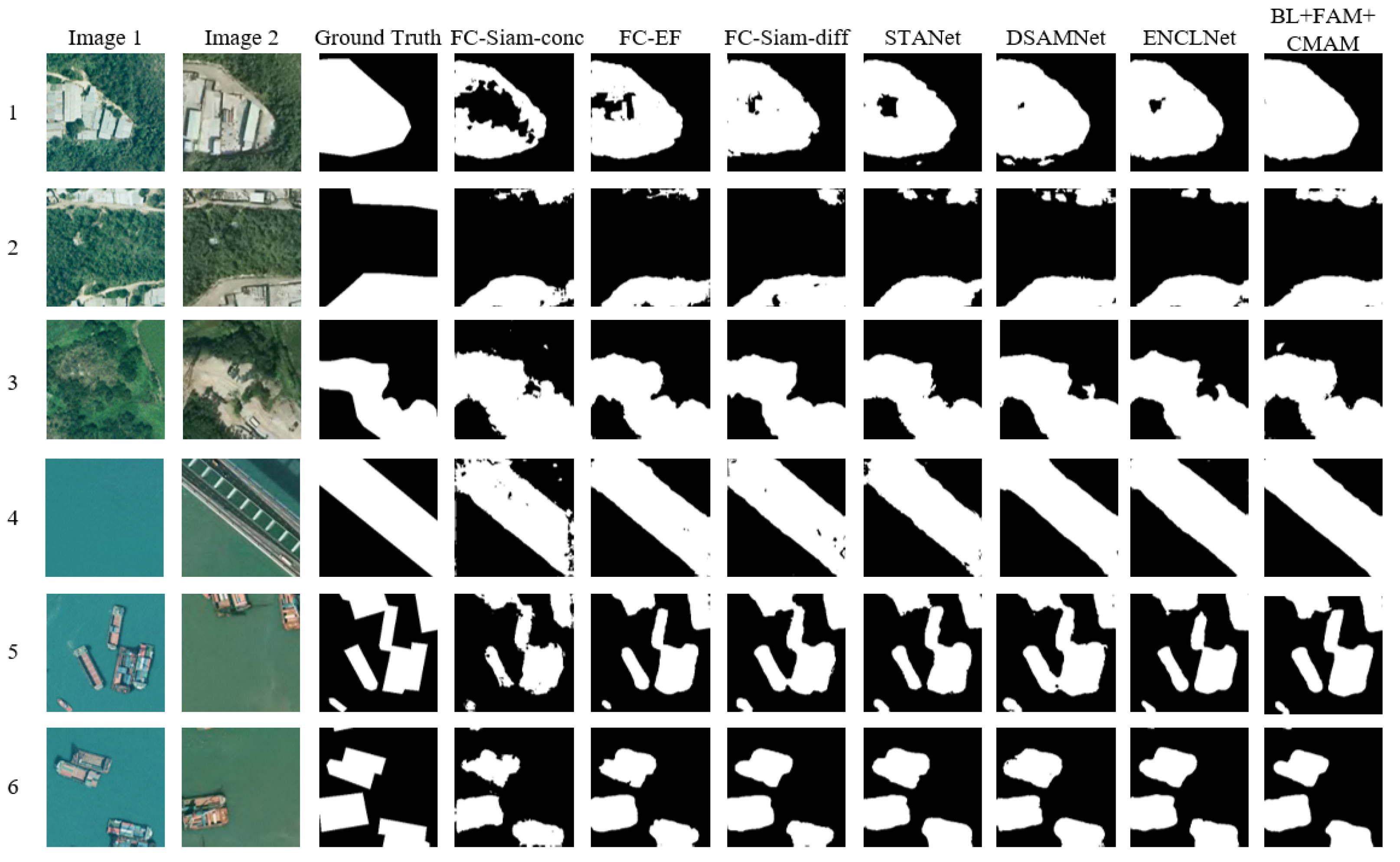
To assess the model’s validity, BL + FAM + CMAM was compared with six networks using the SYSU-CD dataset. A subset of prediction results and quantitative metrics from the SYSU-CD dataset is depicted in Figure 8 and Table 5.
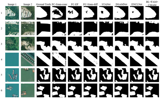
Figure 8.
Partial prediction results of comparative experiments on SYSU-CD dataset. The numbers 1–6 represent 6 sets of experimental results.
Table 5.
Quantitative comparison with 6 methods on SYSU-CD dataset. Bold font represents the optimal value for each column.
Observations akin to those in the LEVIR-CD dataset are evident in Figure 8. The main changes can be detected using FC-Siam-conc, FC-EF, and FC-Siam-diff, but they exhibit numerous false positives and missed detections. STANet and DSAMNet demonstrate improved detection performance through adaptive multi-scale feature fusion, spatiotemporal attention mechanisms, deep supervision, and CBAM integration. ENCLNet obtains suboptimal detection results using adaptive selective attention and edge neighborhood comparison learning methods. BL + FAM + CMAM yielded the best detection results, showcasing relatively comprehensive changes in the regions.
Table 4 and Table 5 illustrate that the accuracy of the seven models on the SYSU-CD dataset is generally lower compared to the LEVIR-CD dataset. The LEVIR-CD dataset primarily identifies changes in buildings, presenting fewer change types and a simpler background. Conversely, the SYSU-CD dataset includes changes in roads, vegetation, buildings, ships, etc., featuring diverse change types and complex backgrounds. Among the models, BL + FAM + CMAM achieved optimal performance, demonstrating its effectiveness in feature extraction, fusion, weight allocation, and acquiring semantic information from dual temporal features, with precision (Pr), recall (Rc), F1 score (F1), Intersection over Union (IoU), and Overall Accuracy (OA) indicators at 84.15%, 79.73%, 81.88%, 69.32%, and 88.32%, respectively. This underscores BL + FAM + CMAM’s robustness in handling datasets with complex backgrounds and various types of changes.
5. Conclusions and Future Works
This paper introduces a novel network model employing cross-mixed attention for the detection of changes in remote sensing images. This network comprises a feature alignment module (FAM) and a cross-mixing attention module (CMAM) as its primary components. The FAM rectifies alignment errors by repositioning pixel coordinates in dual-temporal phase feature maps, reducing false detections attributed to alignment errors. Meanwhile, the CMAM produces multi-scale weight maps for guiding the up-sampling process, facilitating the introduction of detailed information and enabling learnability in the up-sampling. Ablation and comparative experiments are conducted on two datasets (LEVIR-CD and SYSU-CD). The image source of the LEVIR-CD dataset is Google Earth, which is a high-resolution satellite remote sensing image containing three types of spectral information (i.e., red, green, and blue). The image source of the SYSU-CD dataset is drone aerial photography, which contains three types of spectral information (i.e., red, green, and blue). The experimental results show that, under the same experimental conditions compared with six change detection methods, the proposed network performs well on the LEVIR-CD and SYSU-CD datasets, with F1 scores of 91.06% and 81.88%, respectively. The proposed network not only reduces the false detection of changing target contours but also improves the detection accuracy of target objects at different scales, and the overall effect is better than the compared network. Given the challenge in labeling remote sensing image change detection datasets, future research should explore training the network with weakly supervised learning methods to enhance dataset detection accuracy and network robustness.
Author Contributions
Conceptualization, C.W. and L.Y.; methodology, C.G.; software, X.W.; writing—original draft preparation, L.Y.; writing—review and editing, X.W. All authors have read and agreed to the published version of the manuscript.
Funding
This research was funded by the Planned project of Gansu science and Technology Department under Contract 21JR7RA310, the Science and Technology Planning Project of Chengguan District of Lanzhou City under Contract 2019-5-1, and the Youth Science Fund Project of Lanzhou Jiaotong University under Contract 2021029, Gansu Science and Technology Program (Key Research and Development Program) under Contract 20YF8GA035.
Data Availability Statement
The data that support the findings of this study are available on request from the corresponding author.
Acknowledgments
We thank the associate editor and the reviewers for their useful feedback that improved this paper.
Conflicts of Interest
The authors declare no conflicts of interest.
References
- Zhang, Z.X.; Jiang, H.W.; Pang, S.Y.; Hu, X. Review and prospect in change detection of mult-temporal remotesensing images. Acta Geod. Cartogr. Sin. 2022, 51, 1091–1107. [Google Scholar]
- Schaum, A. Local covariance equalization of hyperspectral imagery: Advantages and limitations for target detection. In Proceedings of the 2005 IEEE Aerospace Conference, Big Sky, MT, USA, 5–12 March 2005; pp. 2001–2011. [Google Scholar]
- Pourreza, M.; Moradi, F.; Khosravi, M.; Deljouei, A.; Vanderhoof, M.K. GCPs-free photogrammetry for estimating tree height and crown diameter in Arizona Cypress plantation using UAV-mounted GNSS RTK. Forests 2022, 13, 1905. [Google Scholar] [CrossRef]
- Moradi, F.; Darvishsefat, A.A.; Pourrahmati, M.R.; Deljouei, A.; Borz, S.A. Estimating aboveground biomass in dense Hyrcanian forests by the use of Sentinel-2 data. Forests 2022, 13, 104. [Google Scholar]
- Eismann, M.T.; Meola, J.; Hardie, R.C. Hyperspectral change detection in the presenceof diurnal and seasonal variations. IEEE Trans. Geosci. Remote Sens. 2007, 46, 237–249. [Google Scholar] [CrossRef]
- Zhou, J.; Kwan, C.; Ayhan, B.; Eismann, M.T. A novel cluster kernel RX algorithm for anomaly and change detection using hyperspectral images. IEEE Trans. Geosci. Remote Sens. 2016, 54, 6497–6504. [Google Scholar] [CrossRef]
- Radke, R.J.; Andra, S.; Al-Kofahi, O.; Roysam, B. Image change detection algorithms: A systematic survey. IEEE Trans. Image Process. 2005, 14, 294–307. [Google Scholar] [CrossRef] [PubMed]
- İlsever, M.; Ünsalan, C. Two-Dimensional Change Detection Methods: Remote Sensing Applications; Springer Science & Business Media: Berlin, Germany, 2012. [Google Scholar]
- Kwan, C. Methods and challenges using multispectral and hyperspectral images for practical change detection applications. Information 2019, 10, 353. [Google Scholar] [CrossRef]
- Amare, M.T.; Demissie, S.T.; Beza, S.A.; Erena, S.H. Land Cover Change Detection and Prediction in the Fafan Catchment of Ethiopia. J. Geovisualization Spat. Anal. 2023, 7, 19. [Google Scholar] [CrossRef]
- Daudt, R.C.; Le Saux, B.; Boulch, A.; Gousseau, Y. Urban change detection for multispectral earth observation using convolutional neural networks. In Proceedings of the IGARSS 2018 IEEE International Geoscience and Remote Sensing Symposium, Valencia, Spain, 22–27 July 2018; pp. 2115–2118. [Google Scholar]
- Gupta, R.; Hosfelt, R.; Sajeev, S.; Patel, N.; Goodman, B.; Doshi, J.; Heim, E.; Choset, H.; Gaston, M. xbd: A dataset for assessing building damage from satellite imagery. arXiv 2019, arXiv:1911.09296. [Google Scholar]
- Jiang, J.; Xiang, J.; Yan, E.; Song, Y.; Mo, D. Forest-CD: Forest Change Detection Network Based on VHR Images. IEEE Geosci. Remote Sens. Lett. 2022, 19, 2506005. [Google Scholar] [CrossRef]
- Celik, T. Unsupervised change detection in satellite images using principal component analysis and k-means clustering. IEEE Geosci. Remote Sens. Lett. 2009, 6, 772–776. [Google Scholar] [CrossRef]
- Jia, L.; Li, M.; Zhang, P.; Wu, Y.; An, L.; Song, W. Remote-sensing image change detection with fusion of multiple wavelet kernels. IEEE J. Sel. Top. Appl. Earth Obs. Remote Sens. 2016, 9, 3405–3418. [Google Scholar] [CrossRef]
- Wang, M.J.; Huang, L. Change detection method of multi-temp-oral remote sensing images based on dual-threshold exponent information entropy. Remote Sens. Inf. 2017, 32, 81–85. [Google Scholar]
- EI Amin, A.M.; Liu, Q.; Wang, Y. Convolutional neural network features based change detection in satellite images. In Proceedings of the First International Workshop on Pattern Recognition, Tokyo, Japan, 11–13 May 2016; Volume 10011, pp. 181–186. [Google Scholar]
- Krizhevsky, A.; Sutskever, I.; Hinton, G.E. Imagenet classification with deep convolutional neural networks. Commun. ACM 2017, 60, 84–90. [Google Scholar] [CrossRef]
- Li, S.; Song, W.; Fang, L.; Chen, Y.; Ghamisi, P.; Benediktsson, J.A. Deep learning for hyperspectral image classification: An overview. IEEE Trans. Geosci. Remote Sens. 2019, 57, 6690–6709. [Google Scholar] [CrossRef]
- Khelifi, L.; Mignotte, M. Deep learning for change detection in remote sensing images: Comprehensive review and meta-analysis. IEEE Access 2020, 8, 126385–126400. [Google Scholar] [CrossRef]
- LeCun, Y.; Bengio, Y.; Hinton, G. Deep learning. Nature 2015, 521, 436–444. [Google Scholar] [CrossRef]
- Zhu, X.X.; Tuia, D.; Mou, L.; Xia, G.-S.; Zhang, L.; Xu, F.; Fraundorfer, F. Deep learning in remote sensing: A comprehensive review and list of resources. IEEE Geosci. Remote Sens. Mag. 2017, 5, 8–36. [Google Scholar] [CrossRef]
- Shi, W.; Zhang, M.; Zhang, R.; Chen, S.; Zhan, Z. Change detection based on artificial intelligence: State-of-the-art and challenges. Remote Sens. 2020, 12, 1688. [Google Scholar] [CrossRef]
- Daudt, R.C.; Le Saux, B.; Boulch, A. Fully convolutional siamese networks for change detection. In Proceedings of the 2018 25th IEEE International Conference on Image Processing (ICIP), Athens, Greece, 7–10 October 2018; pp. 4063–4067. [Google Scholar]
- Long, J.; Shelhamer, E.; Darrell, T. Fully convolutional networks for semantic segmentation. In Proceedings of the IEEE Conference on Computer Vision and Pattern Recognition, Boston, MA, USA, 7–12 June 2015; pp. 3431–3440. [Google Scholar]
- Bromley, J.; Guyon, I.; Lecun, Y.; Säckinger, E.; Shah, R. Signature verification using a “siamese” time delay neural network. Adv. Neural Inf. Process. Syst. 1993, 7, 669–688. [Google Scholar] [CrossRef]
- Zhou, Z.; Rahman Siddiquee, M.M.; Tajbakhsh, N.; Liang, J. Unet++: A nested u-net architecture for medical image segmentation. Deep Learning in Medical Image Analysis and Multimodal Learning for Clinical Decision Support: 4th International Workshop. In Proceedings of the DLMIA 2018, and 8th International Workshop, ML-CDS 2018, Held in Conjunction with MICCAI 2018, Granada, Spain, 20 September 2018; Springer International Publishing: Cham, Switzerland, 2018; pp. 3–11. [Google Scholar]
- Peng, D.; Zhang, Y.; Guan, H. End-to-end change detection for high resolution satellite images using improved UNet++. Remote Sens. 2019, 11, 1382. [Google Scholar] [CrossRef]
- Han, P.; Ma, C.; Bu, S.; Chen, L.; Xia, Z.; Hu, J. Correlation and Attention Mechanism based Network for Change Detection. In Proceedings of the 2022 China Automation Congress (CAC), Xiamen, China, 25–27 June 2022; pp. 3268–3273. [Google Scholar]
- Ma, L.; Wang, L.; Zhao, C.; Ohtsuki, T. Multilayer Attention Mechanism for Change Detection in SAR Image Spatial-Frequency Domain. In Proceedings of the 2023 IEEE International Conference on Image Processing (ICIP), Kuala Lumpur, Malaysia, 8–11 October 2023; pp. 2110–2114. [Google Scholar]
- Chen, J.; Yuan, Z.; Peng, J.; Chen, L.; Huang, H.; Zhu, J.; Liu, Y.; Li, H. DASNet: Dual attentive fully convolutional siamese networks for change detection of high resolution satellite images. IEEE J. Sel. Top. Appl. Earth Obs. Remote Sens. 2020, 14, 1194–1206. [Google Scholar] [CrossRef]
- Shi, Q.; Liu, M.; Li, S.; Liu, X.; Wang, F.; Zhang, L. A deeply supervised attention metric-based network and an open aerial image dataset for remote sensing change detection. IEEE Trans. Geosci. Remote Sens. 2021, 60, 5604816. [Google Scholar] [CrossRef]
- Woo, S.; Park, J.; Lee, J.Y.; Kweon, I.S. Cbam: Convolutional block attention module. In Proceedings of the European Conference on Computer Vision (ECCV), Munich, Germany, 8–14 September 2018; pp. 3–19. [Google Scholar]
- Chen, H.; Shi, Z. A spatial-temporal attention-based method and a new dataset for remote sensing image change detection. Remote Sens. 2020, 12, 1662. [Google Scholar] [CrossRef]
- Zhang, M.; Li, Q.; Yuan, Y.; Wang, Q. Edge Neighborhood Contrastive Learning for Building Change Detection. IEEE Geosci. Remote Sens. Lett. 2022, 20, 6001305. [Google Scholar] [CrossRef]
- Chen, L.C.; Papandreou, G.; Kokkinos, I.; Murphy, K.; Yuille, A.L. Deeplab: Semantic image segmentation with deep convolutional nets, atrous convolution, and fully connected crfs. IEEE Trans. Pattern Anal. Mach. Intell. 2017, 40, 834–848. [Google Scholar] [CrossRef] [PubMed]
- Sun, K.; Xiao, B.; Liu, D.; Wang, J. Deep high-resolution representation learning for human pose estimation. In Proceedings of the IEEE/CVF Conference on Computer Vision and Pattern Recognition, Long Beach, CA, USA, 15–20 June 2019; pp. 5693–5703. [Google Scholar]
- Zhao, H.; Shi, J.; Qi, X.; Wang, X.; Jia, J. Pyramid scene parsing network. In Proceedings of the IEEE Conference on Computer Vision and Pattern Recognition, Honolulu, HI, USA, 21–26 July 2017; pp. 2881–2890. [Google Scholar]
- Ou, X.; Liu, L.; Tu, B.; Zhang, G.; Xu, Z. A CNN framework with slow-fast band selection and feature fusion grouping for hyperspectral image change detection. IEEE Trans. Geosci. Remote Sens. 2022, 60, 5524716. [Google Scholar] [CrossRef]
- Shen, Q.; Huang, J.; Wang, M.; Zhang, G.; Xu, Z. Semantic feature-constrained multitask siamese network for building change detection in high-spatial-resolution remote sensing imagery. ISPRS J. Photogramm. Remote Sens. 2022, 189, 78–94. [Google Scholar] [CrossRef]
- Tan, M.; Le, Q. Efficientnet: Rethinking model scaling for convolutional neural networks. In Proceedings of the International Conference on Machine Learning, Long Beach, CA, USA, 9–15 June 2019; pp. 6105–6114. [Google Scholar]
- Jaderberg, M.; Simonyan, K.; Zisserman, A. Spatial transformer networks. Adv. Neural Inf. Process. Syst. 2015, 28, 2017–2025. [Google Scholar]
- Chollet, F. Xception: Deep learning with depthwise separable convolutions. In Proceedings of the IEEE Conference on Computer Vision and Pattern Recognition, Honolulu, HI, USA, 21–26 July 2017; pp. 1251–1258. [Google Scholar]
- El Naqa, I.; Murphy, M.J. What is Machine Learning? In Machine Learning in Radiation Oncology; Springer International Publishing: Cham, Switzerland, 2015. [Google Scholar]


Disclaimer/Publisher’s Note: The statements, opinions and data contained in all publications are solely those of the individual author(s) and contributor(s) and not of MDPI and/or the editor(s). MDPI and/or the editor(s) disclaim responsibility for any injury to people or property resulting from any ideas, methods, instructions or products referred to in the content. |
© 2024 by the authors. Licensee MDPI, Basel, Switzerland. This article is an open access article distributed under the terms and conditions of the Creative Commons Attribution (CC BY) license (https://creativecommons.org/licenses/by/4.0/).