Popularity-Debiased Graph Self-Supervised for Recommendation

Abstract

The rise of graph neural networks has greatly contributed to the development of recommendation systems, and self-supervised learning has emerged as one of the most important approaches to address sparse interaction data. However, existing methods mostly focus on the recommendation’s accuracy while neglecting the role of recommended item diversity in enhancing user interest and merchant benefits. The reason for this phenomenon is mainly due to the bias of popular items, which makes the long-tail items (account for a large proportion) be neglected. How to mitigate the bias caused by item popularity has become one of the hot topics in current research. To address the above problems, we propose a Popularity-Debiased Graph Self-Supervised for Recommendation (PDGS). Specifically, we apply a penalty constraint on item popularity during the data enhancement process on the user–item interaction graph to eliminate the inherent popularity bias. We generate item similarity graphs with the popularity bias removed to construct a self-supervised learning task under multiple views, and we design model optimization strategies from the perspectives of popular items and long-tail items to generate recommendation lists. We conduct a large number of comparison experiments, as well as ablation experiments, on three public datasets to verify the effectiveness and the superiority of the model in balancing recommendation accuracy and diversity.

1. Introduction

In recent years, recommendation systems (RS) have emerged in order to mitigate the effect of information overload. Due to the advantages in improving platform effectiveness and user satisfaction, recommendation systems are widely applied in various industries. Recommendation systems aim to mine user preferences based on the observed interaction data and provide personalized services/items to users.

With the rise of deep learning, researchers have attempted to model users’ and items’ representations in recommendation data with graph neural networks. However, these approaches heavily rely on sufficient interaction data [1,2], making them insufficient for addressing data sparsity, noise, etc., in recommendations. Self-supervised learning techniques have been successfully applied in the field of recommendation systems and proved to be effective in alleviating data sparsity issues. Although these methods have shown significant improvements in recommendation accuracy, they have not fully addressed the inherent popularity bias in data augmentation.

In addition, most models focus on recommendation accuracy while neglecting the novelty and diversity of recommended items. At the same time, the unbalanced nature of the observed data makes recommendation systems vulnerable to popularity bias [3]. Specifically, in the observed user–item interactions, users tend to choose the items with high popularity, so the absence of click data does not necessarily imply negative feedback from users [4]. As a result, models tend to recommend popular items to achieve higher recommendation accuracy, which results in a loss of recommendation diversity. This not only affects users’ personalized experience but also affects the potential revenue of item providers, which clearly does not fulfill the requirements of personalized recommendations. The above problems motivate us to safeguard the trade-off between overall recommendation accuracy and debiased recommendation while solving the problems caused by data sparsity and interaction imbalance.

There is significant literature on popularity bias research, which can be mainly categorized into three main types [5]: (1) Data-level, where the reverse propensity score methods adjust the data distribution by reducing the weights of popular items during training [6]. (2) Loss-function-level, where objective approaches balance the popular and long-tail items in recommendation results by increasing the loss function [7]. (3) Model-level, where causal inference approaches utilize counterfactual reasoning to predict user interactions [8]. Although effective, we argue that existing popularity-debiasing methods mostly ignore highly sparse user behavioral data, hindering encoding representation capability.

To address these challenges, we propose PDGS, a popularity-debiased graph self-supervised recommendation algorithm. Specifically, we first define penalty weights for popular and long-tail items based on their popularity, calculate the similarity between items after removing popularity bias, and then construct a popularity-bias-free item similarity graph. We then utilize this graph as an augmented view of the user–item collaboration graph for contrastive learning, thereby alleviating the scarcity of labeled data. Finally, we construct optimization functions from the perspectives of popular and long-tail items to increase the exposure of long-tail items. In summary, our work makes the following contributions:

(1)

We propose a popularity-debiased graph supervised recommendation model (PDGS). We design penalty constraints for items based on their popularity. This graph serves as an augmented view that participates in contrastive learning with the collaborative graph, which compensates for the defect of long-tail items that are less/unrecommended due to exposure limitations.

(2)

We improve the supervised learning recommendation task by considering both popular items and long-tail items and optimize the self-supervised learning task and recommendation task with multitask joint training to achieve end-to-end training of the model to alleviate data sparsity while reducing the impact of popularity bias on model learning, thereby improving recommendation diversity and enhancing user experience.

(3)

We validate the effectiveness of our model through comparative experiments and ablation experiments on three real-world datasets.

2. Related Work

In this section, we review the work relevant to our paper, focusing on two aspects: popularity bias in recommendation systems and self-supervised learning.

2.1. Popularity Bias for Recommendation

Due to the higher attention given to popular items, recommendation systems tend to assign higher rankings to popular items, leading to the problem of popularity bias. On one hand, recommendation systems that ignore popularity and focus solely on data fitting hinder the accuracy, diversity, and novelty of results. This reduces users’ chances of discovering niche products, diminishes user experience, and can result in decreased benefits for service providers [9]. On the other hand, popularity bias leads to the Matthew effect, which leaves more items with low popularity unattended, and the market is occupied by a few high-popularity items [10,11,12], resulting in the homogenization of different user groups [13]. However, compared with popular items, it is more meaningful to recommend more diverse long-tail items for users. Therefore, research on mitigating popularity bias is necessary. Currently, there are several approaches to alleviate popularity bias in recommendation systems: (1) Ranking adjustment. This approach aims to improve the recommendation scores of unpopular items to achieve more balanced recommendations. For example, the IPL [14] introduced a regularization debiasing model based on the proportional interaction between popular and unpopular items and the number of users who like them to obtain unbiased recommendations. (2) Causal inference. This approach analyzes the variables affected by popularity bias during the recommendation process by means of causal graphs or probabilistic derivation so as to implement bias operations. For instance, the DCCL [15] disentangled the cause of clicks into interest and conformity. It directly learned the causal embedding of decoupled users and items on the historical click data, resulting in final recommendations that simultaneously take into account both user interests and conformity. (3) Popularity penalty. This approach aims to measure the similarity between different items for recommendation. For example, Zhang et al. [16] proposed a debiasing method based on popularity and dynamic interest changes. It defined a popularity penalty function based on the difference in popularity between different items to alleviate the high similarity issue of popular items. Additionally, a time-decay function was defined based on users’ behavior characteristics at different times to eliminate popularity bias in historical data.

2.2. Self-Supervised Learning for Recommendation

Self-supervised learning [17] is an emerging paradigm in machine learning. With self-supervised learning, models make full use of relevant information to assist their main task. One branch of self-supervised learning is maximizing mutual information [18,19,20], which has achieved significant progress in computer vision [21], audio processing [22,23], natural language understanding [24], and so on. There are existing works that integrate self-supervised learning with recommendation systems. For example, Zhou et al. [25] leveraged the relevance of contextual information as self-supervision signals in sequence recommendation to maximize the mutual information between attributes, items, and sequence views. Ma et al. [26] maximized the mutual information among items in different temporal sequences.Zou et al. [27] comprehensively considered the semantic and structural relationships between nodes to generate multiple views and proposed a multilevel cross-view contrastive learning mechanism, which achieved local-level contrastive learning between collaborative views and semantic views, as well as global-level contrastive learning between global views and local views.

3. Preliminaries

We first introduce the concepts used in this paper and provide corresponding explanations.

User-Item Graph: Given the sets of M users and N items defined as $\mathit{U}=\{u_1,u_2,\cdots ,u_M\}$ and $\mathit{I}=\{i_1,i_2,\cdots ,i_N\}$, respectively, the interactions between the users and the items are denoted as $\mathbf{Y}\in {\mathbf{R}}^{M\times N}$. Where $y_{ui}=1$, it indicates that there is interaction (e.g., click, purchase, favorite) between the user u and the item i, and vice versa. Therefore, the user–item interaction graph is defined as ${\mathcal{G}}_r=\left\{(u,y_{ui},i)\right|u\in \mathit{U},i\in \mathit{I},y_{ui}\in \mathbf{Y}\}$.

Popularity-Debiased Item Similarity Graph: It is represented as ${\mathcal{G}}_c=\{i,S(i,j),j|i,j\in \mathit{I}\}$. Where, $i,j$ represent the item nodes belonging to ${\mathcal{G}}_c$, we define the item nodes set as $N_c$. If there is a strong correlation between item i and j, then we set $S(i,j)=1$, indicating that there is an edge between item i and item j in graph ${\mathcal{G}}_c$.

Item Popularity: This reflects the overall popularity of items [28], which is often defined as a specific value in research, such as the number of clicks, comments, or other user-related data regarding items.

4. The Proposed Methodology

In this section, we introduce the detailed technical design of our proposed PDGS in Figure 1. Firstly, we construct the inputs for the model, which are the user–item interaction graph (collaborative graph) ${\mathcal{G}}_r$, built based on user–item interaction data, and the item similarity graph ${\mathcal{G}}_c$, obtained by removing the items’ popularity bias. We employ the classical graph neural network LightGCN [29] to learn the node representations, yielding collaborative embeddings for items ${\mathbf{e}}_i^r$ and popularity-debiased embeddings for items ${\mathbf{e}}_i^c$. Then, we leverage the self-supervision signals provided by the interactions between multiple views to construct contrastive learning tasks between the views. Finally, we jointly optimize the self-supervised learning tasks based on popularity debiasing and the recommendation task, creating an end-to-end optimization strategy.

4.1. Popularity-Debiased Item Similarity Graph

User–item interaction behaviors are often influenced by popularity items. Over time, users lose their freshness for uninteracted items, resulting in user churn and incurring incalculable losses. In order to extract the real user preferences and to mitigate the adverse effects caused by the data imbalance during the modeling process of the user–item interaction graph ${\mathcal{G}}_r$, in this section, the item popularity and the popularity difference between items are used to penalize the popularity of the items that users have interacted with. Additionally, a sampling strategy is designed on the basis of the similarity of the penalized weights to generate the popularity-debiased item similarity graph ${\mathcal{G}}_c$. The following section describes in detail the process of constructing graph ${\mathcal{G}}_c$.

Based on the definition of item popularity, its formal expression is denoted as $Po{p}_i=\left|\mathrm{num}{U}_i\right|$. For computational convenience, the item popularity is normalized $f\left(Po{p}_i\right)\in (0,1)$. The formalization process is calculated as follows:

$$nor\text{\_}Po{p}_i=f\left(Po{p}_i\right)=\frac{Po{p}_i-min\text{\_}Pop}{max\text{\_}Pop-min\text{\_}Pop}$$

(1)

where $nor\text{\_}Po{p}_i$ represents the normalized popularity of item i, and $min\text{\_}Pop$ and $max\text{\_}Pop$ denote the minimum and the maximum value of item popularity, respectively.

Then, the popularity difference $Pop\text{\_}Bia{s}_{i,j}$ between item i and item j is calculated by

$$Pop\text{\_}Bia{s}_{i,j}=\left|\begin{array}{c}nor\text{\_}Po{p}_i-nor\text{\_}Po{p}_j\end{array}\right|$$

(2)

The smaller the popularity difference $Pop\text{\_}Bia{s}_{i,j}$, the more similar the popularity between item i and item j, indicating a higher probability of co-occurrence in the candidate recommendation list, and conversely, the the co-occurrence probability becomes smaller. Therefore, influenced by the items’ popularity, the recommendation results are likely to not match the real interests of users. Based on this, in order to generate effective data augmentation views for the user–item interaction graph ${\mathcal{G}}_r$ and provide self-supervision signals for learning users’ more genuine preferences, it is necessary to consider the rationality of setting the penalty weights for item similarity based on both item popularity and the popularity differences between items.

Statistical analyses of item popularity in recommendation data show an “80–20 rule” between item popularity and the number of interactions counted. It describes that for the interaction data of recommendation systems, a few popular items (approximately 20%) typically account for a large portion of sales (approximately 80%), while the majority of long-tail items (approximately 80%) tend to be unknown due to low exposure, resulting in lower sales. This concept first originated in the field of economics. The reason for this phenomenon can be attributed to the fact that items with high popularity contribute less to similarity. Therefore, a certain penalty is applied when calculating the similarity of popular items. Additionally, due to the higher probability of co-occurrence between items with smaller popularity differences, a corresponding penalty is applied when calculating their similarity. Taking the above analysis as a basis, the penalty weights when calculating the similarity between item i and item j are formalized as

$$w_i=\left\{\begin{array}{c}1,nor\text{\_}Po{p}_i<\alpha \hfill \\ \frac{nor\text{\_}Po{p}_i}{Pop\text{\_}Bia{s}_{i,j}},nor\text{\_}Po{p}_i\ge \alpha \hfill \end{array}\right.$$

(3)

$$w_j=\left\{\begin{array}{c}1,nor\text{\_}Po{p}_j<\alpha \hfill \\ \frac{nor\text{\_}Po{p}_j}{Pop\text{\_}Bia{s}_{i,j}},nor\text{\_}Po{p}_j\ge \alpha \hfill \end{array}\right.$$

(4)

where $w_i$ and $w_j$ are the penalty weights for item i and item j, respectively. $\alpha$ is the popularity threshold set based on the 80–20 rule. Specifically, the minimum value of item popularity in the top 20% of item popularity is set as the popularity threshold. By introducing penalty weights into the calculation of item similarity based on the Pearson correlation coefficient, the similarity score between two items can be computed as shown:

$$sim(i,j)=\frac{{\displaystyle \sum _{u\in N_i\cap N_j}}\left(w_i(y_{ui}-{\overline{y}}_i)\right)\left(w_j(y_{uj}-{\overline{y}}_j)\right)}{\sqrt{{\displaystyle \sum _{u\in N_i}}{\left(w_i(y_{ui}-{\overline{y}}_i)\right)}^2}\sqrt{{\displaystyle \sum _{u\in N_j}}{\left(w_j(y_{uj}-{\overline{y}}_j)\right)}^2}}$$

(5)

where $N_i,N_j$ represent the set of users who interacted with item i and item j, respectively, $N_i\cap N_j$ represents the users who have interacted with both item i and item j, and ${\overline{y}}_i$ and ${\overline{y}}_j$ indicate the mean values of ratings of item i and item j, respectively.

Finally, the $k_c$ items with the highest relevance are kept for each target item node to construct the popularity-debiased item similarity graph ${\mathcal{G}}_c=\left\{(i,S(i,j),j)\right|i,j\in I\}$. In this graph, $(i,j)$ denotes a high similarity between item i and item j, even after applying penalties to their popularity. The purpose of the item node sampling strategy described above is to ensure that the filtered nodes have a strong correlation with the target nodes, and this correlation is independent of popularity. Additionally, this strategy avoids the adverse effects of randomly selecting long-tail items on the model.

This sampling strategy takes user–item interaction data as input and generates a popularity-debiased item similarity graph as output. To provide a better description of the process of the debiased sampling strategy, the pseudocode for this sampling strategy is presented as Algorithm 1.

Algorithm 1: The Sampling Strategy of Items for Popularity Debiasing.

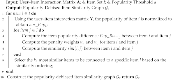
4.2. Feature Extraction of Items from Multiple Views

To explore and extract more comprehensive features from item nodes, graph encoders are built for the collaborative graph ${\mathcal{G}}_r$ and the popularity-debiased item similarity graph ${\mathcal{G}}_c$, respectively. The general form of the graph encoder structure is defined as follows:

$${\mathbf{E}}^{\left(l\right)}=\mathrm{H}({\mathbf{E}}^{(l-1)},\mathcal{G})$$

(6)

where $\mathrm{H}$ denotes the graph encoder for information aggregation, and $\mathcal{G}\in \{{\mathcal{G}}_r,{\mathcal{G}}_c\}$. We define ${\mathrm{H}}_r$ and ${\mathrm{H}}_c$ as graph encoders for graph ${\mathcal{G}}_r$ and graph ${\mathcal{G}}_c$, respectively. ${\mathbf{E}}^{\left(l\right)}$ and ${\mathbf{E}}^{(l-1)}$ are the node embedding in the $l^{th}$ and ${(l-1)}^{th}$ layers, respectively. When $l=0$, ${\mathbf{E}}^{\left(0\right)}$ represents the initial node embeddings.

Taking ${\mathrm{H}}_c$ as an example, the embedding of a specific node on ${\mathrm{H}}_c$ are denoted as ${\mathbf{e}}_i^{c\left(l\right)}$, in which the embedding of the $l^{th}$ layer is obtained by aggregating the layer ${(l-1)}^{th}$ embeddings of its neighboring node. The calculation is given by the following expression:

$${\mathbf{e}}_i^{c\left(l\right)}=\sum _{j\in N_i^c}\frac{1}{\sqrt{\mid N_i^c\mid }\sqrt{\mid N_j^c\mid }}{\mathbf{e}}_j^{c(l-1)}$$

(7)

where $N_i^c,N_j^c$ denote the sets of neighbors of item i and item j in the popularity-debiased item similarity graph ${\mathcal{G}}_c$, respectively. Then, through the stacking of information aggregation layers, the representations of each layer, denoted as ${\mathbf{e}}_i^{c\left(1\right)},\cdots ,{\mathbf{e}}_i^{c\left(l\right)}$, can be obtained by iteratively applying the aggregation Equation (7) to the initial embedding ${\mathbf{e}}_i^{c\left(0\right)}$. Finally, the embedding ${\mathbf{e}}_i^c$ for item i is obtained by weighted summation, which is calculated by

$${\mathbf{e}}_i^c=\sum _{l=0}^L{\alpha }_i{\mathbf{e}}_i^{c\left(l\right)}$$

(8)

where L denotes the total number of layers in the graph neural network information aggregation, and ${\alpha }_i$ represents the weight parameter of the embedding in the $l^{th}$ layer. In our experiments, we set ${\alpha }_i=1/(L+1)$.

Similarly, the collaborative embedding of item i, denoted as ${\mathbf{e}}_i^r$, can be obtained by ${\mathrm{H}}_r$ from the collaborative graph ${\mathcal{G}}_r$. In addition, ${\mathrm{H}}_r$ also serves the function of generating the user embedding ${\mathbf{e}}_u^r$ required for the recommendation task, where ${\mathbf{e}}_u^r,{\mathbf{e}}_i^r,{\mathbf{e}}_i^c\in {\mathbb{R}}^d$.

4.3. Constructing Self-Supervised Learning Tasks Based on Multiple Views

Embedding in different views focuses on containing information about different aspects of an item. Based on this, we learn self-supervised signals from others’ views to guide their own supervised information. Based on this idea, a self-supervised learning task between multiple views is constructed.

To generate extra self-supervised signals, we first create data augmentation views by applying edge dropout, a widely used graph data augmentation technique, to both graph ${\mathcal{G}}_r$ and graph ${\mathcal{G}}_c$. Specifically, during each iteration of the aggregation process in LightGCN, we randomly drop edges from graphs ${\mathcal{G}}_r$ and ${\mathcal{G}}_c$ with a certain probability $\rho$, thereby constructing data augmentation views and building an unlabeled sample set $\tilde{E}$. $\rho$ is a trainable hyperparameter. This makes it easier for the model to identify influential nodes in the augmentation view and reduce the sensitivity of the node representations to structural changes. The formulations are shown as

$$\begin{array}{cc}\hfill {\tilde{\mathcal{G}}}_r& =(N_r,{\mathbf{M}}_r\odot E_r)\hfill \end{array}$$

(9)

$$\begin{array}{cc}\hfill {\tilde{\mathcal{G}}}_c& =(N_c,{\mathbf{M}}_c\odot E_c)\hfill \end{array}$$

(10)

where $N_r,N_c$ and $E_r,E_c$ are the node set and edge set of ${\mathcal{G}}_r$ and ${\mathcal{G}}_c$, respectively. ${\mathbf{M}}_r\in {\{0,1\}}^{|E_r|}$ and ${\mathbf{M}}_c\in {\{0,1\}}^{|E_c|}$ are two maskers used to randomly drop out the edges of ${\mathcal{G}}_r$ and ${\mathcal{G}}_c$. ${\tilde{\mathcal{G}}}_r$ and ${\tilde{\mathcal{G}}}_c$ are the augmentation views, after performing the edge dropout operation on ${\mathcal{G}}_r$ and ${\mathcal{G}}_c$, respectively. Additionally, during the training process, the additional graph encoders are utilized to learn the embeddings of item nodes in the augmentation views. The learned item node embeddings are used as the unlabeled sample set $\tilde{E}$ for the initial graphs ${\mathcal{G}}_r$ and ${\mathcal{G}}_c$, reducing the sensitivity of node embedding learning to changes in graph structure.

We use ${\mathrm{H}}_c$ to learn the embedding ${\mathbf{e}}_i^c$ of item i from the popularity-debiased item similarity graph ${\mathcal{G}}_c$, which contains information about items that are similar to it after removing popularity bias. Obviously, ${\mathbf{e}}_i^c$ can provide supplementary information for the embedding of item i in collaborative graph ${\mathcal{G}}_r$. We can use it to predict the self-supervised signal for item i in the bias-removed item similarity graph ${\mathcal{G}}_c$, aiming to reduce the influence of item popularity in user–item interactions. The probability calculation formula $y_{i+}^r$ for the self-supervised signal in the popularity-debiased item similarity graph, using the node embeddings from the unlabeled sample set $\tilde{E}$ as follows:

$$y_{i+}^c=\sigma \left(\langle \tilde{\mathbf{e}},{\mathbf{e}}_i^c\rangle \right)$$

(11)

where $\langle ·\rangle$ indicates the inner product, and $\sigma$ is the Softmax function. To generate self-supervised signals that better align with the user’s true interests, we select the Top-K items with the highest ratings from the unlabeled sample set as the self-supervised signal $P_{i+}^r$ for the collaborative graph ${\mathcal{G}}_r$. The calculation is as follows:

$$P_{i+}^r=\{{\tilde{\mathbf{e}}}_k\mid k\in \mathrm{Top}\text{-}\mathrm{K}\left(y_{i+}^c\right),\tilde{E}\sim {\tilde{\mathcal{G}}}_r\}$$

(12)

Similarly, the self-supervised signal set $P_{i+}^c$ of the popularity-biased item similarity graph ${\mathcal{G}}_c$ is obtained by the following:

$$y_{i+}^r=\sigma \left(\langle \tilde{\mathbf{e}},{\mathbf{e}}_i^r\rangle \right)$$

(13)

$$P_{i+}^c=\{{\tilde{\mathbf{e}}}_k\mid k\in \mathrm{Top}\text{-}\mathrm{K}\left(y_{i+}^k\right),\tilde{E}\sim {\tilde{\mathcal{G}}}_c\}$$

(14)

Finally, the model maximizes the similarity between the embeddings of items in different views and their corresponding self-supervised signals, while minimizing the similarity between item embeddings and the unlabeled sample set. The unlabeled sample set is generated from the data augmentation views created by the views themselves. This is achieved by maximizing the mutual information between item node embeddings and self-supervised signals. Based on this, the self-supervised task loss function is constructed as follows:

$$\begin{array}{c}{L}_{ssl}=-\mathbb{E}{\displaystyle \sum _{v\in \{r,c\}}}\left[log\frac{{\displaystyle \sum _{p\in P_{i+}^v}}\psi ({\mathbf{e}}_i^v,{\tilde{\mathbf{e}}}_p)}{{\displaystyle \sum _{p\in P_{i+}^{\nu }}}\psi ({\mathbf{e}}_i^v,{\tilde{\mathbf{e}}}_p)+{\displaystyle \sum _{j\in I/P_{i+}^{\nu }}}\psi ({\mathbf{e}}_i^v,{\tilde{\mathbf{e}}}_j)}\right]\end{array}$$

(15)

$$\begin{array}{c}\psi ({\mathbf{e}}_i^v,{\tilde{\mathbf{e}}}_p)=\exp (\cos ({\mathbf{e}}_i^v·{\tilde{\mathbf{e}}}_p)/\tau )\end{array}$$

(16)

where $v\in \{r,c\}$ denotes the view set, r indicates the user–item interaction graph ${\mathcal{G}}_r$, and c indicates the popularity-debiased item similarity graph ${\mathcal{G}}_c$. ${\mathbf{e}}_i^v$ represents the item embedding of view v, $P_{i+}^v$ denotes the self-supervised signals set generated by the prediction of view v, ${\tilde{\mathbf{e}}}_p$ indicates the item embedding from the self-supervised signal set, and $j\in \mathit{I}/P_{i+}^v$ denotes the other item embedding in the unlabeled sample set.

4.4. Popularity-Aware Multitask Learning Strategy

The objective of PDGS is to predict the preference ratings of each user for candidate items. We employ the inner product to measure the similarity between users and candidate items, which serves as the calculation method for the prediction function, as shown

$${\widehat{y}}_{ui}={\mathbf{e}}_u^{rT}{\mathbf{e}}_i^r$$

(17)

During the model training process, the widely used BPR method will be influenced by item popularity when conducting negative sampling. Specifically, there is a higher probability of including long-tail items as negative samples in the model training, leading to a higher probability of the model learning user preferences towards popular items. This phenomenon makes popular items more and more popular, resulting in serious issues such as the Matthew Effect [30,31], echo chamber [32], and filter bubble [33,34]. Therefore, PDGS divides items into popular and long-tail sets using a popularity threshold $\alpha$. Then, we construct popularity-aware BPR optimization objectives from the perspectives of both popular and long-tail items. By integrating these two objectives, the final optimization function for the recommendation task is obtained as follows:

$$\begin{array}{c}\hfill L_r=-\sum _{(u,i,j)\in O_p}ln\sigma ({\widehat{y}}_{ui}-{\widehat{y}}_{uj})-\sum _{(u,i,j)\in O_{up}}ln\sigma ({\widehat{y}}_{ui}-{\widehat{y}}_{uj})\end{array}$$

(18)

where $\sigma$ is the Sigmoid function, $O_p=\left\{(u,i,j)\right|(u,i)\in O_p^{+},(u,j)\in O_p^{-}\}$ represents that both the positive sample i and the negative sample j are from the popular items set, while $O_{up}=\left\{(u,i,j)\right|(u,i)\in O_{up}^{+},(u,j)\in O_{up}^{-}\}$ represents that both the positive sample i and the negative sample j are from the long-tail items set.

Finally, to leverage self-supervised learning to enhance the model’s ability to improve recommendation diversity, PDGS adopts a joint strategy by simultaneously training the recommendation task and the self-supervised learning task. The model’s loss function is computed as follows:

$$L_{PDGS}=L_r+\beta L_{ssl}+\lambda {∥\Theta ∥}_2^2$$

(19)

where $L_r$ and $L_{ssl}$ are the loss functions of the recommendation task and the self-supervised task, respectively. $\beta$ and $\lambda$ are hyperparameters that control the scale of self-supervised learning and the strength of regularization, respectively. $\Theta =\{{\mathbf{e}}_u^r,{\mathbf{e}}_i^r,{\mathbf{e}}_i^c\}$ represents the parameters to be learned by the model.

4.5. Complexity of PDGS

The time complexity of PDGS mainly comes from the graph encoder, self-supervised signal prediction, and multiview self-supervised learning. Firstly, the time complexity of the graph encoder can be represented as $|\mathcal{G}|d$, where $|\mathcal{G}|$ represents the scale of the graph structure learned by the graph encoder, and d represents the embedding dimension of entities in the model. Since PDGS consists of two graph encoders used for learning the entity embeddings of the user–item interaction graph ${\mathcal{G}}_r$ and the popularity-debiased item similarity graph ${\mathcal{G}}_c$, the time complexity from the graph encoder is denoted as $((|{\mathcal{G}}_r|+|{\mathcal{G}}_c|+|\tilde{\mathcal{G}}|)d)$. Secondly, the time complexity of self-supervised signal prediction is represented as $\mathcal{O}\left(\left(x\log \right(\mathrm{K}\left)\right)\right)$, where x denotes the number of randomly selected unlabeled samples in each training batch, and $\mathrm{K}$ represents the number of self-supervised signals to be predicted from the unlabeled sample set. Finally, as the model uses a shared graph encoder for the joint optimization of self-supervised learning and the recommendation task, the time complexity of the multiview self-supervised learning task mainly comes from the self-supervised signals between views and the contrastive learning of item entities. This part of the time complexity can be represented as $\mathcal{O}\left(xd\right)$.

5. Experiment

In this section, we conduct extensive experiments on three real datasets to evaluate the performance of our proposed model. Our experiment aims to answer the following research questions:

RQ1: Does the model outperform existing baseline methods?

RQ2: How can the different components in our framework improve performance?

RQ3: How do different hyperparameter settings affect recommendation performance?

5.1. Experiment Setup

5.1.1. Dataset Description

To validate the effectiveness of the model, the model performance is evaluated on three different datasets from diverse domains with varying scales and sparsity. MovieLens-1M is a movie recommendation dataset that includes user ratings for movies on a scale of 1–5. Book-Crossing is a book recommendation dataset that includes user ratings for books on a scale of 1–10. Although both of these datasets are explicit feedback datasets, we intentionally chose them to study the performance of learning from implicit feedback. To achieve this, we transform them into implicit data, where each item is labeled as 0 or 1, indicating whether the user has rated the item or not. Last-FM is a music recommendation dataset that contains users’ one-year listening history on the Last.fm website.

Table 1. The statistics of the Datasets.

	Users	Item	Interaction	Sparsity
MovieLens-1M	5986	2347	298,856	97.8728%
Last-FM	1872	3846	42,346	99.4118%
Book-Crossing	17,860	14,910	139,746	99.9475%

summarizes the statistical information of these datasets.

5.1.2. Evaluation Protocol

To evaluate the accuracy of the model, common metrics such as Recall and Normalized Discounted Cumulative Gain (NDCG) are used. Additionally, to verify the impact of reducing the popularity bias on the model, evaluation metrics that measure the diversity of the model’s recommendation results are used: Coverage and Novelty.

Coverage (Cov@K) [35] is used to measure the proportion of items covered in the item space by the recommendation results. Its expression is given by

$$\mathrm{Cov}@\mathrm{K}=\frac{|{\displaystyle \bigcup _{u\in U}}{R}_u@\mathrm{K}|}{\left|I\right|}$$

(20)

where U is the user set, I is the item set, and $R_u@\mathrm{K}$ denotes the $\mathrm{Top}$-$\mathrm{K}$ recommendation list of user u.

Novelty (Tail@K) [36] is used to measure the percentage of long-tail items in the $\mathrm{Top}$-$\mathrm{K}$ recommendation list for all users, and its expression is shown as follows

$$\mathrm{Tail}@\mathrm{K}=\frac{1}{\left|U\right|}\sum _{u\in U}\frac{\left|R_u@\mathrm{K}\cap I_{up}\right|}{\mathrm{K}}$$

(21)

where U is the user set, $I_{up}$ is the long-tail item set, and $R_u@\mathrm{K}$ denotes the $\mathrm{Top}$-$\mathrm{K}$ recommendation list of user u.

5.1.3. Baselines

To validate the effectiveness of the proposed model PDGS, we compare PDGS with the following baselines in our experiments:

-

$\mathbf{NeuMF}$ [37]: It combines Generalized Matrix Factorization and MultiLayer Perceptron to extract low-dimensional and high-dimensional features simultaneously.

-

$\mathbf{NGCF}$ [38]: It utilizes graph neural networks to model high-order connectivity information and capture collaborative information between nodes.

-

$\mathbf{LightGCN}$ [29]: It designs a lightweight graph convolution operation that simplifies model design to a large extent, which includes the most important components in GCN for recommendation.

-

$\mathbf{SGL}$ [39]: It designs multiple data augmentation methods to construct a comparative learning task to learn node representations with the help of mutual information maximization idea.

-

$\mathbf{MCCLK}$ [27]: It generates global-, local-, and semantic-level contrastive views, constructs contrastive learning tasks, and explores comprehensive graph features and structural information in a self-supervised manner.

5.2. Performance Comparison with Baselines

For the proposed model PDGS, we use the Adam optimizer to learn the model. For each dataset, 80% is randomly selected as the training set, and the remaining 20% is divided equally into the validation set and the test set. We use 5-fold cross-validation with Recall@20 as the validation metric. The detailed hyperparameters settings of the models can be found in

Table 2. Hyperparameter Settings for Three Datasets.

	$\mathit{\alpha }$	${\mathit{k}}_{\mathit{c}}$	d	$\mathbf{K}$	$\mathit{\beta }$	$\mathit{\rho }$
MovieLens-1M	0.049	100	50	15	0.01	0.3
Last-FM	0.017	100	50	30	0.002	0.3
Book-Crossing	0.002	100	50	40	0.005	0.3

.

Figure 2 illustrates the recommendation performance of the comparative models on Top-10 and Top-20 recommendation tasks in terms of four evaluation protocols. Overall, we proposed PDGS model outperforms all baselines in terms of the evaluation metrics across all three datasets. The detailed improvements in model performance are shown in

Table 3. PDGS performance improvement percentage.

Dataset	@10				@20
	Recall	NDCG	Cov	Tail	Recall	NDCG	Cov	Tail
Movie-Lens	1.5563%	0.0741%	7.8595%	4.0219%	1.4689%	1.4233%	0.6923%	5.0113%
Last-FM	2.5941%	3.1316%	6.1177%	7.6510%	1.0083%	2.0859%	2.3567%	5.3212%
Book-Crossing	0.7866%	4.5612%	7.4062%	11.4480%	1.2048%	0.2484%	0.5781%	1.6671%

.

(1)

It is intuitively clear from Figure 2 that our proposed model PDGS outperforms the comparison models both in terms of accuracy and novelty recommendation. Table 3 digitally demonstrates the performance improvement of PDGS on all evaluation metrics. It illustrates that the model PDGS can effectively improve the problem of insufficient diversity of recommended items in the existing models and increase the recommendation ratio of long-tail items. It can fully explore the value of long-tail items, enhance user engagement, and generate more revenue for businesses.

(2)

In both Top-10 and Top-20 recommendations, the PDGS model achieves optimal results in terms of recommendation accuracy compared with all baselines, indicating that the PDGS algorithm does not trade off the loss of accuracy for the diversity of recommended items. From a practical perspective, solely improving the diversity of item recommendations without considering that recommendation accuracy loses the significance of personalized recommendation. Our proposed PDGS model can effectively balance the dilemma between recommendation accuracy and diversity, fully explore the uninteracted items related to users’ interests, and improve the performance of the recommendation model as a whole.

(3)

Compared with the self-supervised recommendation models SGL and MCCLK, our proposed PDGS achieves optimal performance in recommendation diversity evaluation metrics. The method of data augmentation of the user–item interaction graph from the perspective of popularity debiased item similarity is illustrated, which takes into account user preferences while eliminating the influence of popularity bias, making the generated self-supervised signals more in line with the real situation and allowing more long-tail items to be covered in the recommendation lists, thus effectively reducing the problem of popularity bias that exists in the original user–item historical interaction dataset.

5.3. Ablation Study of PDGS

To further validate the effectiveness of the model components in improving recommendation performance, we designed two variants of PDGS. One is to replace the popularity-debiased item graph with an item similarity graph to participate in contrastive learning with the collaborative graph, denoted as PDGS-NC. The other is to replace the loss function designed for popular items and long-tail items with the traditional BPR loss function, denoted as PDGS-BPR. The hyperparameter settings of the variant models remain consistent with PDGS. The results of the ablation experiments on three datasets are shown in

Table 4. Performance compared with model variants of PDGS.

Dataset	Metric	PDGS-NC	PDGS-BPR	PDGS
MovieLens-1M	Recall@10	24.477	25.214	25.123
	NDCG@10	22.243	23.291	22.948
	Cov@10	58.126	56.526	60.740
	Tail@10	58.473	53.654	61.116
Last-FM	Recall@10	28.485	29.141	28.871
	NDCG@10	21.175	21.803	21.604
	Cov@10	64.663	62.351	68.586
	Tail@10	21.435	20.595	23.075
Book-Crossing	Recall@10	9.155	9.752	9.610
	NDCG@10	5.567	6.416	6.327
	Cov@10	65.415	62.247	69.828
	Tail@10	27.970	26.357	30.432

, with the best performance indicated in bold.

From the experimental results in Table 4, it can be observed that PDGS-NC exhibits a certain decrease in both the Cov@10 and Tail@10 evaluation metrics compared with PDGS. This indicates that the data-enhanced view learning without adding the popularity restriction in the self-supervised learning task will lead the model to reduce attention to long-tail items. Consequently, the representation learning of long-tail items and the generation of self-supervised signals that are closer to real samples are restricted, resulting in poorer performance in terms of coverage (Cov@10) and novelty (Tail@10).

Furthermore, comparing PDGS and PDGS-BPR, when the recommendation task loss function is changed to the traditional BPR loss function, there is a certain improvement in accuracy metrics (Recall@10 and NDCG@10), but diversity metrics (Cov@10 and Tail@10) experience a significant decrease. This is because the BPR loss function tends to focus on popular items that have been interacted with more frequently in the user’s history. The model learns more about the items that the user has previously engaged with, leading to improved recommendation accuracy. However, due to the interference of popularity bias, it results in lower coverage (Cov@10) and novelty (Tail@10). From the comparative results, it can be observed that directly using the BPR loss function exacerbates the influence of popularity bias. On the other hand, the recommendation task loss function that considers both popular and long-tail items alleviates this issue by balancing the impact of popularity and users’ true interests in item selection.

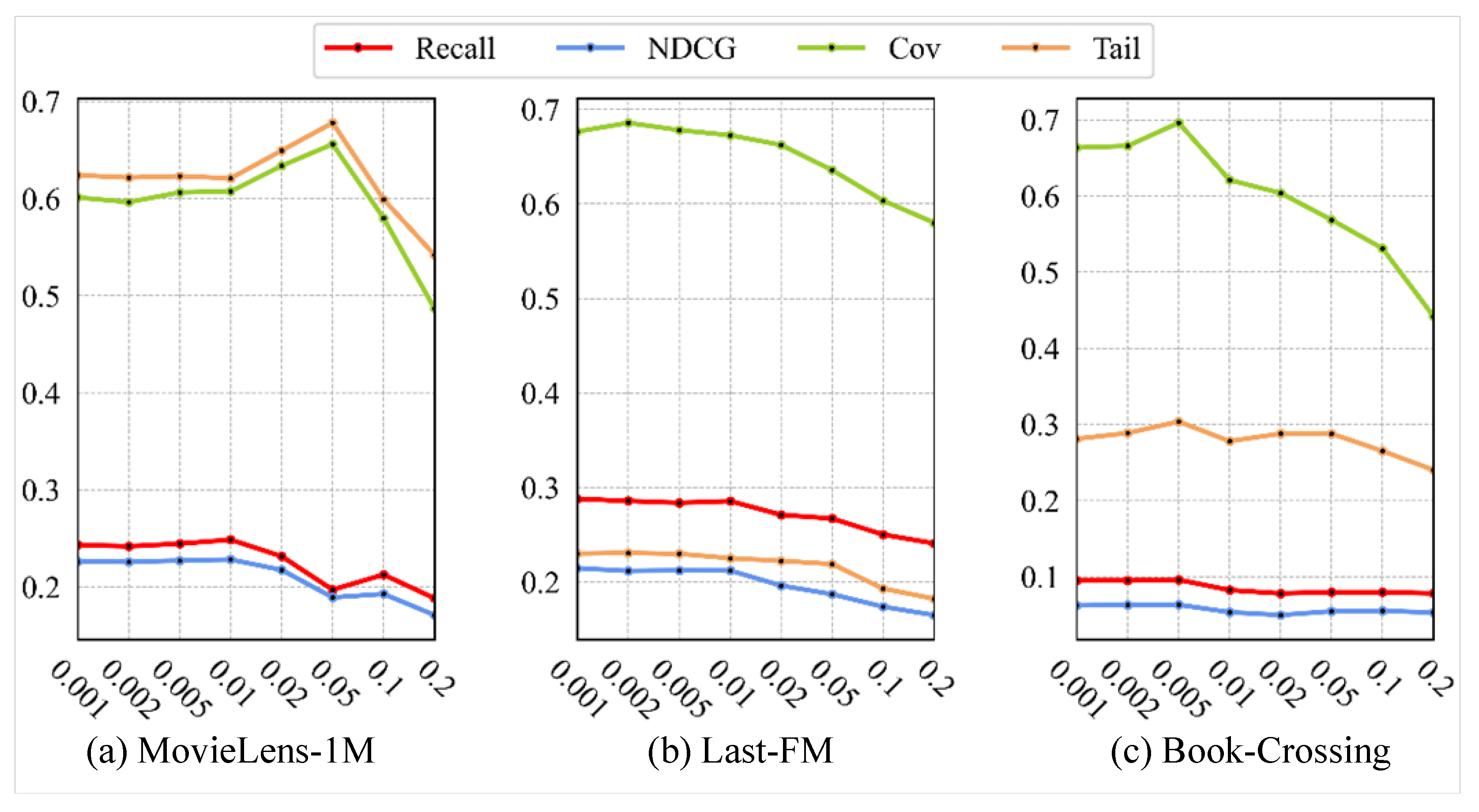
5.4. Impact of the Number of Hyperparameters

To verify the effect of hyperparameters on model performance, we set specific ranges for different hyperparameters, the scale weight coefficient $\beta \in$ [0.001, 0.002, 0.005, 0.01, 0.02, 0.05, 0.1, 0.2] for self-supervised learning, the quantity of self-supervised signals $\mathrm{K}\in [1,5,10,15,20,30,40,50,100]$, and the number layers of the graph neural network encoder $L\in [1,2,3,4,5]$, respectively, and retrain the model on the Top-10 recommendation task. The results are shown in Figure 3, Figure 4 and Figure 5.

In order to investigate the effect of the $\beta$ value on model performance, we fixed the other two parameters and set $L=2$ on the three datasets, and the number of self-supervised signals on the three datasets is set to K = 15, 30, and 40, respectively. From Figure 3, it can be seen that as the value of $\beta$ increases, and the indicators for measuring model accuracy, Recall, and NDCG show relatively minor fluctuations. However, when $\beta >0.01$, the model’s performance exhibits a decreasing trend on both the MovieLens-1M and Last-FM datasets. On the Book-Crossing dataset, the decreasing trend begins at $\beta >0.005$. Meanwhile, as the value of $\beta$ gradually increases, the metrics evaluating recommendation diversity, Cov and Tail, initially increase and then decrease across all three datasets. Overall, when the value of $\beta$ is small, the self-supervised task serving as an auxiliary task improves recommendation diversity without significantly affecting the recommendation accuracy. However, as the value of $\beta$ continues to increase, the model’s performance is affected to varying degrees in terms of accuracy and diversity. Taking all factors into consideration, we set the self-supervised learning weight coefficient $\beta$ as 0.01, 0.002, and 0.005 for the MovieLens-1M, Last-FM, and BookCrossing datasets, respectively.

In order to explore the effect of the number of self-supervised signals K on model performance, we set $L=2$ for all three datasets, with $\beta$ values set as 0.01, 0.002, and 0.005, respectively. From Figure 4, it can be observed that as K increases, the performance metrics evaluating recommendation accuracy, Recall, and NDCG exhibit an initially increasing and then decreasing trend on the MovieLens-1M and Last-FM datasets. However, the change is minimal on the BookCrossing dataset, indicating that the variation in K has little impact on this dataset. Additionally, the metrics evaluating recommendation diversity, Cov and Tail, show varying degrees of improvement across all three datasets, suggesting that higher values of K positively encourage diverse recommendations. A reasonable value of K can effectively alleviate the issue of data sparsity and facilitate better learning of user and item embeddings by the model. However, it should be noted that self-supervised signals are predicted based on confidence, and as K increases, more noise is introduced, leading to a decrease in the model’s recommendation accuracy. Taking all of these factors into consideration, we set the number of self-supervised signals K to 100 for all three datasets in PDGS.

To investigate the effect of the parameter L on the model, we fixed $\beta$ and K on three datasets as $\beta =0.01,0.002,0.005$ and $K=15,30,40$. From Figure 5, it can be observed that as L increases from 1 to 2, the evaluation metrics for recommendation accuracy, Recall, and NDCG show a significant improvement on the MovieLens-1M and Last-FM datasets, while they remain relatively unchanged on the Book-Crossing dataset. However, as L continues to increase from 2 to 5, Recall and NDCG exhibit different degrees of decline on all datasets. This indicates that a large number of network layers increases the complexity of the model, causing the learned node representations to become more homogeneous, which leads to a decrease in model performance. Similarly, when L increases from 1 to 2, the metrics evaluating recommendation diversity, Cov and Tail, show a noticeable improvement across all three datasets. However, when $L>2$, the growth in the metrics evaluating recommendation diversity becomes less significant. Balancing recommendation accuracy and diversity is crucial in recommendation systems. Taking all factors into consideration, we set the number of layers in the graph encoder $L=2$ in the PDGS model to encourage the discovery of more long-tail items among the unobserved items for users.

6. Conclusions

In view of the fact that data sparseness and long-tail features in recommendation systems lead to insufficient diversity of recommended items, which negatively impacts users’ satisfaction and merchants’ revenue, we proposed a popularity-debiased graph self-supervised recommendation model PDGS. For popular items and long-tail items, we designed corresponding penalty functions, constructed an item similarity graph that removes the popularity bias, and conducted comparative learning with the collaboration graph to alleviate the sparsity of the data. In addition, we designed optimization functions for popular items and long-tail items, respectively, and built a multitask learning strategy to generate an end-to-end training model. We verified the superiority of the model through extensive comparative experiments and ablation experiments on different datasets. In real life, popular items may also be favored by most people because of their good quality. Therefore, in future work, considering the contribution of popular items to recommendation performance in different scenarios will be a direction worthy of research.

References

1. Lian, J.; Zhou, X.; Zhang, F.; Chen, Z.; Xie, X.; Sun, G. xdeepfm: Combining explicit and implicit feature interactions for recommender systems. In Proceedings of the 24th ACM SIGKDD International Conference on Knowledge Discovery & Data Mining, London, UK, 19–23 August 2018; pp. 1754–1763. [Google Scholar]
2. Lin, Z.; Tian, C.; Hou, Y.; Zhao, W.X. Improving graph collaborative filtering with neighborhood-enriched contrastive learning. In Proceedings of the ACM Web Conference 2022, Lyon, France, 25–29 April 2022; pp. 2320–2329. [Google Scholar]
3. Abdollahpouri, H. Popularity bias in ranking and recommendation. In Proceedings of the 2019 AAAI/ACM Conference on AI, Ethics, and Society, Honolulu, HI, USA, 27–28 January 2019; pp. 529–530. [Google Scholar]
4. Saito, Y.; Yaginuma, S.; Nishino, Y.; Sakata, H.; Nakata, K. Unbiased recommender learning from missing-not-at-random implicit feedback. In Proceedings of the 13th International Conference on Web Search and Data Mining, Houston, TX, USA, 3–7 February 2020; pp. 501–509. [Google Scholar]
5. Chen, J.; Dong, H.; Wang, X.; Feng, F.; Wang, M.; He, X. Bias and debias in recommender system: A survey and future directions. ACM Trans. Inf. Syst. 2023, 41, 1–39. [Google Scholar] [CrossRef]
6. Yang, L.; Cui, Y.; Xuan, Y.; Wang, C.; Belongie, S.; Estrin, D. Unbiased offline recommender evaluation for missing-not-at-random implicit feedback. In Proceedings of the 12th ACM Conference on Recommender Systems, Vancouver, BC, Canada, 2–7 October 2018; pp. 279–287. [Google Scholar]
7. Zhu, Z.; He, Y.; Zhao, X.; Zhang, Y.; Wang, J.; Caverlee, J. Popularity-opportunity bias in collaborative filtering. In Proceedings of the 14th ACM International Conference on Web Search and Data Mining, Jerusalem, Israel, 8–12 March 2021; pp. 85–93. [Google Scholar]
8. Bonner, S.; Vasile, F. Causal embeddings for recommendation. In Proceedings of the 12th ACM Conference on Recommender Systems, Vancouver, BC, Canada, 2–7 October 2018; pp. 104–112. [Google Scholar]
9. Elahi, M.; Kholgh, D.K.; Kiarostami, M.S.; Saghari, S.; Rad, S.P.; Tkalčič, M. Investigating the impact of recommender systems on user-based and item-based popularity bias. Inf. Process. Manag. 2021, 58, 102655. [Google Scholar] [CrossRef]
10. Wei, T.; Feng, F.; Chen, J.; Wu, Z.; Yi, J.; He, X. Model-agnostic counterfactual reasoning for eliminating popularity bias in recommender system. In Proceedings of the 27th ACM SIGKDD Conference on Knowledge Discovery & Data Mining, Singapore, 14–18 August 2021; pp. 1791–1800. [Google Scholar]
11. Zhang, Y.; Feng, F.; He, X.; Wei, T.; Song, C.; Ling, G.; Zhang, Y. Causal intervention for leveraging popularity bias in recommendation. In Proceedings of the 44th International ACM SIGIR Conference on Research and Development in Information Retrieval, Virtual Event, 11–15 July 2021; pp. 11–20. [Google Scholar]
12. Fu, Z.; Xian, Y.; Geng, S.; De Melo, G.; Zhang, Y. Popcorn: Human-in-the-loop popularity debiasing in conversational recommender systems. In Proceedings of the 30th ACM International Conference on Information & Knowledge Management, Virtual Event, 1–5 November 2021; pp. 494–503. [Google Scholar]
13. Abdollahpouri, H.; Mansoury, M.; Burke, R.; Mobasher, B. The connection between popularity bias, calibration, and fairness in recommendation. In Proceedings of the 14th ACM Conference on Recommender Systems, Virtual, 22–26 September 2020; pp. 726–731. [Google Scholar]
14. Rhee, W.; Cho, S.M.; Suh, B. Countering Popularity Bias by Regularizing Score Differences. In Proceedings of the 16th ACM Conference on Recommender Systems, Seattle, WA, USA, 18–23 September 2022; pp. 145–155. [Google Scholar]
15. Zhao, W.; Tang, D.; Chen, X.; Lv, D.; Ou, D.; Li, B.; Jiang, P.; Gai, K. Disentangled Causal Embedding With Contrastive Learning For Recommender System. arXiv 2023, arXiv:2302.03248. [Google Scholar]
16. Zhanga, X.; Sua, K.; Qiana, F.; Zhangc, Y.; Zhanga, K. Collaborative Filtering Algorithm Based on Item Popularity and Dynamic Changes of Interest. In Modern Management Based on Big Data III; IOS Press: Amsterdam, The Netherlands, 2022; pp. 132–140. [Google Scholar]
17. Yang, S.; Cai, B.; Cai, T.; Song, X.; Jiang, J.; Li, B.; Li, J. Robust cross-network node classification via constrained graph mutual information. Knowl.-Based Syst. 2022, 257, 109852. [Google Scholar] [CrossRef]
18. Hoang, T.; Do, T.T.; Nguyen, T.V.; Cheung, N.M. Multimodal mutual information maximization: A novel approach for unsupervised deep cross-modal hashing. IEEE Trans. Neural Netw. Learn. Syst. 2022, 34, 6289–6302. [Google Scholar] [CrossRef] [PubMed]
19. Linsker, R. Self-organization in a perceptual network. Computer 1988, 21, 105–117. [Google Scholar] [CrossRef]
20. Fan, J.; Yu, Y.; Huang, L.; Wang, Z. GraphDPI: Partial label disambiguation by graph representation learning via mutual information maximization. Pattern Recognit. 2023, 134, 109133. [Google Scholar] [CrossRef]
21. Sanghi, A. Info3d: Representation learning on 3d objects using mutual information maximization and contrastive learning. In Proceedings of the Computer Vision–ECCV 2020: 16th European Conference, Glasgow, UK, 23–28 August 2020; Proceedings, Part XXIX 16. Springer: Cham, Switzerland, 2020; pp. 626–642. [Google Scholar]
22. Mohamed, A.; Lee, H.y.; Borgholt, L.; Havtorn, J.D.; Edin, J.; Igel, C.; Kirchhoff, K.; Li, S.W.; Livescu, K.; Maaløe, L.; et al. Self-supervised speech representation learning: A review. IEEE J. Sel. Top. Signal Process. 2022, 16, 1179–1210. [Google Scholar] [CrossRef]
23. Hsu, W.N.; Bolte, B.; Tsai, Y.H.H.; Lakhotia, K.; Salakhutdinov, R.; Mohamed, A. Hubert: Self-supervised speech representation learning by masked prediction of hidden units. IEEE/ACM Trans. Audio Speech Lang. Process. 2021, 29, 3451–3460. [Google Scholar] [CrossRef]
24. Han, W.; Chen, H.; Poria, S. Improving Multimodal Fusion with Hierarchical Mutual Information Maximization for Multimodal Sentiment Analysis. In Proceedings of the 2021 Conference on Empirical Methods in Natural Language Processing, Virtual Event, 7–11 November 2021; pp. 9180–9192. [Google Scholar]
25. Zhou, K.; Wang, H.; Zhao, W.X.; Zhu, Y.; Wang, S.; Zhang, F.; Wang, Z.; Wen, J.R. S3-rec: Self-supervised learning for sequential recommendation with mutual information maximization. In Proceedings of the 29th ACM International Conference on Information & Knowledge Management, Virtual Event, 19–23 October 2020; pp. 1893–1902. [Google Scholar]
26. Ma, J.; Zhou, C.; Yang, H.; Cui, P.; Wang, X.; Zhu, W. Disentangled self-supervision in sequential recommenders. In Proceedings of the 26th ACM SIGKDD International Conference on Knowledge Discovery & Data Mining, Virtual Event, 6–10 July 2020; pp. 483–491. [Google Scholar]
27. Zou, D.; Wei, W.; Mao, X.L.; Wang, Z.; Qiu, M.; Zhu, F.; Cao, X. Multi-level cross-view contrastive learning for knowledge-aware recommender system. In Proceedings of the 45th International ACM SIGIR Conference on Research and Development in Information Retrieval, Madrid, Spain, 11–15 July 2022; pp. 1358–1368. [Google Scholar]
28. Ji, Y.; Sun, A.; Zhang, J.; Li, C. A re-visit of the popularity baseline in recommender systems. In Proceedings of the 43rd International ACM SIGIR Conference on Research and Development in Information Retrieval, Virtual Event, 25–30 July 2020; pp. 1749–1752. [Google Scholar]
29. He, X.; Deng, K.; Wang, X.; Li, Y.; Zhang, Y.; Wang, M. Lightgcn: Simplifying and powering graph convolution network for recommendation. In Proceedings of the 43rd International ACM SIGIR Conference on Research and Development in Information Retrieval, Xi’an, China, 25–30 July 2020; pp. 639–648. [Google Scholar]
30. Perc, M. The Matthew effect in empirical data. J. R. Soc. Interface 2014, 11, 20140378. [Google Scholar] [CrossRef] [PubMed]
31. Steck, H. Calibrated recommendations. In Proceedings of the 12th ACM Conference on Recommender Systems, Vancouver, BC, Canada, 2–7 October 2018; pp. 154–162. [Google Scholar]
32. Ge, Y.; Zhao, S.; Zhou, H.; Pei, C.; Sun, F.; Ou, W.; Zhang, Y. Understanding echo chambers in e-commerce recommender systems. In Proceedings of the 43rd international ACM SIGIR Conference on Research and Development in Information Retrieval, Xi’an, China, 25–30 July 2020; pp. 2261–2270. [Google Scholar]
33. Mehrotra, R.; McInerney, J.; Bouchard, H.; Lalmas, M.; Diaz, F. Towards a fair marketplace: Counterfactual evaluation of the trade-off between relevance, fairness & satisfaction in recommendation systems. In Proceedings of the 27th ACM International Conference on Information and Knowledge Management, Torino, Italy, 22–26 October 2018; pp. 2243–2251. [Google Scholar]
34. Cañamares, R.; Castells, P. Should I follow the crowd? A probabilistic analysis of the effectiveness of popularity in recommender systems. In Proceedings of the The 41st International ACM SIGIR Conference on Research & Development in Information Retrieval, Ann Arbor, MI, USA, 8–12 July 2018; pp. 415–424. [Google Scholar]
35. Liu, S.; Zheng, Y. Long-tail session-based recommendation. In Proceedings of the 14th ACM Conference on Recommender Systems, Virtual Event, 22–26 September 2020; pp. 509–514. [Google Scholar]
36. Zolaktaf, Z.; Babanezhad, R.; Pottinger, R. A generic top-n recommendation framework for trading-off accuracy, novelty, and coverage. In Proceedings of the 2018 IEEE 34th International Conference on Data Engineering (ICDE), Paris, France, 16–19 April 2018; pp. 149–160. [Google Scholar]
37. He, X.; Liao, L.; Zhang, H.; Nie, L.; Hu, X.; Chua, T.S. Neural collaborative filtering. In Proceedings of the 26th International Conference on World Wide Web, Perth, Australia, 3–7 April 2017; pp. 173–182. [Google Scholar]
38. Wang, X.; He, X.; Wang, M.; Feng, F.; Chua, T.S. Neural graph collaborative filtering. In Proceedings of the 42nd international ACM SIGIR Conference on Research and Development in Information Retrieval, Paris, France, 21–25 July 2019; pp. 165–174. [Google Scholar]
39. Wu, J.; Wang, X.; Feng, F.; He, X.; Chen, L.; Lian, J.; Xie, X. Self-supervised graph learning for recommendation. In Proceedings of the 44th international ACM SIGIR Conference on Research and Development in Information Retrieval, Virtual Event, 11–15 July 2021; pp. 726–735. [Google Scholar]
Figure 1. The overall framework of PDGS.
Electronics 13 00677 g001
Figure 2. Comparison of the performance of different models: (a1a4) ML represents MovieLens-1M; (b1b4) LF represents Last-FM; (c1c4) BC represents Book-Crossing.
Electronics 13 00677 g002
Figure 3. Performance of PDGS with reference to the number of the  β .
Electronics 13 00677 g003
Figure 4. Performance of PDGS with reference to the number of the K.
Electronics 13 00677 g004
Figure 5. Performance of PDGS with reference to the number of L.
Electronics 13 00677 g005