Abstract
Neural network pruning has been widely studied for model compression and acceleration, to facilitate model deployment in resource-limited scenarios. Conventional methods either require domain knowledge to manually design the pruned model architecture and pruning algorithm, or AutoML-based methods to search the pruned model architecture but still prune all layers with a single pruning algorithm. However, many pruning algorithms have been proposed and they all differ regarding the importance they attribute to the criterion of filters. Therefore, we propose a hybrid search method, searching for the pruned model architecture and the pruning algorithm at the same time, which automatically finds the pruning ratio and pruning algorithm for each convolution layer. Moreover, to be more efficient, we divide the search process into two phases. Firstly, we search in a huge space with adaptive batch normalization, which is a fast but relatively inaccurate model evaluation method; secondly, we search based on the previous results and evaluate models by fine-tuning, which is more accurate. Therefore, our proposed hybrid search method is efficient, and achieves a clear improvement in performance compared to current state-of-the-art methods, including AMC, MetaPruning, and ABCPruner. For example, when pruning MobileNet, we achieve a test accuracy on ImageNet with only 49 M FLOPs, which is higher than MetaPruning.
1. Introduction
Deep neural networks (DNNs) have made significant progress in various computer vision tasks (e.g., image classification [1,2,3], object detection [4,5], image segmentation [6,7]), and other applications [8,9,10,11,12,13]. However, the high computational cost makes it difficult to deploy them in edge devices (e.g., robots, self-driving cars, and drones). To this end, network compression and acceleration methods, which include pruning [14,15,16,17,18,19,20,21,22], quantization [15,23,24,25,26]), distillation [27,28,29,30,31], and black box optimization [32,33], have been widely investigated. Among these methods, network pruning has received particular attention due to its high accuracy and compression/acceleration rate. However, conventional structured pruning methods [14,18,20,34] need to manually design the pruned model architecture before pruning filters or channels according to the specific importance criterion (e.g., norm [14], geometric median [20], and rank of the feature maps [22]). To find an optimal pruned model architecture, some AutoML-based methods [35,36] have been proposed. AMC [19] optimizes the objective by deep reinforcement learning under constraints such as model parameters or FLOPs. However, AMC [19] evaluates the candidate model with the least squares method [34], which is slow and inaccurate. EagleEye [37] evaluates the candidate model with adaptive batch normalization(adaptive-BN), which is efficient but relatively inaccurate. Moreover, previous AutoML-based pruning methods often prune the filters in all convolution layers with the same importance criterion, which is inappropriate because input feature maps and filter weights of different layers have different distributions.
In this work, we reference foundational pruning algorithms to construct our search space for network optimization. Ref. [14] introduces a technique for efficient model pruning, ref. [20] proposes a method for reducing CNN computational complexity, and ref. [22] develops HRank for filter pruning based on hierarchical ranks. These methods inform our approach to identifying effective pruning strategies, enabling us to explore a broad range of options for enhancing network architecture. With such a search space, we can find the specific pruning algorithm for each convolution layer to be pruned. Furthermore, we can search the pruned model architecture and pruning algorithms simultaneously, as illustrated in Figure 1.
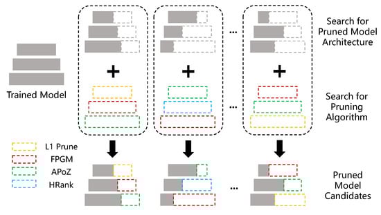
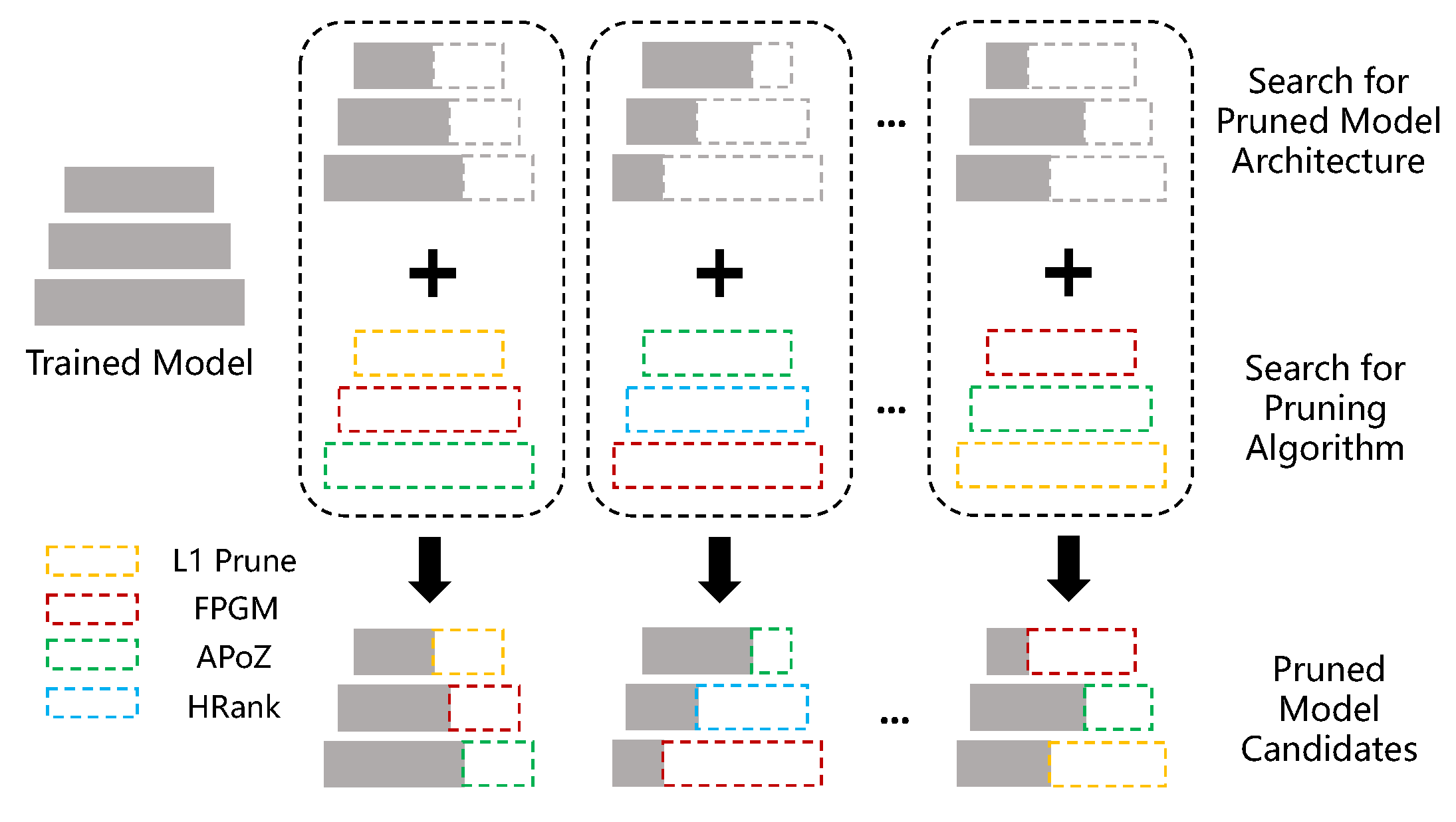
Figure 1.
The image illustrates a method for optimizing a neural network through a dual-search approach. The method simultaneously searches for the ideal pruning ratio and the most suitable pruning algorithm for each layer of a trained model. It evaluates various combinations of pruning strategies on different layers, leading to multiple pruned model candidates. The goal is to automate the selection process to achieve an efficient balance between model size, speed, and accuracy.
However, the accurate model evaluation method (e.g., fine-tuning few epochs) is too slow, and the efficient method (e.g., adaptive-BN) is relatively inaccurate. Thus, we need to firstly search in a huge space with an efficient method, then proceed to the next search phase based on the results of the first search phase, and evaluate the candidates with a more accurate method.
In this paper, we propose a fast hybrid search method to search the pruned model architecture and pruning algorithm simultaneously (Figure 1). Specifically, we build a search space of pruning algorithm based on previous works, which includes pruning [14], FPGM [20], HRank [22], and APoZ [38]. Furthermore, we encode the pruning ratio of all layers into a vector s, and the choice of pruning algorithm of all layers into a vector c, and then search for the pruned model architecture and pruning algorithm simultaneously. To be more efficient, we separate the search process into two phases and switch the model evaluation method from the efficient method to the more accurate method in the later phase, which efficiently handles the aforementioned problems. In the first phase, we explore the search space with the evolution algorithm, during which the pre-trained model will be pruned with the candidate pruning ratio s and pruning algorithm c. If the pruned model has more FLOPs than the given target, it will be discarded; otherwise, the pruned model will be evaluated by adaptive-BN [37], which is fast but relatively inaccurate. In the second phase, we select the top-K candidates with the highest accuracy in the first search phase into a set to form a new search space. Then, we evaluate each candidate in the set by fine-tuning the pruned model for few epochs, which is slower but more accurate. All the candidates in will be evaluated. The overall workflow of our proposed hybrid search method is illustrated in Figure 2.
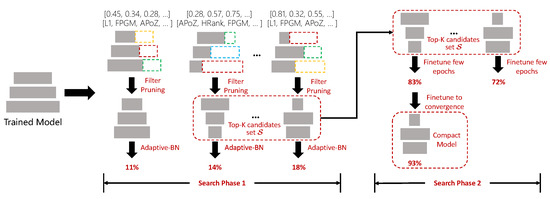
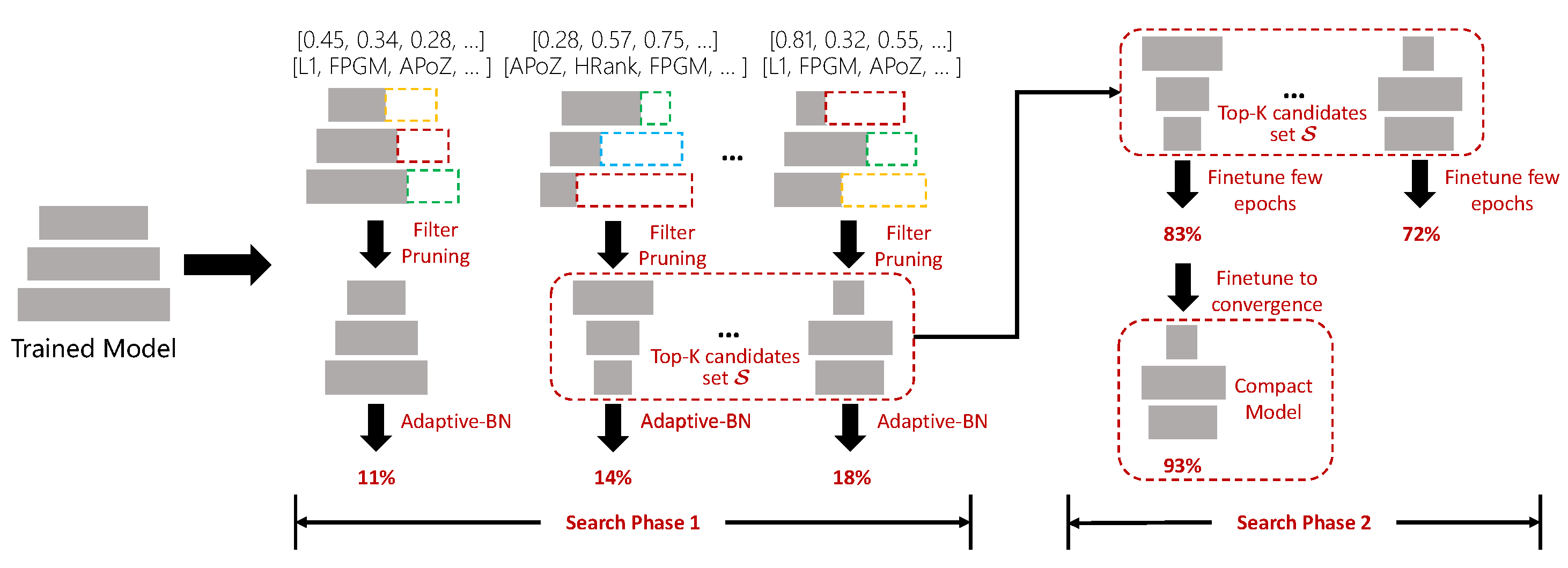
Figure 2.
Workflow of our proposed fast hybrid search method. We search for the pruned model architecture and pruning algorithms simultaneously and divide the search process into two phases for efficiency. In the first search phase, we use adaptive-BN to evaluate candidate models and the Top-K candidates with the highest validation accuracy are inserted into a set ; then, in the second phase, we evaluate each candidate in by fine-tuning a few epochs; finally, the best candidate model in is fine-tuned to convergence.
Quantitatively, we compress VGG-16 [1] to FLOPs with only a drop in accuracy on CIFAR-10. In addition, we can leverage the proposed hybrid search to compress MobileNet [39] to only 49 M FLOPs with test accuracy, and MobileNetV2 [40] to 148 M FLOPs with test accuracy on ImageNet [41].
The contributions of this work are summarized as follows:
- We firstly propose a hybrid search method for automatic filter pruning, which searches the pruned model architecture and pruning algorithm simultaneously for the first time.
- We impose a two-phase search to trade-off between efficiency and accuracy of model evaluation; thus, the search process is efficient and the result is reliable.
- Experiments demonstrate that the proposed hybrid search method can compress and accelerate models effectively, e.g., it compresses MobileNet [39] to only 49 M FLOPs with test accuracy on ImageNet.
In the remainder of this article, Section 2 reviews various methods for compressing and accelerating deep convolutional networks, emphasizing different pruning strategies. Section 3 introduces our novel approach, detailing the problem formulation, search space, and our two-phase hybrid search algorithm. Section 4 validates our method through experiments on CIFAR-10 and ImageNet, showcasing the effectiveness of our hybrid search across multiple models and providing an ablation study to underscore our contributions. Section 5 concludes the paper with a summary of our findings and potential avenues for future work.
2. Related Work
Many methods have been proposed to compress and accelerate deep convolutional networks, such as network pruning [14,15,34,42], quantization [15,25], low-rank approximation [43,44], and distillation [27].
Convolutional network pruning can be divided into either individual weight pruning [15,42] or filter pruning [20,34]. However, individual weight pruning usually results in unstructured models, which are difficult to deploy in the BLAS library and cannot lead to compression or speedup without dedicated hardware/libraries. In contrast, filter pruning is more hardware- and software- friendly since it removes the entire filters without changing the network structures, thus receiving increasing attention [14,17,20,34]. These methods can be roughly divided into three categories, as described below.
Manual Pruning. Many pruning methods require manually designed pruned model architectures (pruning rate of layers). ThiNet [18] designs the pruned model architecture with complicated handcrafted tuning. Soft filter pruning [45] and FPGM [20] simply prune all the weighted layers at the same time, with the same pruning rate. Filter pruning [14] and channel pruning [34] design the pruning hyperparameters with a sensitivity analysis, which prunes each layer independently, and evaluate the accuracy of the resulting pruned networks on the validation set. Layers with relatively flat slopes have been found to be more sensitive, so they will be pruned less. Thus, sensitivity is used for estimating layer redundancy in this method. However, manually designing the pruned model architecture often consumes a significant amount of human resources, and it is also hard to find the architecture with the minimum performance degradation.
Automatic Pruning. Network slimming [17] imposes a global ranking on the channel-wise scaling factors of batch normalization [46] layers, which automatically discovers the model. AMC [19] automatically searches for the best layer pruning ratio with a deep deterministic policy gradient (DDPG) agent in a layer-wise manner. However, the reward is defined as , in which the trade-off between accuracy and FLOPs is difficult to control. MetaPruning [47] introduces a PruningNet, which takes the network encoding vector as input and generates the weights for the pruned network, thus effectively accelerating model evaluation. EagleEye [37] proposes an efficient adptive-BN to accelerate candidate model evaluation, but such speedup also brings some degradation of the accuracy. Our work differs from AMC [19], MetaPruning [47], and EagleEye [37], as we propose for the first time to search the pruned model architecture and pruning algorithm at the same time. Moreover, we firstly divide the search process into two phases; in the first phase, we search in a huge space with an efficient model evaluation method, to generate a top-K candidates set ; then, in the second phase, we search in the top-K candidates set with a more accurate model evaluation method. With such a two-stage search, our proposed method can trade-off well between efficiency and accuracy.
3. Proposed Method
In this section, we first introduce the notations and problem formulation (Section 3.1). Then, we introduce the search space (Section 3.2). Finally, we introduce the fast hybrid search algorithm (Section 3.3). The overall workflow is demonstrated in Figure 2.
3.1. Notations
Filter pruning for a convolutional neural network can be divided into two steps. First, we need to specify the pruning ratio in each convolutional layer. Specifically, for a model with convolutional layers, we use , to denote the number of filters in the i-th layer, all the number of filters is encoded as a vector f, and for the corresponding weight with kernel size . The pruning ratio of the i-th convolutional layer is defined as , and all the pruning ratios in the model are encoded as a vector s. The i-th layer remains when filters after been pruned with the pruning ratio .
Our method aims to find the optimal for each layer to achieve minimum performance degradation.
Second, we have to choose the filters that need to be pruned. For the i-th convolutional layer with weight , if the layer is going to be pruned with pruning ratio s, then unimportant filters need to be selected and pruned in the i-th layer. After that, the remaining weight becomes . Many pruning algorithms have been proposed to select and prune those unimportant filters in the convolution layers, which include pruning [14], FPGM [20], APoZ [38], and HRank [22]. These methods prune filters in all convolution layers according to a single importance criterion, e.g., norm or geometric median of filter weight, rank of feature maps, non-zero ratio of feature map activations. These methods are summarized in Table 1. Based upon these methods, we search for the optimal pruning algorithm for each specific convolution layer. Specifically, the importance criterion of all convolution layers is encoded as a vector c, and the importance criterion of the i-th convolution layer is encoded as .

Table 1.
Pruning algorithms in the search space. The symbol ”✓” indicates that the algorithm requires data for determining the importance of weights, while ”✗” indicates that no data is needed.
In summary, after a convolution neural network is pruned with pruning ratio s and pruning algorithm c, it becomes . Given a maximum FLOPs constraint , we aim to find the optimal pruning ratio and pruning algorithm , which brings the minimum performance degradation on the validation dataset . The problem can be formulated as follows:
To be more efficient, we impose additional constraints to the candidates and reformulate the problem as follows, in which is a small number and in our experiments.
3.2. Search Space
In our paper, we search the pruned model architecture and pruning algorithm simultaneously; thus, our search space can be separated into two parts: search space of pruned model architectures and search space of pruning algorithms.
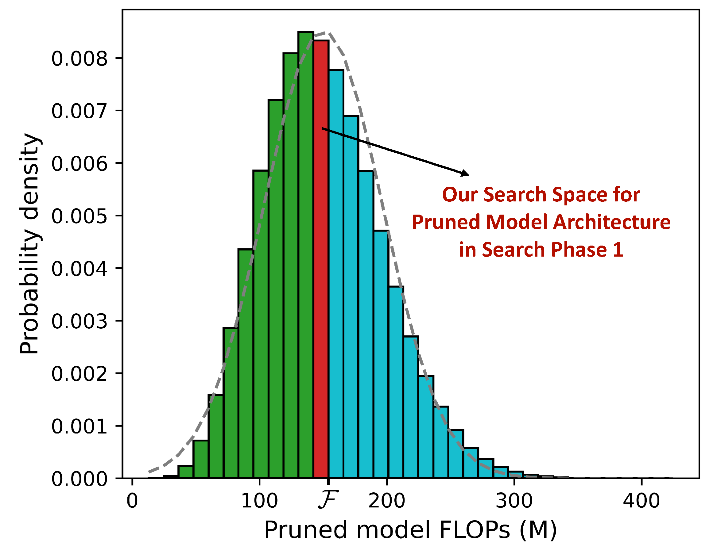
For the search space of pruned model architectures, in the context of automatic filter pruning, we often search in the space in which all models have FLOPs less than the given target , as the constraints in Equation (1). However, some models in such a search space are redundant. For example, if we have constraint M, then those models with FLOPs less than 50 M do not need to be explored, because they have little chance to be more accurate than those models with 149 M FLOPs due to the big gap between their capacity. Therefore, we further strengthen the constraints as in Equation (2). Quantitatively, we set in Equation (2) and aim to compress MobileNet [39] to have less than 150 M FLOPs ( M). We randomly sample one million pruned models to estimate the pruned model’s FLOPs distribution. The results are shown in Figure 3. As we can see, with and M, there are 540,611 pruned models (about of the total) in the search space when using Equation (1). In contrast, there are only 24,879 pruned models (about of the total) in the search space when using Equation (2), which compresses the space by about 21 times and makes the search process more efficient.
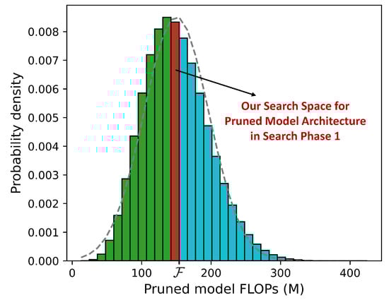
Figure 3.
Pruned model’s FLOPs distribution for MobileNet with different pruning ratios. The blue bars represent models within the original search space, while the green bars represent the reduced search space after applying the strengthened constraints.
For the search space of pruning algorithms, we pick up several pruning algorithms from previous works to form the search space, which includes pruning [14], FPGM [20], APoZ [38], and HRank [22]. These methods define the importance criterion of filters in convolution layers from different aspects. For the j-th filter in the i-th layer with weight and input X, pruning [14] defines its importance as , which is the norm of the filter; FPGM [20] defines the importance as , which is the geometric median of the filter; APoZ [38] defines the importance as , which is the non-zero ratio of the output activations; HRank [22] defines the importance as , which is the rank of the output feature maps. Among these methods, pruning and FPGM determine the importance of filters only depending on their weights; thus, both of them are data-independent. However, APoZ and HRank determine the importance of filters depending on their output feature maps, which need a set of calibration data. Different pruning algorithms define filter importance from different perspectives, and which algorithm is better depends on the specific situation (e.g., input data distribution, pre-trained weights distribution, and neural network architecture); thus, searching for the pruning algorithm for each specific layer is more appropriate. Pruning algorithms in the search space are summarized in Table 1. We further visualize the importance of filters in different convolution layers determined by different pruning algorithms, as illustrated in Figure 4.
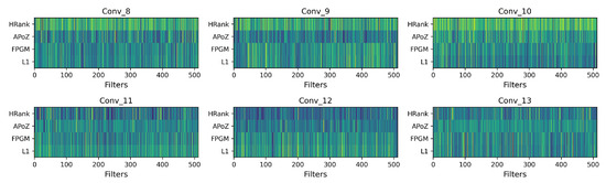
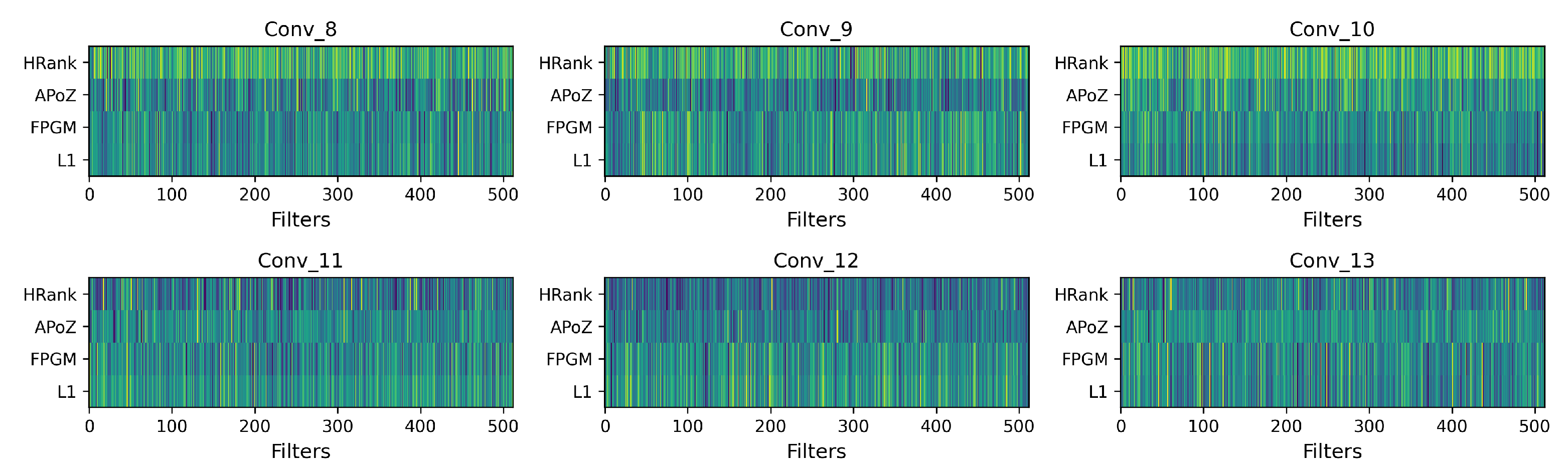
Figure 4.
Filters importance with different pruning algorithms, each subfigure demonstrates the importance of 512 filters of a convolution layer in VGG-16 [1], the x-axis represents the indices of filters and the y-axis is the different pruning algorithm. For data-dependent APoZ [38] and HRank [22], we randomly sample 1024 images from the CIFAR-10 training dataset as the calibration data to generate feature maps and calculate the filter importance. The intensity of the color indicates the importance level of the filters, with darker colors signifying greater importance.
3.3. Fast Hybrid Search
We propose a fast hybrid search method to search for the pruned model architecture and pruning algorithms simultaneously. Specifically, we separate the search process into two phases. We firstly search in a large space with an efficient but relatively inaccurate model evaluation method; then, we search in a small candidates set based on the previous results with a relatively slow but accurate model evaluation method. With such a two-phase search, we can trade-off well between accuracy and efficiency. The overall workflow is demonstrated in Figure 2.
In the first phase, we search in the search space described in Section 3.2 with the evolution algorithm. To accelerate the model evaluation, we use adaptive-BN [37] to evaluate the sampled candidate. Specifically, batch normalization is calculated as Equation (3), where x represents the input to the normalization layer, is the mean of the input, denotes the variance of the input, is a small constant added for numerical stability, and and are parameters to be learned during training that scale and shift the normalized input, respectively. The output y is the normalized and scaled input.
After the pre-trained model is pruned by the sampled candidate c and s, we firstly reset and in all batch normalization(BN) layers. Then, we use some batches of data to re-calibrate the BN layer by forward propagation, which is implemented by calculating and of each batch and updating and with momentum as in Equation (4), where and represent the mean and variance of the input for the current batch , respectively. and are the global mean and variance used in the BN layer, which are updated during training. The parameter (0 ≤ m ≤ 1) is the momentum term that controls the extent of the update, balancing between the current batch’s statistics and the existing global statistics. This updating mechanism ensures that the BN layer adapts to the data distribution in an ongoing manner throughout the training process.
Finally, we evaluate the pruned model accuracy on the validation dataset. Adaptive-BN is an efficient method for pruned model evaluation because it only needs few forward propagation to re-calibrate and .
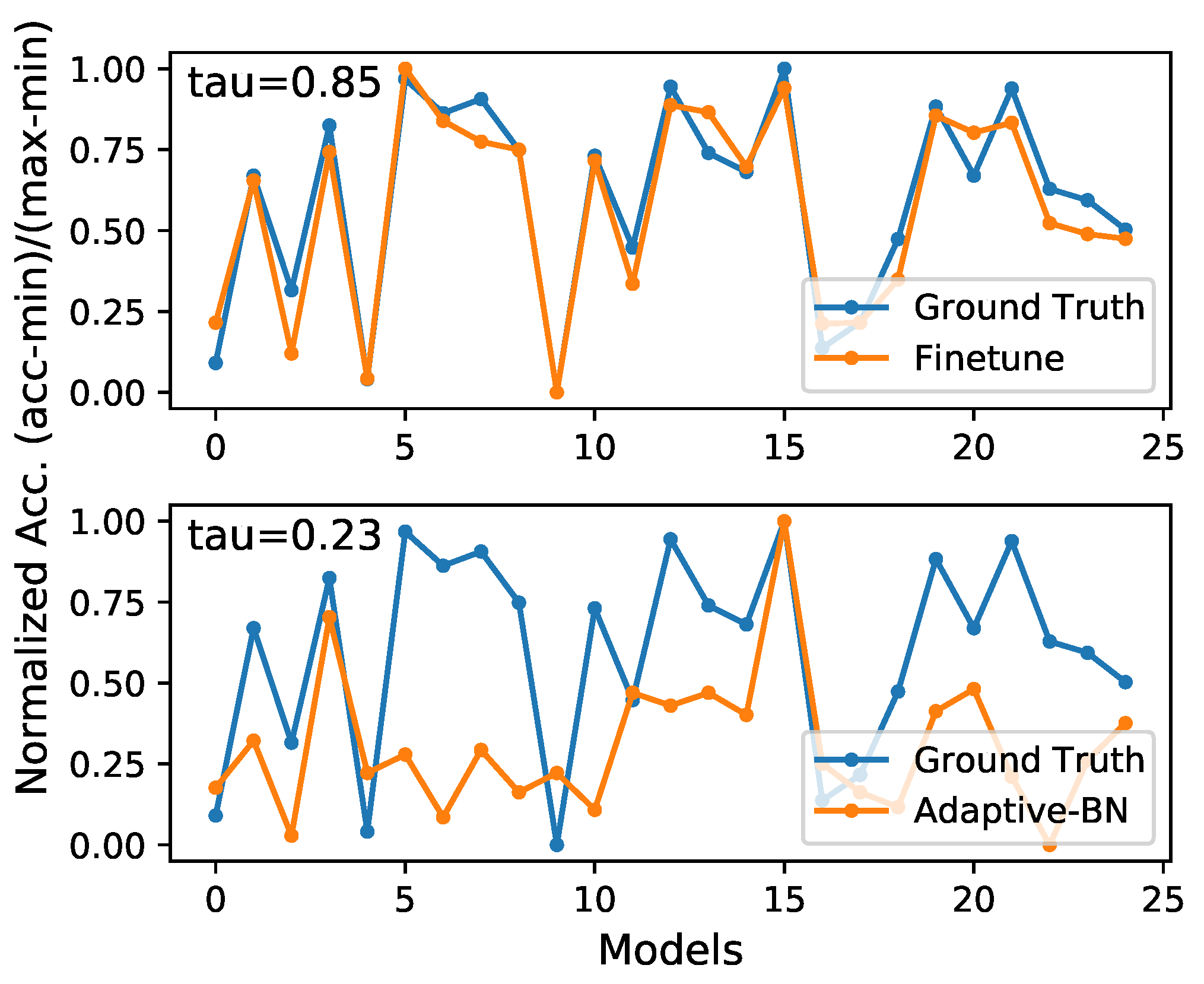
However, there is no free lunch. Adaptive-BN is efficient but not accurate enough. As illustrated in Figure 5, validation accuracy distribution evaluated by Adaptive-BN has some deviation from the ground truth. Thus, we maintain a set to store the top-K candidates in the first search phase, and we employ a more accurate model evaluation method in the second search phase.

Figure 5.
Comparison of different model evaluation methods, evaluating the pruned model by fine-tuning is more consistent with the ground truth. Experiments are pruning VGGNet with M.
In the second phase, we simply traverse all the candidates in the set , and all the candidates are evaluated by fine-tuning for few epochs. As shown in Figure 5, fine-tuning the pruned models is more accurate than adaptive-BN for the pruned model accuracy prediction.
Quantitatively, we use Kendall’s [48] to indicate the rank consistency of these two model evaluation methods with the ground truth. As demonstrated in Table 2, evaluating models by fine-tuning has a more consistent rank with the ground truth, which is , which means that is the correct rate in the result of the pairwise comparison.
Table 2.
Comparison between model evaluation methods.
In terms of time consumption, when pruning MobileNet [39] on ImageNet, fine-tuning for three epochs takes about h (with 2 V100), and adaptive-BN only takes about h, which is much faster.
Our two-phase method firstly evaluates models by adaptive-BN when searching in a huge space; then, it evaluate models by fine-tuning when searching in a small candidates set. Thus, our proposed method can trade-off well between efficiency and accuracy. The complete algorithm is shown as follows, in Algorithm 1. The fast hybrid search algorithm consists of two stages, rapid coarse screening and precise evaluation. During the rapid coarse screening phase, a search is conducted within the space of pruning ratios and the space of importance evaluation metrics using an evolutionary algorithm, resulting in a Top-K set of candidate structures. In the precise evaluation phase, the optimal compact structure is obtained by directly fine-tuning the model.
| Algorithm 1 Fast Hybrid Search Algorithm |
| Require: Model , Weights , Validation dataset , FLOPs constraint Ensure: Optimal pruning ratio and pruning algorithm Initialize candidate set Initialize pruning ratio Initialize pruning algorithm // Phase 1: Large Space Search with Adaptive-BN for each candidate in search space sampled by evolutionary algorithm do Evaluate candidate using Adaptive-BN if candidate is in top-K then Add candidate to end if end for // Phase 2: Small Space Search with Finetuning for each candidate in do Finetune the model Evaluate performance on if performance is better than current best then Update new pruning ratio Update new pruning algorithm end if end for return |
4. Experiments
The proposed hybrid search is efficient due to the two-phase search. To validate this, we conduct several experiments both on CIFAR-10 and ImageNet [41]. We prune several models, including VGGNet [1], ResNet [2], MobileNet [39], and MobileNetV2 [40], to demonstrate the effectiveness of our proposed hybrid search.
We first introduce the experiments on CIFAR-10 in Section 4.1. Specifically, we compress VGGNet on this dataset under several FLOPs constraints. Then, we conduct extensive experiments on the ImageNet in Section 4.2. Specifically, we compress several models, including ResNet series and MobileNet series. Finally, we conduct an ablation study in Section 4.3.
4.1. Experiments on CIFAR-10
We prune VGGNet [1] on CIFAR-10. During the search process, as VGGNet for CIFAR-10 has 13 convolutional layers, each candidate is encoded as a vector of to denote pruned model architecture and to denote pruning algorithms. In the first search phase, each candidate is evaluated by adaptive-BN; after that, the top 30 candidates with the highest validation accuracy are inserted into a set . Then, in the second search phase, each candidate in is evaluated by 10 epochs of fine-tuning. We set the batch size to 256 and the initial learning rate to 0.1. We first warm-up over five epochs and then anneal down to zero with a cosine strategy.
After the search process has finished, we fine-tune the pruned model with the highest validation accuracy in over 300 epochs, with all the other hyperparameters remaining the same as in the the second search phase, except the training epochs. We conduct simple data augmentation on the CIFAR-10 dataset: the images are first randomly cropped with padding, then processed with random flipping and random cutout, and finally normalized with their mean and standard deviation.
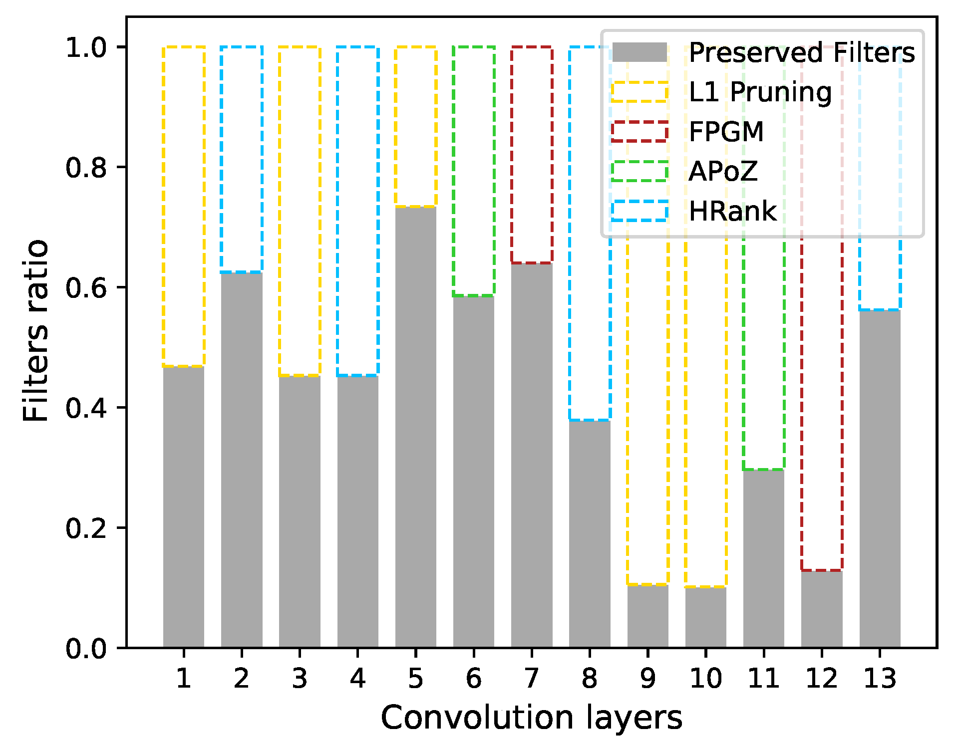
We constrain pruned models to having less than 70M/100M/150M FLOPs. Experimental results are shown in Table 3. We beat several other methods with the same or fewer FLOPs, including pruning [14], SSS [49], HRank [22], and ABCPruner [21]. The pruned VGGNet is visualized in Figure 6.
Table 3.
Top-1 accuracy of VGGNet on CIFAR-10. ’#’ denotes ’number of’.
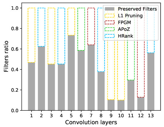
Figure 6.
Visualization of the pruned VGGNet with M.
4.2. Experiments on ImageNet
The proposed hybrid search is efficient and can be used to directly search on ImageNet [41], which consists of 1000 classes, with million training images and 50,000 validation images. We prune ResNet [2], MobileNet [39], and MobileNetV2 [40] using the proposed hybrid search and validate them on ImageNet [41].
As ImageNet [41] is much larger than CIFAR-10, we reduce the fine-tuning epochs in the the second search phase from ten to three with one warm-up epoch. All the other hyper-parameters are the same as for CIFAR-10, as seen in Section 4.1. After the search process is finished, we fine-tune the best pruned model over 120 epochs with all other hyper-parameters the same as in Section 4.1.
We also conduct simple data augmentation and pre-processing for ImageNet: images are randomly cropped and flipped, then resized to , and finally normalized with their mean and standard deviation.
4.2.1. Pruning ResNets
We prune ResNet-18, ResNet-34, and ResNet-50. Experimental results are shown in Table 4. Our proposed hybrid search shows a clear performance improvement compared to several SOTA methods, including ABCPruner [21] and MetaPruning [47]. More comparisons on ResNet-50 are demonstrated in Table 5. The experiments show that, when compressing to both 1G FLOPs (higher compression rate) and 2G FLOPs (lower compression rate), hybrid search is generally better than other methods. Notably, when we prune ResNet-50 further to have only 600M FLOPs, our method still achieves a top-1 accuracy, beating many other methods, such as SSS-26 [49] and ThiNet-50 [18], even though they have more than 1G FLOPs.
Table 4.
Pruning results of ResNet on ImageNet. ’#’ denotes ’number of’.
Table 5.
Pruning results of ResNet-50 on ImageNet.
4.2.2. Pruning MobileNets
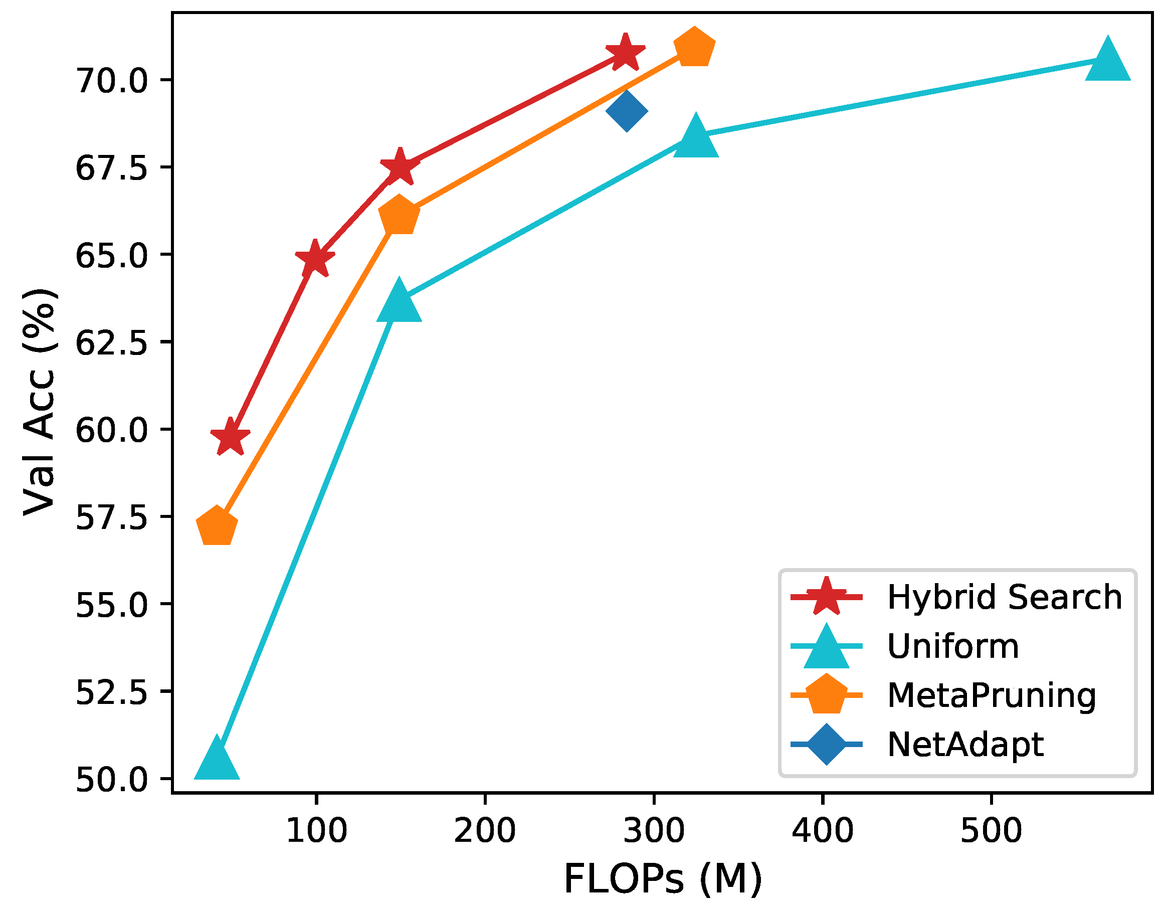
We prune MobileNet [39] and MobileNetV2 [40] on ImageNet. The results are summarized in Figure 7, Table 6, and Table 7. Our proposed hybrid search shows a clear improvement in performance compared to the other baselines, including Uniform Pruning, AMC [19], and MetaPruning [47]. Specifically, as shown in Figure 7 and Table 6, hybrid search shows the best top-1 accuracy at all 50M, 150M, and 285M FLOPs. In addition, our method tends to have a significant increase in performance when the model is compressed aggressively.
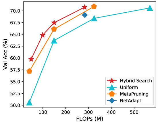
Figure 7.
Comparison of different automatic pruning methods for pruning MobileNet [39] to different FLOPs.
Table 6.
Pruning results of MobileNet on ImageNet.
Table 7.
Pruning results of MobileNetV2 on ImageNet.
Specifically, when compressing MobileNet to 150M, we have a top-1 accuracy, which is higher than MetaPruning. When compressing the network to 50M, we have a top-1 accuracy, which is higher than MetaPruning. This indicates that our proposed hybrid search has more advantages in terms of model deployment.
4.3. Ablation Study
We also conduct an ablation study to validate the effectiveness of each component in our hybrid search method. Specifically, we firstly validate the effectiveness of searching for the pruning algorithm for each convolution layer to be pruned. We fix c in the two-search phase, and only search for the pruned model architecture. When we prune VGGNet with M, the experiment results of which are summarized in Table 8, we can observe that searching for the pruned model architecture and pruning algorithms simultaneously yields a better compact model.
Table 8.
Pruning results with different pruning algorithms.
Then, we validate the effectiveness of the two-phase search. We prune MobileNet with M. When we skip the first search phase by randomly sampling 30 candidates as , and fine-tune all these candidates for a few epochs, we can only find the compact model with top-1 accuracy after fine-tuning the model to convergence. When we skip the second search phase by removing the candidates set and just fine-tune the best model evaluated by adaptive-BN in the the first search phase to convergence, we can obtain the compact model with top-1 accuracy. The experiments are summarized in Table 9.
Table 9.
Pruning results after removing one of the search phases. ”✓” indicates that the phase was included in the model, and ”✗” indicates that the phase was excluded from the model.
5. Conclusions
In this paper, we propose a novel hybrid search method for automatic filter pruning. We search for the pruned model architecture and pruning algorithms simultaneously for the first time. We innovatively undertake the task of searching for both the pruned model architecture and the pruning algorithms in tandem, marking the first instance in the literature wherein these two critical components of model optimization are optimized simultaneously. Moreover, our proposed method separates the search process into two phases; thus, we can trade-off well between the search efficiency and effectiveness. Our proposed method effectively surpasses other pruning methods, which include conventional methods and AutoML-based methods. Our proposed hybrid search method can be further applied in automatic model quantization, to search for the quantization bits and quantizer at the same time.
Author Contributions
Conceptualization, G.L., L.T. and X.Z.; methodology, G.L. and L.T.; software, G.L. and L.T.; validation, G.L. and L.T.; formal analysis, G.L.; investigation, G.L.; resources, G.L.; data curation, G.L.; writing—original draft preparation, G.L.; writing—review and editing, G.L. and L.T.; visualization, G.L.; supervision, X.Z.; project administration, X.Z.; funding acquisition, X.Z. All authors have read and agreed to the published version of the manuscript.
Funding
This work was supported by National Key R&D Program of China (No. 2022ZD0118202), the National Science Fund for Distinguished Young Scholars (No. 62025603), the National Natural Science Foundation of China (No. U21B2037, No. U22B2051, No. 62176222, No. 62176223, No. 62176226, No. 62072386, No. 62072387, No. 62072389, No. 62002305 and No. 62272401), and the Natural Science Foundation of Fujian Province of China (No. 2021J01002, No. 2022J06001).
Data Availability Statement
Data are contained within the article.
Conflicts of Interest
The authors declare no conflicts of interest.
References
- Simonyan, K.; Zisserman, A. Very deep convolutional networks for large-scale image recognition. arXiv 2014, arXiv:1409.1556. [Google Scholar]
- He, K.; Zhang, X.; Ren, S.; Sun, J. Deep residual learning for image recognition. In Proceedings of the IEEE Conference on Computer Vision and Pattern Recognition, Las Vegas, NV, USA, 27–30 June 2016; pp. 770–778. [Google Scholar]
- Hu, J.; Shen, L.; Sun, G. Squeeze-and-excitation networks. In Proceedings of the IEEE Conference on Computer Vision and Pattern Recognition, Salt Lake City, UT, USA, 18–23 June 2018; pp. 7132–7141. [Google Scholar]
- Redmon, J.; Divvala, S.; Girshick, R.; Farhadi, A. You only look once: Unified, real-time object detection. In Proceedings of the IEEE Conference on Computer Vision and Pattern Recognition, Las Vegas, NV, USA, 27–30 June 2016; pp. 779–788. [Google Scholar]
- Liu, W.; Anguelov, D.; Erhan, D.; Szegedy, C.; Reed, S.; Fu, C.Y.; Berg, A.C. Ssd: Single shot multibox detector. In Proceedings of the European Conference on Computer Vision, Amsterdam, The Netherlands, 11–14 October 2016; Springer: Cham, Switzerland, 2016; pp. 21–37. [Google Scholar]
- Chen, L.C.; Papandreou, G.; Kokkinos, I.; Murphy, K.; Yuille, A.L. Deeplab: Semantic image segmentation with deep convolutional nets, atrous convolution, and fully connected crfs. IEEE Trans. Pattern Anal. Mach. Intell. 2017, 40, 834–848. [Google Scholar] [CrossRef] [PubMed]
- Ronneberger, O.; Fischer, P.; Brox, T. U-net: Convolutional networks for biomedical image segmentation. In Proceedings of the International Conference on Medical Image Computing and Computer-Assisted Intervention, Munich, Germany, 5–9 October 2015; Springer: Cham, Switzerland, 2015; pp. 234–241. [Google Scholar]
- Zhang, S.; Xia, X.; Wang, Z.; Chen, L.H.; Liu, J.; Wu, Q.; Liu, T. IDEAL: Influence-Driven Selective Annotations Empower In-Context Learners in Large Language Models. arXiv 2023, arXiv:2310.10873. [Google Scholar]
- Pan, W.; Gao, T.; Zhang, Y.; Zheng, X.; Shen, Y.; Li, K.; Hu, R.; Liu, Y.; Dai, P. Semi-Supervised Blind Image Quality Assessment through Knowledge Distillation and Incremental Learning. In Proceedings of the Thirty-Eighth AAAI Conference on Artificial Intelligence, Vancouver, BC, Canada, 20–27 February 2024. [Google Scholar]
- Zhang, Y.; Ji, R.; Fan, X.; Wang, Y.; Guo, F.; Gao, Y.; Zhao, D. Search-based depth estimation via coupled dictionary learning with large-margin structure inference. In Proceedings of the European Conference on Computer Vision, Amsterdam, The Netherlands, 11–14 October 2016; Springer: Cham, Switzerland; pp. 858–874. [Google Scholar]
- Zhang, Y.; Fan, X.; Zhao, D. Semisupervised learning-based depth estimation with semantic inference guidance. Sci. China Technol. Sci. 2022, 65, 1098–1106. [Google Scholar] [CrossRef]
- Zhang, Y.; Jiang, F.; Rho, S.; Liu, S.; Zhao, D.; Ji, R. 3D object retrieval with multi-feature collaboration and bipartite graph matching. Neurocomputing 2016, 195, 40–49. [Google Scholar] [CrossRef]
- Qin, G.; Hu, R.; Liu, Y.; Zheng, X.; Liu, H.; Li, X.; Zhang, Y. Data-Efficient Image Quality Assessment with Attention-Panel Decoder. arXiv 2023, arXiv:2304.04952. [Google Scholar] [CrossRef]
- Li, H.; Kadav, A.; Durdanovic, I.; Samet, H.; Graf, H.P. Pruning filters for efficient convnets. arXiv 2016, arXiv:1608.08710. [Google Scholar]
- Han, S.; Mao, H.; Dally, W.J. Deep compression: Compressing deep neural networks with pruning, trained quantization and huffman coding. arXiv 2015, arXiv:1510.00149. [Google Scholar]
- Liu, Z.; Sun, M.; Zhou, T.; Huang, G.; Darrell, T. Rethinking the value of network pruning. arXiv 2018, arXiv:1810.05270. [Google Scholar]
- Liu, Z.; Li, J.; Shen, Z.; Huang, G.; Yan, S.; Zhang, C. Learning efficient convolutional networks through network slimming. In Proceedings of the IEEE International Conference on Computer Vision, Venice, Italy, 22–29 October 2017; pp. 2736–2744. [Google Scholar]
- Luo, J.H.; Wu, J.; Lin, W. Thinet: A filter level pruning method for deep neural network compression. In Proceedings of the IEEE International Conference on Computer Vision, Venice, Italy, 22–29 October 2017; pp. 5058–5066. [Google Scholar]
- He, Y.; Lin, J.; Liu, Z.; Wang, H.; Li, L.J.; Han, S. Amc: Automl for model compression and acceleration on mobile devices. In Proceedings of the European Conference on Computer Vision (ECCV), Munich, Germany, 8–14 September 2018; pp. 784–800. [Google Scholar]
- He, Y.; Liu, P.; Wang, Z.; Hu, Z.; Yang, Y. Filter pruning via geometric median for deep convolutional neural networks acceleration. In Proceedings of the IEEE Conference on Computer Vision and Pattern Recognition, Long Beach, CA, USA, 5–20 June 2019; pp. 4340–4349. [Google Scholar]
- Lin, M.; Ji, R.; Zhang, Y.; Zhang, B.; Wu, Y.; Tian, Y. Channel Pruning via Automatic Structure Search. In Proceedings of the International Joint Conference on Artificial Intelligence (IJCAI), Yokohama, Japan, 7–15 January 2021; pp. 673–679. [Google Scholar]
- Lin, M.; Ji, R.; Wang, Y.; Zhang, Y.; Zhang, B.; Tian, Y.; Shao, L. Hrank: Filter Pruning using High-Rank Feature Map. In Proceedings of the IEEE/CVF Conference on Computer Vision and Pattern Recognition, Seattle, WA, USA, 13–19 June 2020; pp. 1529–1538. [Google Scholar]
- Courbariaux, M.; Bengio, Y.; David, J.P. Binaryconnect: Training deep neural networks with binary weights during propagations. In Proceedings of the 28th International Conference on Neural Information Processing Systems, Cambridge, MA, USA, 7–12 December 2015; pp. 3123–3131. [Google Scholar]
- Ge, T.; He, K.; Ke, Q.; Sun, J. Optimized product quantization for approximate nearest neighbor search. In Proceedings of the IEEE Conference on Computer Vision and Pattern Recognition, Portland, OR, USA, 23–28 June 2013; pp. 2946–2953. [Google Scholar]
- Zhou, S.; Wu, Y.; Ni, Z.; Zhou, X.; Wen, H.; Zou, Y. Dorefa-net: Training low bitwidth convolutional neural networks with low bitwidth gradients. arXiv 2016, arXiv:1606.06160. [Google Scholar]
- Lin, M.; Ji, R.; Xu, Z.; Zhang, B.; Wang, Y.; Wu, Y.; Huang, F.; Lin, C.W. Rotated Binary Neural Network. In Proceedings of the 34th International Conference on Neural Information Processing Systems, Vancouver BC, Canada, 6–12 December 2020. [Google Scholar]
- Hinton, G.; Vinyals, O.; Dean, J. Distilling the knowledge in a neural network. arXiv 2015, arXiv:1503.02531. [Google Scholar]
- Phuong, M.; Lampert, C.H. Distillation-based training for multi-exit architectures. In Proceedings of the IEEE International Conference on Computer Vision, Seoul, Republic of Korea, 27 October–2 November 2019; pp. 1355–1364. [Google Scholar]
- Yang, C.; Xie, L.; Qiao, S.; Yuille, A.L. Training deep neural networks in generations: A more tolerant teacher educates better students. In Proceedings of the AAAI Conference on Artificial Intelligence, Honolulu, HI, USA, 27 January–1 February 2019; Volume 33, pp. 5628–5635. [Google Scholar]
- Xie, Q.; Luong, M.T.; Hovy, E.; Le, Q.V. Self-training with noisy student improves imagenet classification. In Proceedings of the IEEE/CVF Conference on Computer Vision and Pattern Recognition, Seattle, WA, USA, 13–19 June 2020; pp. 10687–10698. [Google Scholar]
- Cho, J.H.; Hariharan, B. On the efficacy of knowledge distillation. In Proceedings of the IEEE International Conference on Computer Vision, Seoul, Republic of Korea, 27 October–2 November 2019; pp. 4794–4802. [Google Scholar]
- Zhang, S.; Jia, F.; Wang, C.; Wu, Q. Targeted hyperparameter optimization with lexicographic preferences over multiple objectives. In Proceedings of the Eleventh International Conference on Learning Representations, Kigali, Rwanda, 1– 5 May 2023. [Google Scholar]
- Zhang, S.; Wu, Y.; Zheng, Z.; Wu, Q.; Wang, C. HyperTime: Hyperparameter Optimization for Combating Temporal Distribution Shifts. arXiv 2023, arXiv:2305.18421. [Google Scholar]
- He, Y.; Zhang, X.; Sun, J. Channel pruning for accelerating very deep neural networks. In Proceedings of the IEEE International Conference on Computer Vision, Venice, Italy, 22–29 October 2017; pp. 1389–1397. [Google Scholar]
- Zheng, X.; Yang, C.; Zhang, S.; Wang, Y.; Zhang, B.; Wu, Y.; Wu, Y.; Shao, L.; Ji, R. Ddpnas: Efficient neural architecture search via dynamic distribution pruning. Int. J. Comput. Vis. 2023, 131, 1234–1249. [Google Scholar] [CrossRef]
- Zhang, S.; Zheng, X.; Yang, C.; Li, Y.; Wang, Y.; Chao, F.; Wang, M.; Li, S.; Yang, J.; Ji, R. You only compress once: Towards effective and elastic bert compression via exploit-explore stochastic nature gradient. arXiv 2021, arXiv:2106.02435. [Google Scholar]
- Li, B.; Wu, B.; Su, J.; Wang, G.; Lin, L. Eagleeye: Fast sub-net evaluation for efficient neural network pruning. arXiv 2020, arXiv:2007.02491. [Google Scholar]
- Hu, H.; Peng, R.; Tai, Y.W.; Tang, C.K. Network trimming: A data-driven neuron pruning approach towards efficient deep architectures. arXiv 2016, arXiv:1607.03250. [Google Scholar]
- Howard, A.G.; Zhu, M.; Chen, B.; Kalenichenko, D.; Wang, W.; Weyand, T.; Andreetto, M.; Adam, H. Mobilenets: Efficient convolutional neural networks for mobile vision applications. arXiv 2017, arXiv:1704.04861. [Google Scholar]
- Sandler, M.; Howard, A.; Zhu, M.; Zhmoginov, A.; Chen, L.C. Mobilenetv2: Inverted residuals and linear bottlenecks. In Proceedings of the IEEE Conference on Computer Vision and Pattern Recognition, Salt Lake City, UT, USA, 18–23 June 2018; pp. 4510–4520. [Google Scholar]
- Deng, J.; Dong, W.; Socher, R.; Li, L.J.; Li, K.; Fei-Fei, L. Imagenet: A large-scale hierarchical image database. In Proceedings of the 2009 IEEE Conference on Computer Vision and Pattern Recognition, Miami, FL, USA, 20–25 June 2009; IEEE: Piscataway, NJ, USA, 2009; pp. 248–255. [Google Scholar]
- Frankle, J.; Carbin, M. The lottery ticket hypothesis: Finding sparse, trainable neural networks. arXiv 2018, arXiv:1803.03635. [Google Scholar]
- Denton, E.L.; Zaremba, W.; Bruna, J.; LeCun, Y.; Fergus, R. Exploiting linear structure within convolutional networks for efficient evaluation. In Proceedings of the 27th International Conference on Neural Information Processing Systems, Montreal, QC, Canada, 8–13 December 2014; pp. 1269–1277. [Google Scholar]
- Lebedev, V.; Ganin, Y.; Rakhuba, M.; Oseledets, I.; Lempitsky, V. Speeding-up convolutional neural networks using fine-tuned cp-decomposition. arXiv 2014, arXiv:1412.6553. [Google Scholar]
- He, Y.; Kang, G.; Dong, X.; Fu, Y.; Yang, Y. Soft filter pruning for accelerating deep convolutional neural networks. arXiv 2018, arXiv:1808.06866. [Google Scholar]
- Ioffe, S.; Szegedy, C. Batch normalization: Accelerating deep network training by reducing internal covariate shift. arXiv 2015, arXiv:1502.03167. [Google Scholar]
- Liu, Z.; Mu, H.; Zhang, X.; Guo, Z.; Yang, X.; Cheng, K.T.; Sun, J. Metapruning: Meta learning for automatic neural network channel pruning. In Proceedings of the IEEE International Conference on Computer Vision, Seoul, Republic of Korea, 27 October–2 November 2019; pp. 3296–3305. [Google Scholar]
- Kendall, M.G. A new measure of rank correlation. Biometrika 1938, 30, 81–93. [Google Scholar] [CrossRef]
- Huang, Z.; Wang, N. Data-driven sparse structure selection for deep neural networks. In Proceedings of the European Conference on Computer Vision (ECCV), Munich, Germany, 8–14 September 2018; pp. 304–320. [Google Scholar]
- Lin, S.; Ji, R.; Yan, C.; Zhang, B.; Cao, L.; Ye, Q.; Huang, F.; Doermann, D. Towards optimal structured cnn pruning via generative adversarial learning. In Proceedings of the IEEE Conference on Computer Vision and Pattern Recognition, Long Beach, CA, USA, 15–20 June 2019; pp. 2790–2799. [Google Scholar]
- Ning, X.; Zhao, T.; Li, W.; Lei, P.; Wang, Y.; Yang, H. DSA: More Efficient Budgeted Pruning via Differentiable Sparsity Allocation. arXiv 2020, arXiv:2004.02164. [Google Scholar]
- Dong, X.; Huang, J.; Yang, Y.; Yan, S. More is less: A more complicated network with less inference complexity. In Proceedings of the IEEE Conference on Computer Vision and Pattern Recognition, Honolulu, HI, USA, 21–26 July 2017; pp. 5840–5848. [Google Scholar]
- Yu, J.; Huang, T. AutoSlim: Towards One-Shot Architecture Search for Channel Numbers. arXiv 2019, arXiv:1903.11728. [Google Scholar]
- Yang, T.J.; Howard, A.; Chen, B.; Zhang, X.; Go, A.; Sandler, M.; Sze, V.; Adam, H. Netadapt: Platform-aware neural network adaptation for mobile applications. In Proceedings of the European Conference on Computer Vision (ECCV), Munich, Germany, 8–14 September 2018; pp. 285–300. [Google Scholar]
Disclaimer/Publisher’s Note: The statements, opinions and data contained in all publications are solely those of the individual author(s) and contributor(s) and not of MDPI and/or the editor(s). MDPI and/or the editor(s) disclaim responsibility for any injury to people or property resulting from any ideas, methods, instructions or products referred to in the content. |
© 2024 by the authors. Licensee MDPI, Basel, Switzerland. This article is an open access article distributed under the terms and conditions of the Creative Commons Attribution (CC BY) license (https://creativecommons.org/licenses/by/4.0/).