Abstract
The thermal vacuum test (TVT) is an important verification process in the development of spacecraft and load. There are often multiple temperature points on the device under test (DUT) that require control. The interaction among multiple channels poses a challenge for temperature control in the TVT. To solve this problem, a multi-channel Smith proportional–integral–derivative (PID) controller based on a grouping neural network (Grouping-NN) is proposed. Firstly, the mathematical derivation for a typical multi-channel temperature control model of the TVT is carried out. Then, the multi-channel interaction system is identified using a Grouping-NN to predict the output temperature of each channel by grouping the hidden layer neurons according to the number of channels. Finally, two Grouping-NNs are utilized to update the Smith predictor, and the time-delay error is fed back to the PID controller, which is used to optimize the control effect of the multi-channel interaction system under high time delay. The proposal is compared with the traditional PID controller and Smith predictor-based PID controller through simulation. The simulation results show that the proposed method has better suppression of overshooting. In addition, the algorithm is verified by controlling the temperature of six channels in a practical thermal vacuum test.
1. Introduction
The thermal vacuum test, which provides an environment close to a vacuum and simulates high temperature caused by solar irradiation as well as low temperature without the sun [1], is an important procedure in the development of spacecraft and loads to test their ultimate working performance [2,3,4]. The thermal vacuum chamber (TVC) is the most important equipment of the TVT, and can provide an environment close to vacuum by extracting air. During the TVT, the DUT, temperature sensors, and infrared heating equipment are all placed in the chamber. By adjusting the output power of the heating equipment in real time, the temperature of the measuring point on the DUT is stabilized to the set value [5,6,7]. The nonlinear model predictive controller (NMPC) is established in the TVT to control the shroud temperature and change the DUT temperature to the set value [8]. In order to test the performance of the DUT at extreme temperature, the temperature control requirements inside the chamber are strict, and the PID controller is generally used in the TVT to achieve precise temperature control. In [9], a TVT based on silicone oil cooling was constructed, and the design of an automatic temperature control based on fuzzy PID control was carried out, and the Cohen–Coon method was used to adjust the initial PID. In [10], an adaptive PID controller based on a radial basis function (RBF) neural network was designed for a thermal vacuum test. The control strategy can automatically adjust the neural network weights and the control parameters of the PID controller online to reduce the system tracking overshoot.
The proportional, integral, and differential coefficients of PID controllers need to be tuned before control [11]. For some scenarios where the coefficients need to be adjusted in real time, some adaptive control methods have been proposed, such as fuzzy PID methods [12,13,14] and neural network-based PID methods [10,15]. In addition, in order to reduce the impact of time delay, many Smith predictor-based methods are used to modify PID controllers [16,17]. Due to the nonlinear heating response of infrared radiation heaters, as well as the inconsistent heating transfer function at high and low temperatures [18], it is extremely important to identify the transfer function of the system. The major system identification methods include the step response method, least squares method, neural network method, etc. In [19], Xu derived a Newtonian iterative algorithm that can be used to identify the parameters of second-order systems from experimental data on step response. In [20], the study uses three-layer feed-forward neural networks to estimate the transfer function model, deriving the mathematical relationship between the ARMA and ANN models.
These methods have been validated to have good accuracy on a single input/single output (SISO) control system. However, in the TVT, larger DUTs are often tested, requiring more heaters to control multiple temperature nodes on the DUT. For this multi-input/multi-output (MIMO) control system, there is interaction among channels. Especially in multi-channel temperature control applications, the channel that reaches the set temperature earliest will continue to be heated up under the action of adjacent heaters, leading to a large overshoot. In the TVT, if the local temperature of the DUT exceeded its limit temperature significantly or for a long time, it may have irreversible effects on the performance of the device.
Due to the complexity of MIMO control applications, different studies have proposed various optimization strategies for respective systems. Hagiwara et al. modeled the input–output characteristics as well as the disturbance attenuation characteristics for the MIMO system, and optimized the PID controller to attenuate the unknown disturbances [21,22]. Falguni proposed an LQR-based PID controller for a 2-DOF MIMO system. The method addresses the interaction of two cross-coupled channels by introducing state feedback of the augmented uncertain system in the PID controller [23]. Ignacio presents a model-free goal-based algorithm for MIMO PID self-tuning. The control disorder caused by frequent regulation of multiple control channels is avoided by the deep reinforcement learning-based adaptive structure. [24]. In [25], the article analyzes the model-free PID tuning methods for the MIMO system and uses the simultaneous perturbation stochastic approximation (SPSA) method in MIMO plants. The performance of several SPSA-based PID tuning methods for MIMO systems is compared, and the effect of disturbances on MIMO PID controllers is analyzed. Stephen et al. view MIMO PID controllers as an optimization problem of non-convex quadratic matrix inequalities. By replacing non-convex matrix inequalities with linear matrix inequality constraints, the calculation and iteration process are simplified, achieving the coefficients tuning of MIMO PID controllers [26]. Wang proposed a parameter identification method for MIMO systems, using an auxiliary method and a data filter to identify the MIMO system with ARMA noise as interference [27].
In most of the MIMO controller applications, the interaction among channels remains a problem that needs to be continuously optimized. For the multi-channel TVT, channel interactions and time delay are the key points to be considered. We introduce a neural network system identifier to predict the temperatures of the interacting channels. The MIMO system identifier is applied to the controller with a Smith predictor, and a Grouping-NN-based Smith PID controller is proposed. The main contributions of this paper are as follows:
- (1)
- Based on the first-order plus dead-time (FOPDT) transfer function model, a discrete multi-channel mathematical model of the interaction system is established.
- (2)
- A grouping neural network (Grouping-NN) is proposed to be used for system identification of the multi-channel interaction environment.
- (3)
- Combine two Grouping-NNs for updating the time-delay model and the model without time delay of the Smith predictor to optimize the PID controller.
The remainder of the paper is organized as follows. Section 2 introduces the control system components of the TVT and derives a mathematical model of the multi-channel interactions under this system. Section 3 describes the proposed Grouping-NN method and its combination with the Smith PID controller. System identification simulation and temperature control simulation of multi-channel interactions are presented and discussed in Section 4. Section 5 describes a practical multi-channel interaction experiment and analyzes the controller’s performance. Finally, conclusions are given in Section 6.
2. Preliminary
This section introduces the components of a temperature control system in the TVT, and models the transfer function of a multi-channel heating system.
2.1. The Structure of Temperature Control System
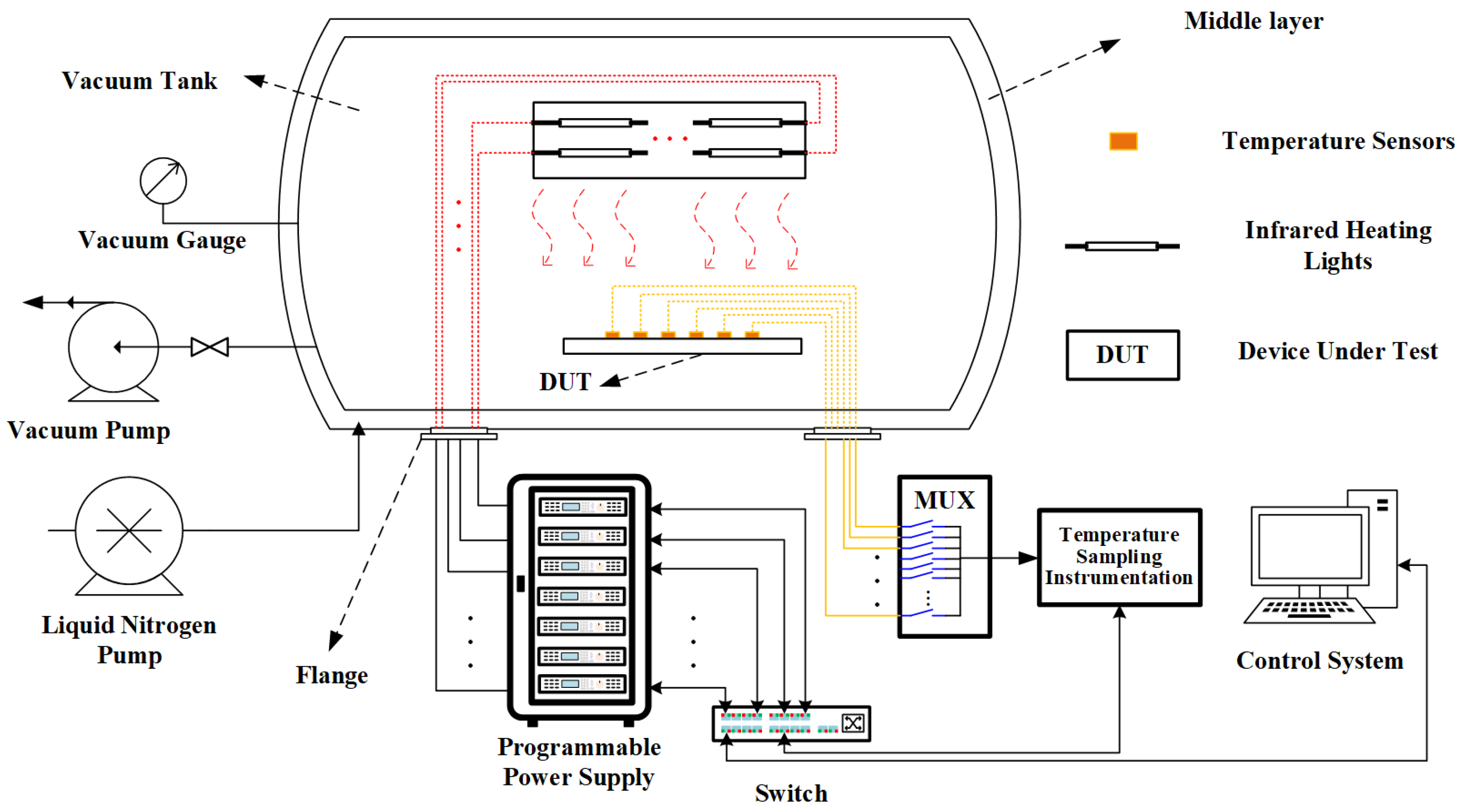
The TVT verifies the DUT at high and low temperatures in a near-vacuum environment. The tests are conducted using a multi-layer TVC to provide a low-pressure environment and a low-temperature background. A vacuum pump is used to extract air from the chamber, and a cold plate is utilized to assist in further reducing the pressure. The middle layer is between the inner and outer walls of the vacuum chamber, which is lined with spiral pipes that can fill with liquid nitrogen to provide heat sinking for the chamber.
The temperature control system for the TVT consists of temperature sensors, sampling equipment, heaters, programmable power supplies, and a host computer, and is shown in Figure 1. The temperature sensors, heaters, and DUT are arranged in the TVC according to the test requirements. Depending on the temperature range of the TVT, the temperature sensor is generally selected as a T-type thermocouple, which is attached to the surface of the DUT. These sensors are connected via a flange to temperature-sampling equipment outside the TVC, which sends the temperature data to the host computer through the Ethernet. According to the temperature data, the host computer calculates the output current of heaters by running the control program. Meanwhile, the calculated current values are sent to programmable power supplies to implement the temperature control.
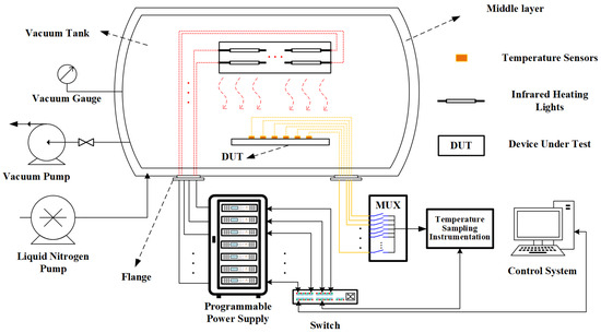
Figure 1.
The structure of the infrared radiation temperature control system in the TVT. The vacuum chamber shown is a cross−sectional view.
The heater needs to be chosen from the infrared heating cage, infrared heating tube, etc., according to the type of DUT. Since infrared heating tubes are more sensitive and difficult to control, this experiment uses infrared heating tubes as an example to verify the proposed algorithm. When multiple infrared heating tubes are operating at the same time, the heat radiated from each heater affects the adjacent temperature control area, which is called multi-channel interaction. This makes the temperature adjustment of each control area complicated.
2.2. The Transfer Function of Multi-Channel Heating System
The infrared radiation temperature control system utilizes infrared radiation to heat objects in space. Due to different absorption efficiencies from DUTs, infrared radiation often exhibits nonlinear and time-delay characteristics in temperature control. The transfer function of an infrared radiation temperature control system is a high-order model, which brings a challenge to the design of temperature control systems. Therefore, in the TVT, the model of the infrared radiation temperature control system is approximated to a FOPDT model, whose transfer function is shown in Equation (1).
where K is the magnification factor, T denotes the time constant, and indicates the time delay.
For a multi-channel interaction system, assuming that the same specification heater is used for each channel, the transfer function can be approximated as Equation (2).
where is the influence coefficient of the different heaters on the current temperature sensor.
Equation (3) utilizes the bilinear transformation method to discretize the transfer function. The is the sample period.
In practice, the transfer function in the algorithm is mostly in the form of a differential equation, which is easy to implement. The differential equation for the transfer function of the multi-channel interaction system is shown in Equations (4)–(6).
where N indicates the number of channels. In the thermal vacuum test, a channel is defined as a heater with a sensor directly opposite to it. and are the system input and output, respectively, denotes the input value of the i-th channel at moment k, and indicates the output value of the current channel. In a multi-channel interaction transfer function, the input is the current value of the heating device and the output is the temperature.
3. Proposed Method
In this section, a temperature control system is designed for a high time-delay characteristic and multi-channel interaction environment. This control system incorporates a conventional PID controller and a grouping neural network (Grouping-NN)-based multi-channel identifier. The Grouping-NN is used to predict the temperature in the presence of the interaction with multiple heating channels.
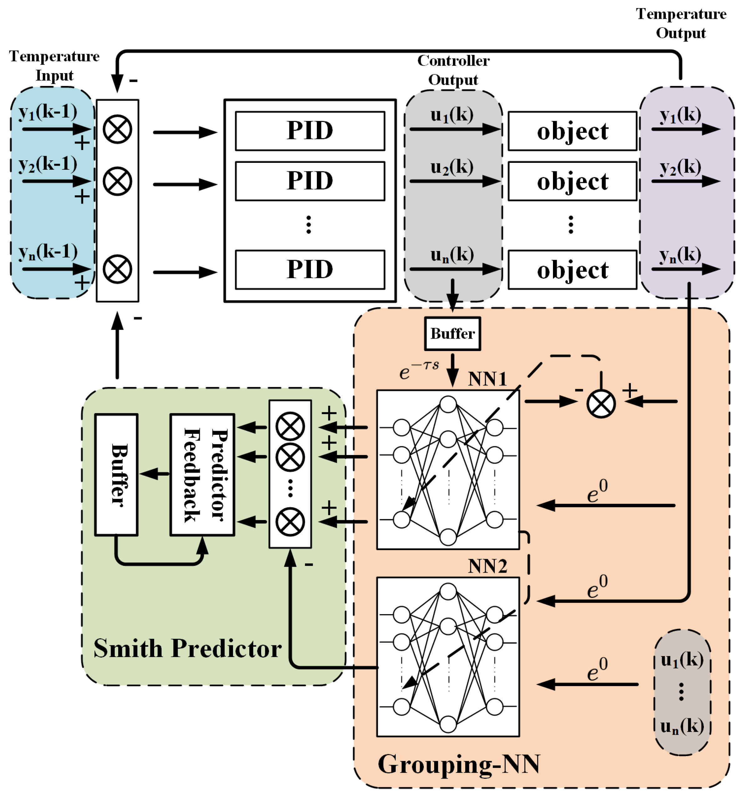
Based on the principle of the Smith predictor, two neural networks are used to predict the time-delay error. The block diagram of the proposed control system is shown in Figure 2. Each part of the system is described as follows.
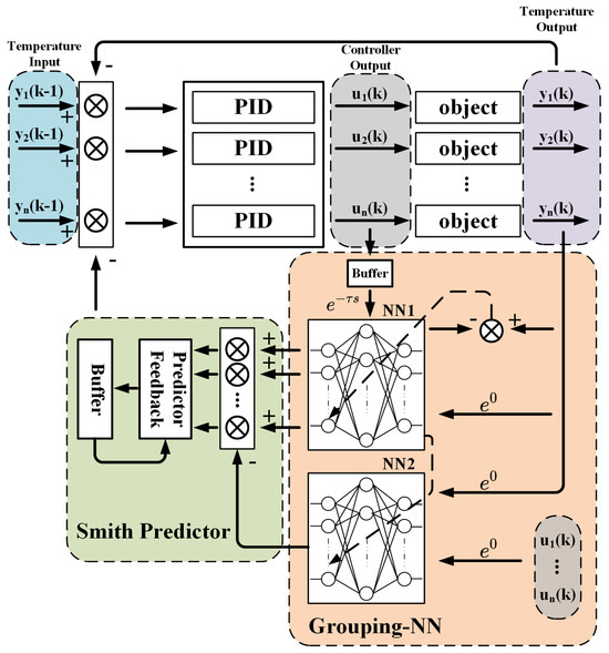
Figure 2.
Block diagram of the multi−channel Grouping−NN Smith PID controller. Multiple PIDs, Grouping−NNs, and the Smith predictor are the main parts of this controller.
3.1. PID Controller
The PID controller is the basic and the most common module in a discrete control system. The input of the PID controller is the deviation between the set value and the measured value. Proportional operation assists in reducing errors. The integral operation is a great way to compensate for steady-state errors, and the differential operation can help suppress the rate of temperature change and oscillations. The expression of the PID controller in each channel is shown in Equation (7), and the discrete PID is shown in Equations (8) and (9).
where is the controller output of the i-th channel, and denotes the error between the set value and the measured value of the i-th channel, and , , and are the coefficients of proportional, integral, and differential parts that affect the result of entire control system.
3.2. Grouping Neural Network Identifier
Facing the thermal radiation interaction among multiple equipment, the SISO model is not adapted to the practical temperature test, making the control effect of the traditional Smith PID unable to meet the practical requirements. Therefore, a multi-channel Grouping-NN identifier is proposed to respond to the heating system with multiple interaction channels. The neural network architecture is shown in Figure 3.
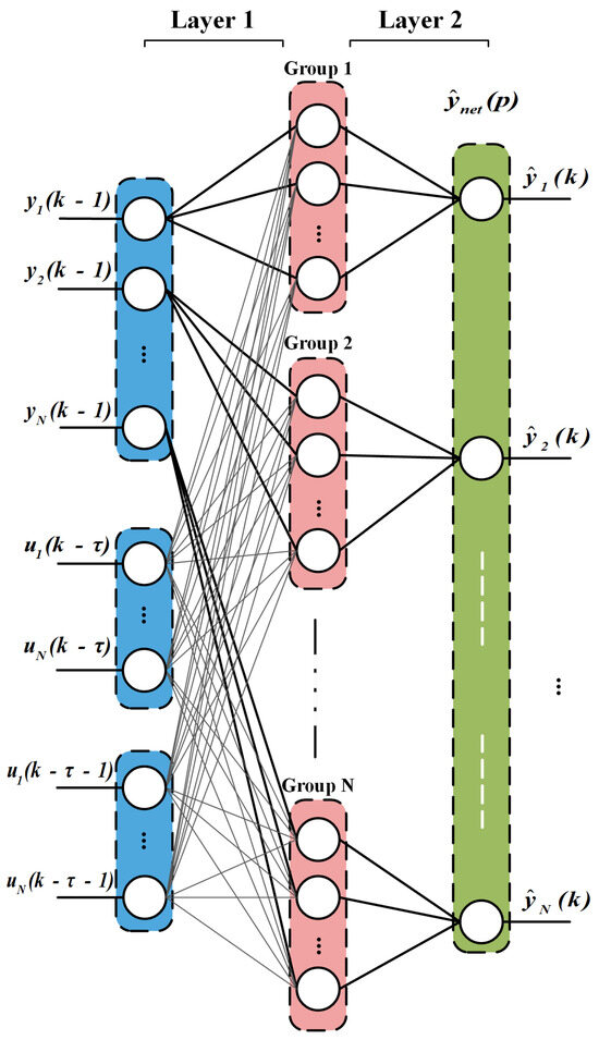
Figure 3.
Grouping neural network model for interaction multi−channel system identification. The hidden layer neurons are divided according to the number of channels.
According to Equation (5), the temperature change of each channel is related to and . Therefore, the temperature and current of each channel are used as input terms to the Grouping-NN, and the output is the predicted value of the temperature of all individual channels. The network’s output becomes a function of past inputs and outputs, which is given in Equation (10):
where is the current of the infrared heating device corresponding to channel N at the moment, and denotes the temperature value captured by channel N at moment .
The temperature at each measuring point is influenced by the nearby heaters, and the temperatures at other measuring points have little impact on it. As a result, during the neural network design process, the hidden layer neurons are categorized into N groups according to the channel number. Each group of neurons is linked to all the heater inputs but only to the measured input of this channel.
Due to the different connection, the weight matrix between the input layer and the hidden layer is split into and . indicates the weight matrix between the temperature input and the hidden layer, and denotes the weight matrix between current inputs and the hidden layer.
As the output of the Grouping-NN, indicates the predicted temperature of each channel. The weight matrix between the hidden layer and the output layer is denoted as v. and v need to perform Hadamard product operations with the sparse matrices during initialization and weight update.
The network’s mathematical operations are shown in Equations (11) and (12).
where is the output of the j-th node in hidden layer, is the activation function of the hidden nodes, is the output of the p-th node in the output layer, is the activation function of the output nodes, and q denotes the length of hidden layer. In this network, uses a linear activation function. The hidden layer activation function, , uses leakyReLU, shown in Equation (13).
where takes the value of 0.01.
The goal of the Grouping-NN is to find the optimal network weights to minimize the error between predicted and actual values. The loss function is computed independently for each channel, shown in Equation (14). The partial derivative of the loss function vector for is shown in Equation (15).
The network can be trained using the gradient descent method. The loss function is searched based on the negative gradient direction of the weight coefficients. The partial derivative of the loss function relative to the weights is found, so that the weights can be updated to obtain the global minimum of the error.
The gradient descent weight update method is shown in Equation (16).
where is the learning rate for the neural network training. According to the chain rule, of layer 1 could be expressed as:
Define as :
The weights of layer 2 can be expressed as:
The pseudocode of the Grouping-NN for multi-channel interaction system identification is shown in Algorithm 1 (the vectors in the code are all row vectors).
| Algorithm 1 Grouping-NN for Multi-Channel System Identification |
| 1: Initialization: Grouping-NN weights and ; 2: Initialization: sparse matrix and ; Input: Control data vector: ; Input: Measurement vector: Output: Weights matrix and ; Output: Estimated vector ; 3: while do 4: Normalised network input: ; 5: Layer 1 forward propagation: ; 6: Using activation function on hidden layer: ; 7: Layer 2 forward propagation with linear function: 8: Calculate the partial derivative of the loss function: 9: Backward propagating the err: 10: Update weights, the process needs to be multiplied by the sparse matrix and : 11: for range of j do 12: for range of p do 13: 14: end for 15: end for 16: for range of i do 17: for rang of j do 18: 19: end for 20: end for 21: Buffering the data and 22: ; 23: end while |
3.3. Grouping-NN-Based Smith Predictor
The Smith predictor is an effective method to solve the time-delay problem of the control system. The transfer function used in the Smith predictor is divided into the time-delay model and the system model without delay . In the temperature control system, the output of is compared with the measured temperature, then added to the output of , and the sum compensates the system input through a feedback loop. The accuracy of the transfer function greatly affects the control effectiveness. In practice, it is particularly difficult to estimate the transfer function of a real system, especially in an environment with interaction among multiple channels.
The Grouping-NN proposed in Section 3.2 can approximate the real multi-channel transfer function after training. Therefore, two Grouping-NNs, NN1 and NN2, are utilized to update the time-delay model and the system model without delay in the Smith predictor, which is shown in Figure 4. Here, presents the transfer function of the PID controller, and the heating system transfer function, , is divided into and time delay . and denote the transfer function and time delay in the Smith predictor, respectively.
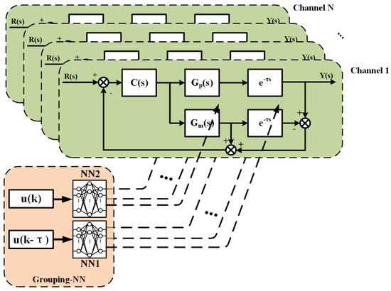
Figure 4.
Block diagram of the Grouping−NN−based multi−channel Smith predictor.
For the time-delay model, NN1 consists of the temperature input, , and the current input. The current inputs, , are values recorded by the buffer before the time delay, . The output of NN1 is compared with the temperature measured value and the differences are used for back propagation, which updates the weights during the control process.
For the system model without time delay, NN2 consists of the temperature input, , and the latest current input, . The output of NN2 is summed with the feedback values of the time-delay model. The weights of NN2 are provided by NN1.
The time-delay model and system model without delay in the Smith predictor share a common transfer function model, . If there is a deviation in the model, the deviation will be canceled out in two subtraction operations, so it is important to ensure that both subtraction operations use the same model. The proposed algorithm also retains this property, so that the same structure as well as the same weights are used in the computation of both Grouping-NNs. The NN2 network in the algorithm only performs forward propagation, and the weights are provided by the NN1. The weights are updated after both Grouping-NNs have been computed.
The pseudocode of the Grouping-NN-based Smith predictor is shown in Algorithm 2 (the vectors in the code are all row vectors).
| Algorithm 2 Grouping-NN-based Smith Predictor |
| 1: Initialization: PID parameters , , ; 2: Initialization: buffer of measurement data and control data Input: Measured vector ; Input: Reference vector ; Output: Controller output vector ; 3: while do 4: Using Algorithm 1 with input and with output NN1; 5: Using Algorithm 1 with input and with output NN2; 6: Updating neural network weights; 7: Calculate the predicted compensation: ; 8: Calculate the input vector of PID: ; 9: Calculate PID output using Equations (8) and (9); 10: Buffer PID outputs and measured values; 11: ; 12: end while |
4. Simulation
In this section, the proposed method is verified by system identification simulation. In addition, the performance of the proposed method in temperature control is evaluated by comparing it with traditional methods.
4.1. Preparation of Simulation
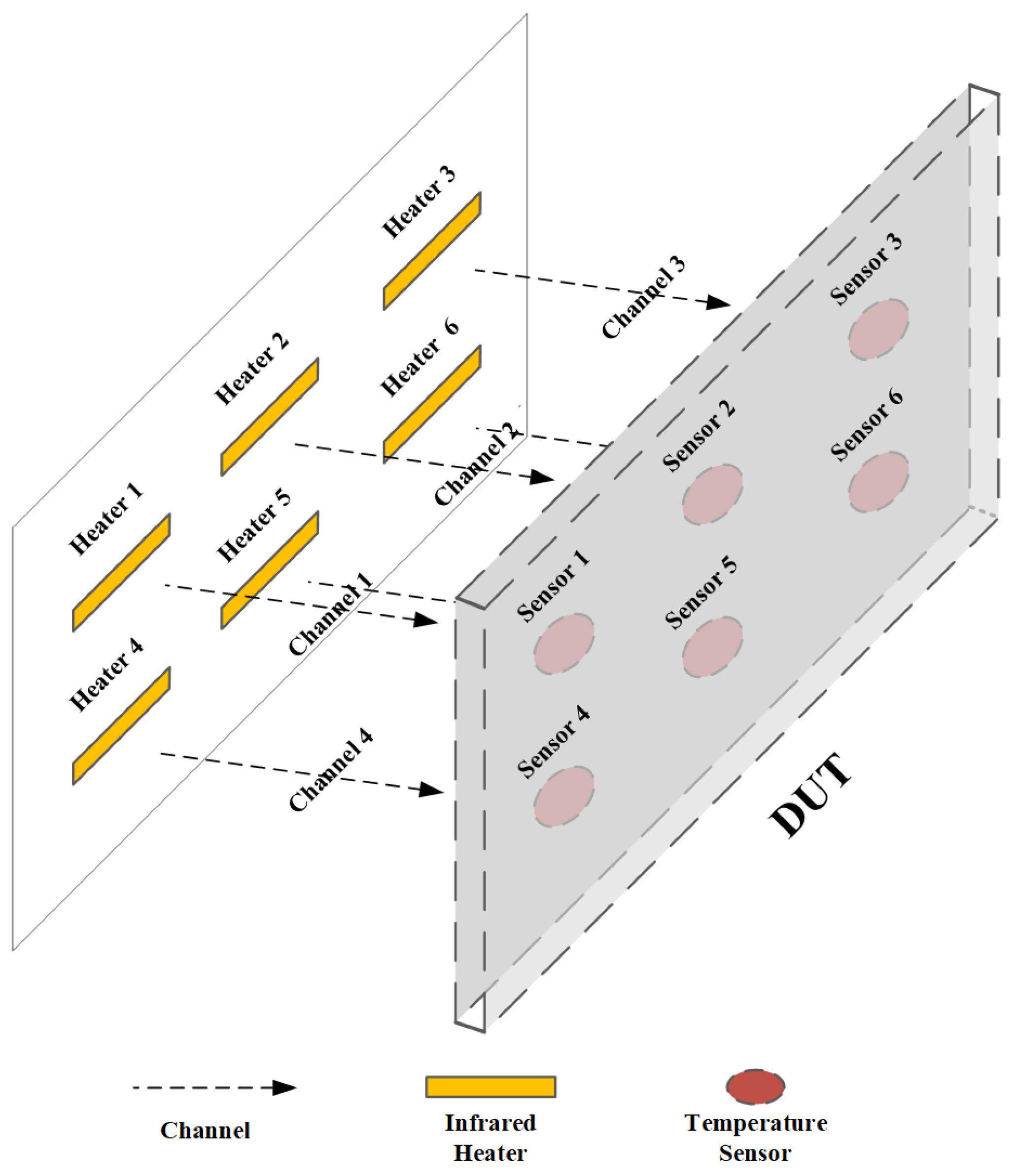
The simulation builds a 6-channel interaction heating model which includes six heaters and six sensors, shown in Figure 5. The heaters and sensors are all arranged in a arrangement. Each sensor forms a channel with a heater directly opposite it.
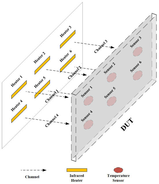
Figure 5.
Layout diagram of six channels for temperature control simulation.
When modeling, each sensor is assumed to be affected by adjacent heating units. The temperature calculations in the simulation are in the form of discrete difference equations. The temperature and current parameters of the transfer function in Equation (5) are expressed in matrix form as (22)–(24).
Here, is the coefficient vector of in the transfer function, and and denote the coefficients matrix of and in the transfer function.
The temperature model in the simulation is calculated by the matrix product, and the coefficient matrices are combined, as shown in Equation (25). The input matrix is shown in Equation (26).
The output of the transfer function is calculated in Equation (27).
where is the temperature vector containing the temperature output data from channel 1 to channel 6. The input matrix, , includes the temperature output at time and the current output with time delay. W denotes the Gaussian noise, where the mean is 0 and the variance is 0.02. The temperature model is calculated from the step response of each single heating device with different temperature sensors, and the multi-channel interaction transfer function is the accumulation of multiple FOPDT models.
To simulate the real situation, a saturator is added to the controller outputs, and is limited to [0,5]. In addition, the simulation programs are coded by Matlab R2020a in Windows 10, and the simulation is run on a computer with AMD R7 5800H and 16 GB of RAM.
4.2. Simulation Result of Identifier
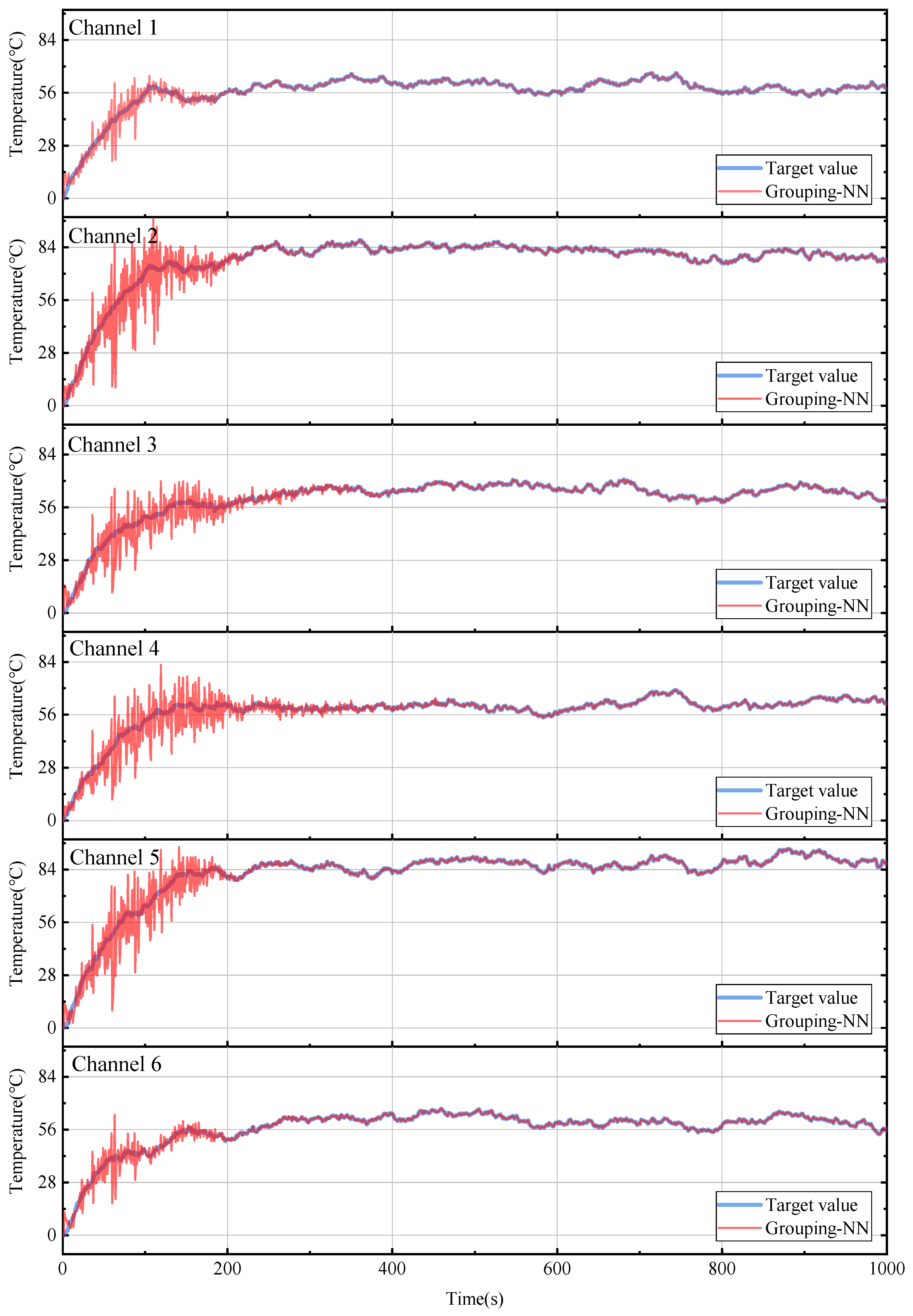
In this section, the Grouping-NN for multi-channel system identification is verified. Firstly, the generated random current is fed into the transfer function and the output temperature is calculated. Then, the current value before the time delay of 20 s and the temperature value at the previous moment are used as inputs to the Grouping-NN. Finally, the output of the network is compared with the calculated output of the transfer function. The results are shown in Figure 6, which presents the Grouping-NN’s training and identification process for all channels. The neural network iterates per second, and the horizontal axis in the graph indicates the time of the training process, and the vertical axis is the temperature of each channel. In the first 400 s of the simulation, the Grouping-NN is in the process of convergence and the estimation accuracy is insufficient. As time passes, the output of the Grouping-NN gradually approaches the output of the system model.
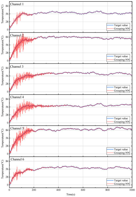
Figure 6.
Grouping−NN temperature system identification results in the simulation.
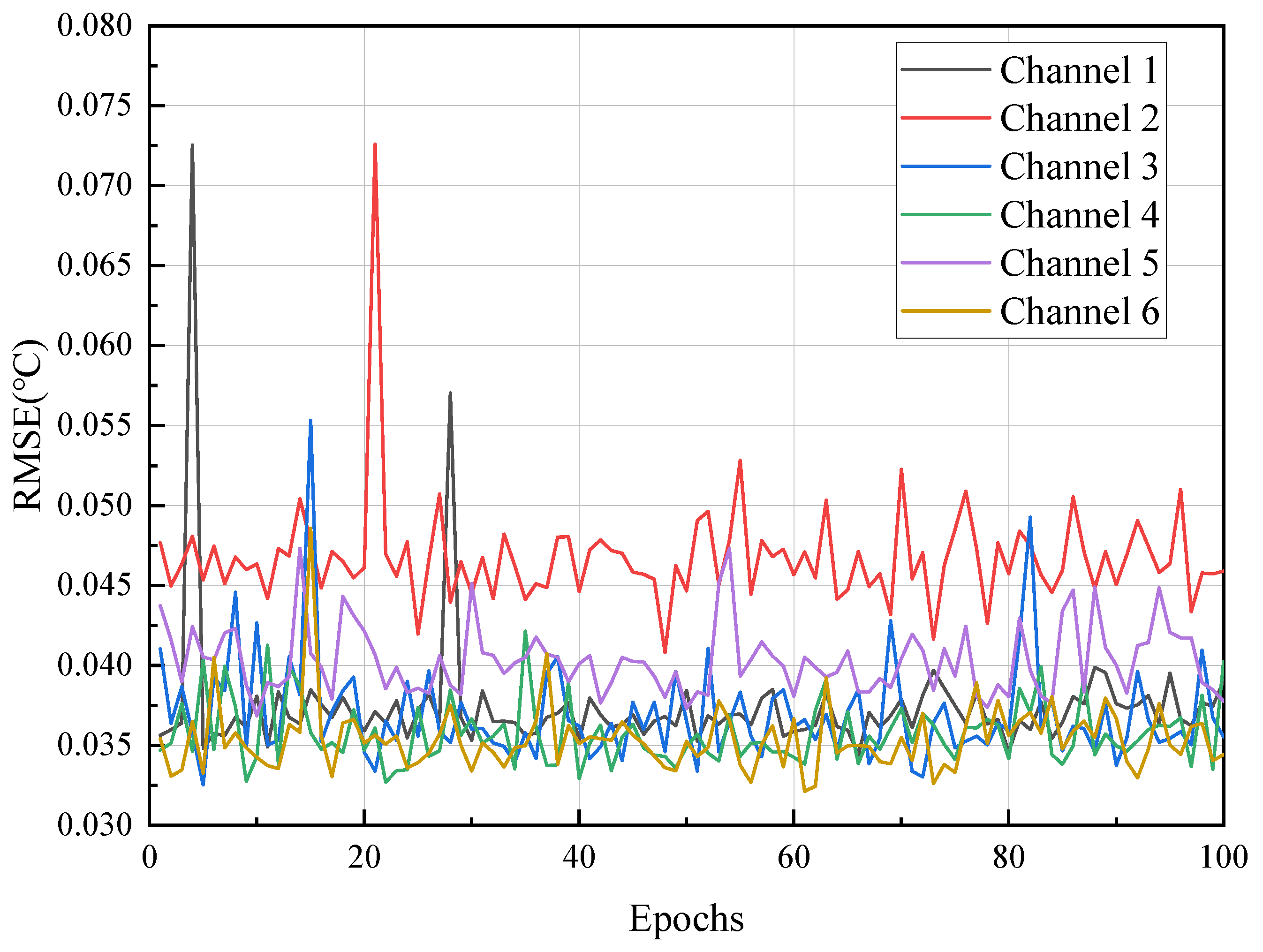
Further data statistics are performed to verify the accuracy of the proposed identification method. In the simulation, 100 rounds of system identification training are performed, and each round takes 1000 times of data after network convergence for statistics. The root mean square error (RMSE) is calculated by Equation (28).
where denotes the temperature value, indicates the estimated output of the Grouping-NN, N denotes the number of samples, and t is the time of network training. Figure 7 illustrates the temperature RMSE curves in 100 epochs for the trained Grouping-NN. Each epoch refers to the process in which the entire training dataset is trained by a neural network. This simulation result is used to verify the stability of the proposed Grouping-NN during the training process. As can be seen from the figure, the RMSE of the more-affected channels 2 and 5 is slightly larger than that of the others. All RMSEs do not exceed 0.075 °C, which confirms the effectiveness of the Grouping-NN in system identification.
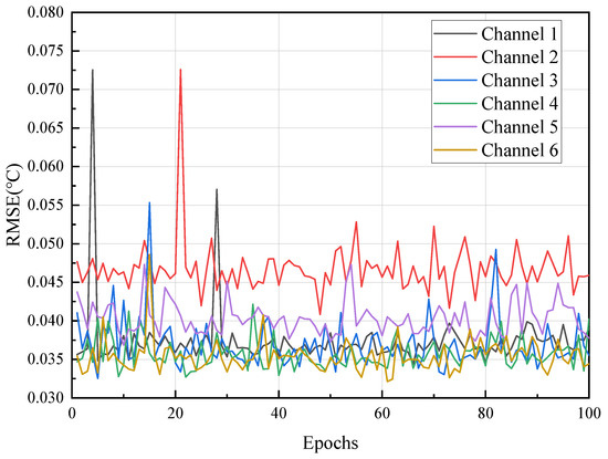
Figure 7.
The temperature RMSE of the Grouping−NN identifier in the simulation.
The performance metrics of the trained Grouping-NN for system identification are shown in Table 1. Avg denotes the mean value of RMSE for each channel.

Table 1.
The performance of multi-channel Grouping-NN identification method.
4.3. Simulation Result of Controller
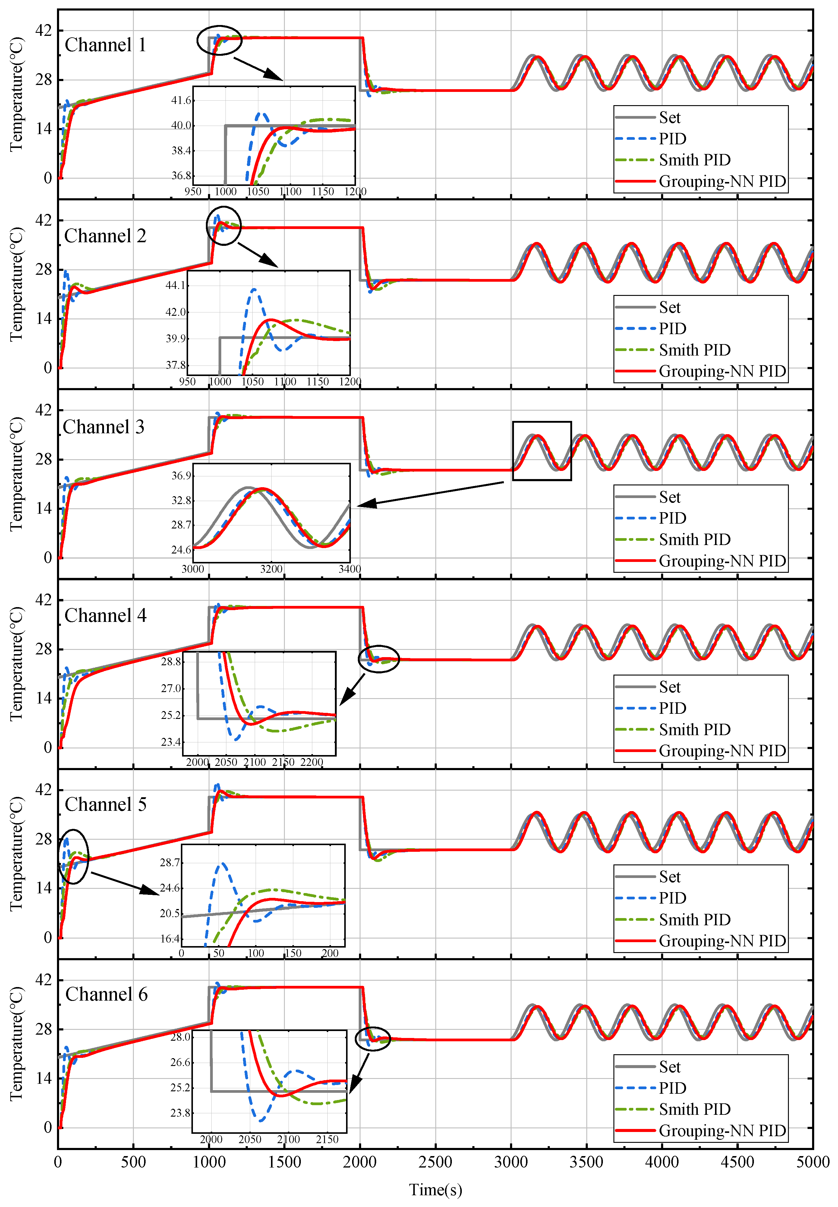
In this section, the trained Grouping-NN is combined with the Smith PID controller to perform temperature control tests. Six PID controllers are used to control six interaction channels, respectively. These controllers have the same coefficients of , , and . The set values of the temperature control are shown in Table 2, where indicates the target temperature and t is the time of the simulation. Under this setting, the temperature profile of each channel is plotted to compare the temperature results between the conventional PID, Smith PID, and Grouping-NN-PID, which is shown in Figure 8.

Table 2.
The set value of temperature control.
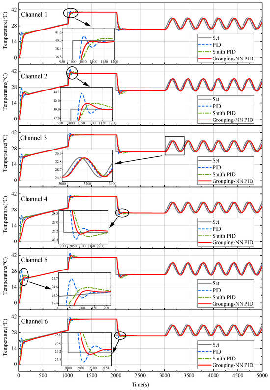
Figure 8.
Multi−channel temperature simulation results with different algorithms.
Overshoot is introduced to compare the performance of these controllers. Overshoot indicates the deviation between the maximum amplitude and the set value at that moment.
From the simulation curves, it can be seen that the overshoots of channel 2 and channel 5 are significantly larger than the other channels. According to positional relationships among these channels, channel 2 and channel 5 are indeed affected by other channels mostly.
The performances of each channel are given in Table 3. In condition 1, the different methods produce higher overshoots in channels 2 and 5 than in other channels. The PID controller has the largest overshoot of 8.112 °C, and the Smith PID controller has an overshoot of 3.144 °C. The maximum overshoot of the proposed method is only 1.997 °C, which is the minimum overshoot among these methods. The proposed method also outperforms the other methods in the cooling process in condition 3. These results demonstrate the control capability of the proposed method in a multi-channel interaction system.

Table 3.
The overshoot of interaction multi-channel control simulation (°C).
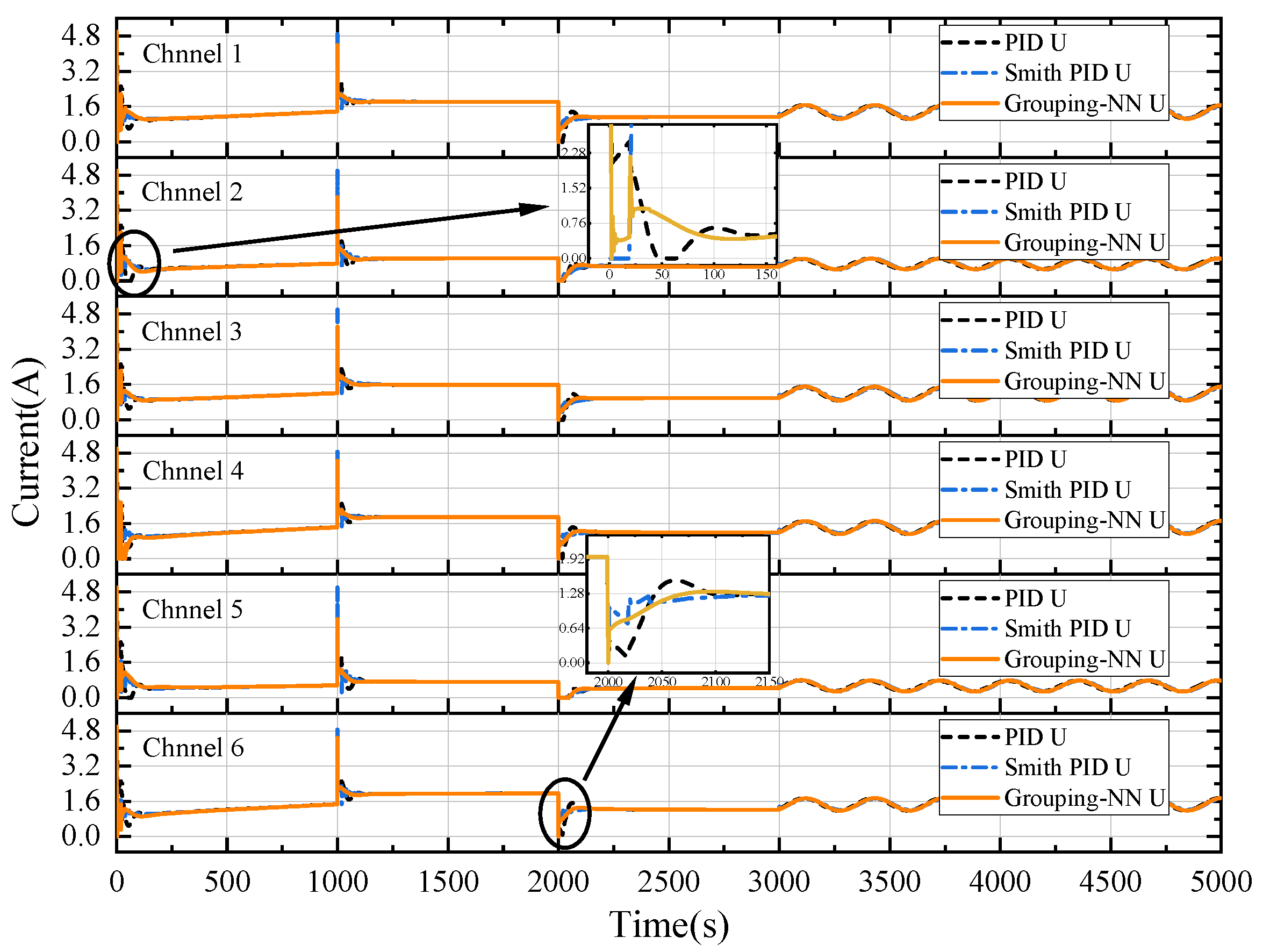
The PID controller acts on the object by outputting the current. The simulation records the current output of each controller, as shown in Figure 9, which is meant to provide a trend of the controller changes and to analyze the cause of the overshoot difference in Figure 8. From the current curves, it can be seen that the current changes of the PID and Smith PID controllers are more direct. Once the target temperature changes drastically, the output of the PID and Smith PID increases rapidly, which leads to a large overshoot. The proposed algorithm can adapt well through the Grouping-NN Smith predictor. It can be seen that the current callback time of the proposed method is earlier than the conventional controllers.
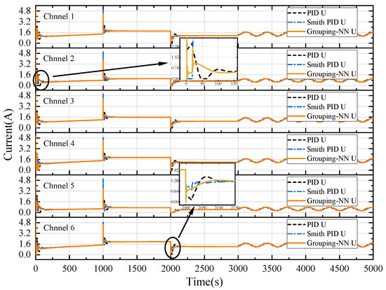
Figure 9.
Current output curves of each controller in the simulation.
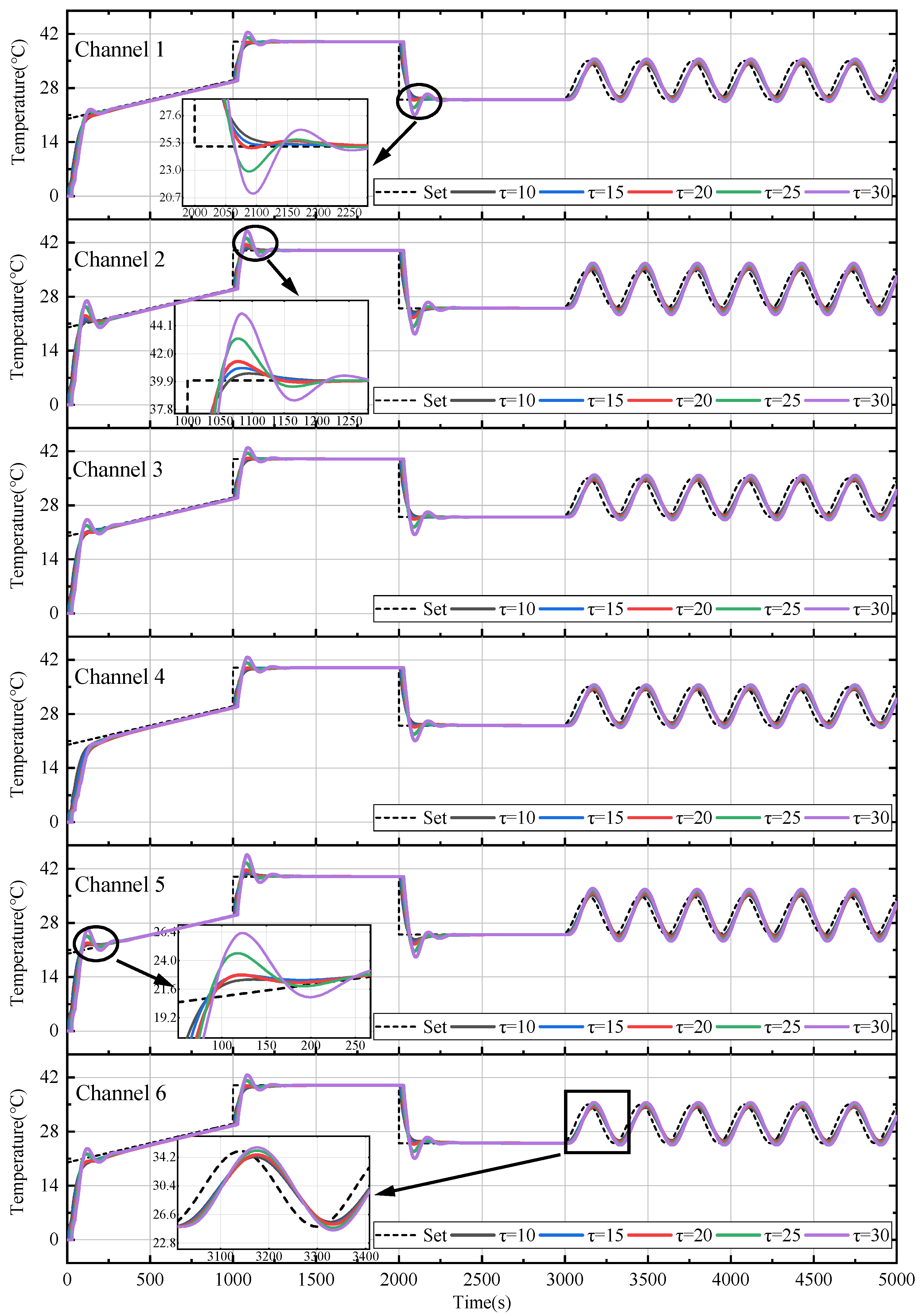
Even though the simulation transfer function is obtained based on the step response data of the actual TVT, it is likely that the actual system parameters are also different from the design parameters. Therefore, the control response of the proposed method is also verified in the simulation when the system parameter, , is changed. This simulation result is shown in Figure 10, and verifies the adaptability of the controller under uncertain parameters.
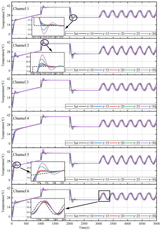
Figure 10.
Temperature simulation results with different time delays.
The simulation uses the same controller as before, and the red curve in the figure is the same as the temperature profile of the Grouping-NN PID in Figure 8. As can be seen from the figure, the system overshoots are similar for the time delay , and the overshoot and settling time are significantly large in the results for . The proposed controller has good adaptability for systems with a time delay that is less than the design requirements.
5. Experiment
In this section, the real thermal vacuum test is carried on for algorithm verification. The experiment settings and results are as follows.
5.1. Experiment Setting
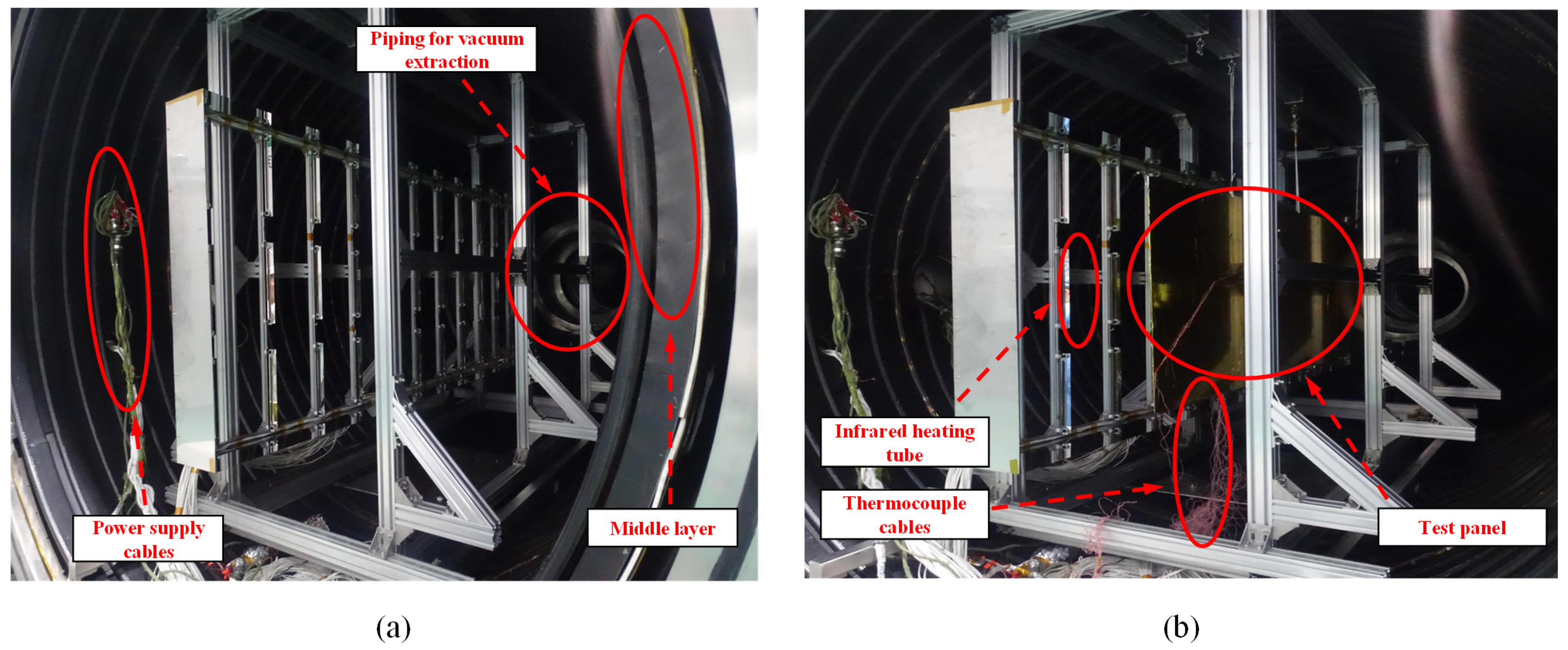
A temperature control system is set up in a TVC to validate the proposed algorithm. As the DUT, a 2.5 m × 1 m test panel is placed in the chamber. Six T-type thermocouples are attached to the surface of the DUT in a two-row and three-column layout. An array of infrared heating tubes are placed opposite to the DUT, and six of them directly opposite to the sensors are chosen as heaters for this experiment. The experimental scenario is shown in Figure 11.
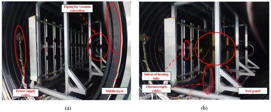
Figure 11.
Experimental scenario: (a) vacuum chamber, and (b) infrared heating system.
The infrared heating tubes are controlled by a programmable power supply outside the chamber, which is the N5750A, produced by Keysight Technologies, Inc. Thermocouples are connected to L4421A and 34465A for up to 40 channels of temperature acquisition. All devices above are connected to the host computer via an Ethernet switch. Based on the measured temperature, the proposed algorithm sends the calculated current values to the power supply for output. The experimental program is designed in C# language, running on a computer with a CPU of R7-5800H and a memory of 16 GB.
After the equipment is connected correctly, the chamber is closed and vacuumed. When the air pressure is less than Pa, liquid nitrogen is injected into the middle layer, which is arranged in multiple spiral pipes to provide heat sink for the test. Meanwhile, the temperature control program is started to stabilize the temperature at 20 °C and prepare for the test.
5.2. Experiment Results and Analysis
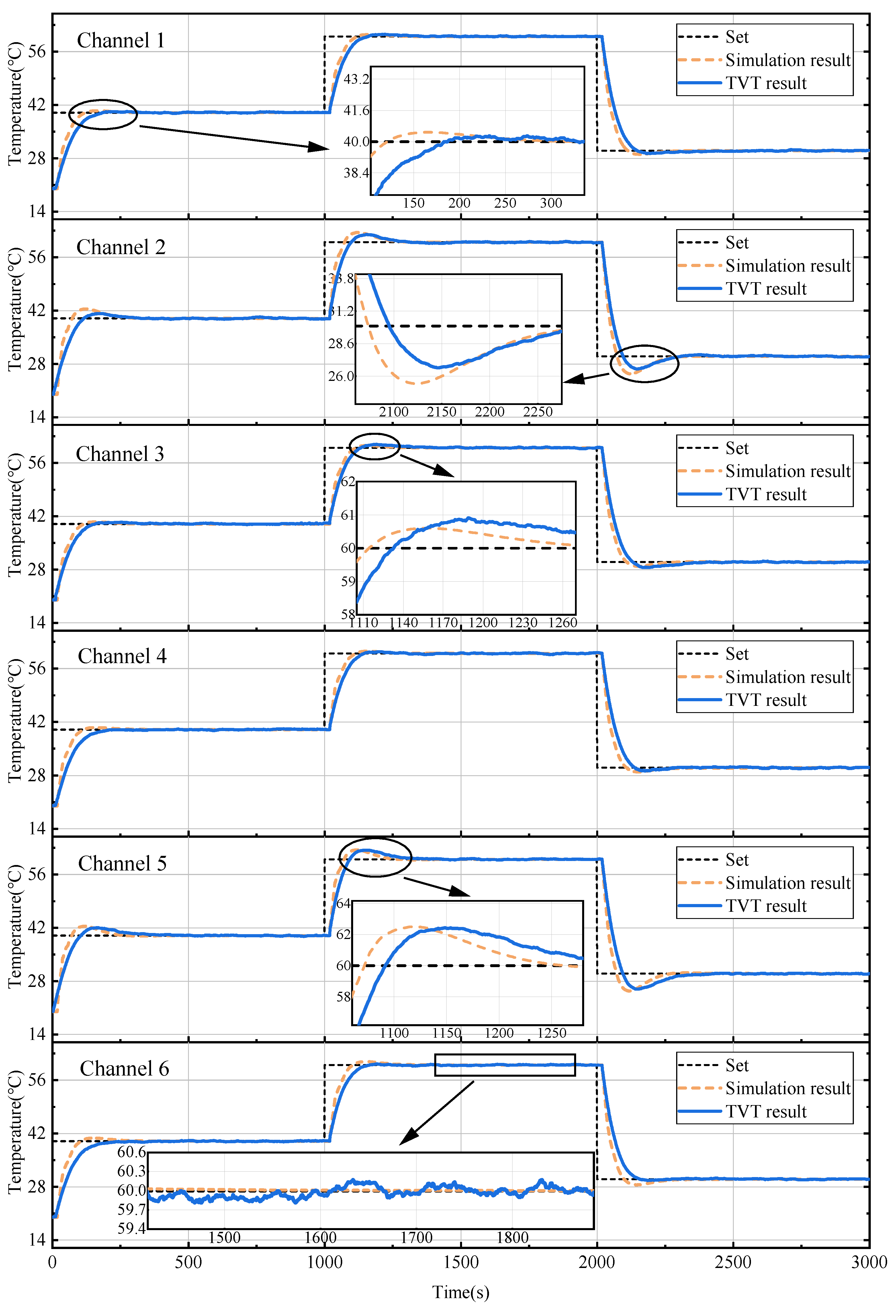
The program is started to validate the proposed algorithm when the DUT temperature stabilizes at 20 °C, and the moment is marked as 0 s. In condition 1, the temperature is set to 40 °C and stabilized for a period of time to 1000 s. Then, in condition 2, the temperature is set to 60 °C, stabilized, and maintained to 2000 s. In condition 3, the temperature is set to 30 °C to the end of the test. The acquisition interval and control interval of this experiment are set at 1 s.
Figure 12 shows the curves of temperature changing with time for the trained Grouping-NN PID algorithm. In order to provide a better comparison between the simulation and experimental results, the simulation curves with the same set value are also added to the figure. According to the detailed zoomed-in graph, it can be seen that, in the actual TVT, the more-affected channels 2 and 5 have a lower time delay and a faster temperature rising speed compared with the simulation results. Although there is a certain deviation between the experimental curve and the simulation curve, the temperature control trend is similar, proving the effectiveness of the simulation. The corresponding performance characteristics of the TVT result are shown in Table 4, Table 5, Table 6 and Table 7. The control time, settling time, and steady-state error are introduced to show the performance of the proposed controller. The control time indicates the time taken from 10% to 90% of the steady-state value. The settling time means the time taken from the start value to the maximum error under 0.2 °C. The steady-state error is the RMSE value after settlement.
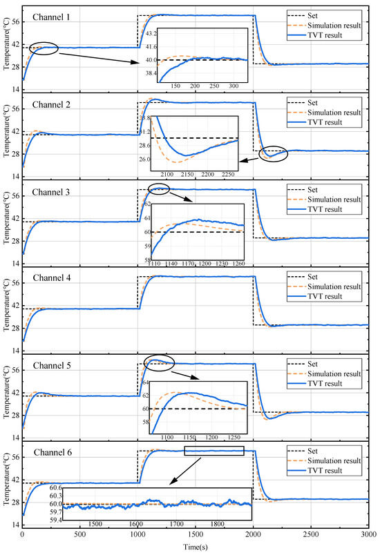
Figure 12.
The comparison of simulation and experimental results.

Table 4.
The overshoot of the experiments.

Table 5.
The steady-state error of the experiments.

Table 6.
The settling time of the experiments.

Table 7.
The rise time of the experiments.
Channel 2 and channel 5 have the largest overshoot, with a maximum overshoot of 2.42 °C during the heating process. For other channels, the overshoots are mostly below 0.5 °C. The settling time of each channel is within 370 s, and the channel with less disturbance stabilizes faster than the others. For the control time, channel 2 and channel 5 are the fastest, with just 70–91 s. The steady-state error is mainly affected by the external environment, and the average error of each channel is about 0.1 °C.
After verification, the proposed method can work effectively in practical control. The overshoot is small and the temperature does not oscillate when reaching the set value. All performances satisfy the requirements of the thermal vacuum test.
6. Conclusions
In this paper, a Grouping-NN interaction identification-based Smith PID controller is proposed. By grouping the neurons in the hidden layer, the irrelevant connections of the network are reduced and the convergence speed is increased. Two Grouping-NNs are used to update and of the Smith predictor, improving the accuracy of the Smith PID controller. After simulation verification, the Grouping-NN can estimate the system model in real time and accurately. By comparing with the PID and Smith PID, the proposed method has less overshoot and a shorter settling time. In the practical experiment, the overshoot can meet the requirements of the TVT. In summary, the proposed method can estimate the model of each channel in real time under a multi-channel interaction scenario. The hidden layer neurons grouping method can effectively reduce the disturbance of the temperature input. The Grouping-NN can update the transfer function in the Smith predictor to improve the multi-channel control effect. This method can identify the temperature relationship among multiple channels, which is the basis of multi-channel uniform control. The Grouping-NN not only serves as a key for multi-channel simulation modeling in subsequent studies, but also provides more options for optimizing the multi-channel controller. Subsequently, we will optimize the temperature uniformity in a multi-channel thermal vacuum test, hoping to minimize the temperature gap between the measurement points of the DUT.
Author Contributions
Conceptualization, F.L.; methodology, F.L. and L.Y.; software, L.Y. and A.Y.; validation, F.L., L.Y. and A.Y.; formal analysis, Z.Z.; investigation, F.L.; resources, F.L.; data curation, L.Y. and B.S.; writing—original draft preparation, F.L. and L.Y.; writing—review and editing, F.L., Z.Z. and B.S.; visualization, L.Y. and A.Y.; supervision, F.L., Z.Z. and B.S.; project administration, F.L., Z.Z. and B.S.; funding acquisition, F.L. All authors have read and agreed to the published version of the manuscript.
Funding
This research was funded by Beijing Natural Science Foundation, grant number 3164043.
Data Availability Statement
The data presented in this study are available on request from the corresponding author.
Conflicts of Interest
The authors declare no conflicts of interest.
References
- Zhang, J.; Xie, J.H.; Wang, Y.R. The application and the development trend of the measurement and control system in the spacecraft vacuum thermal test. Spacecr. Environ. Eng. 2012, 29, 263–267. [Google Scholar]
- Almeida, J.S.; Santos, M.B.; Panissi, D.L.; Garcia, E.C. Effectiveness of low-cost thermal vacuum tests of a micro-satellite. Acta Astronaut. 2006, 59, 483–489. [Google Scholar] [CrossRef]
- Salleh, N.; Daud, S.M.; Sabri, S.F.; Ahmad@Salleh, N.A.; Adam, M.Z. Enhancing Temperature Control Method of Thermal Vacuum Chamber for Satellite Testing Using Optimization Algorithm: A Review. J. Teknol. 2016, 78, 5–7. [Google Scholar] [CrossRef][Green Version]
- Elshaer, A.M.; Soliman, A.; Kassab, M.; Hawwash, A. Experimental and numerical investigations of an open-cell copper foam (OCCF)/phase change material (PCM) composite-based module for satellite avionics thermal management in a thermal vacuum chamber (TVC). J. Energy Storag. 2024, 75, 109572. [Google Scholar] [CrossRef]
- Werkhausen, A.D.; Hey, H. Temperature transition optimization in cryogenic systems: Application to liquid nitrogen expenditure reduction in a thermal vacuum chamber case study. Appl. Therm. Eng. 2024, 236, 121863. [Google Scholar] [CrossRef]
- Jang, B.; Lee, W.; Lee, J.J.; Jin, H. Artificial neural network-based temperature prediction of a lunar orbiter in thermal vacuum test: Data-driven reduced-order models. Aerosp. Sci. Technol. 2024, 145, 108867. [Google Scholar] [CrossRef]
- Zhang, X.; Wu, L.; Liu, H.; Feng, J.; Xu, M.; Cheng, R. Research and Verification of Multi-Satellite Thermal Vacuum Test Method. In Proceedings of the 2020 International Conference on Sensing, Measurement & Data Analytics in the era of Artificial Intelligence (ICSMD), Xi’an, China, 15–17 October 2020; pp. 347–351. [Google Scholar] [CrossRef]
- Park, S.; Kim, S. Nonlinear Model Predictive Control of Thermal Vacuum Chamber Temperature. Int. J. Aeronaut. Space Sci. 2023, 25, 213–228. [Google Scholar] [CrossRef]
- Guo, J.-C.; Li, F.-Y.; Chen, A.-R.; Zhang, L.-H.; Liu, S.-W. Automatic Temperature Control Design for Thermal Vacuum Tests Based on Fuzzy PID Control. In Proceedings of the 2019 International Conference on Quality, Reliability, Risk, Maintenance, and Safety Engineering (QR2MSE), Zhangjiajie, China, 6–9 August 2019; pp. 186–194. [Google Scholar]
- Zhan, H.; Sun, Y.; Liu, D.; Liu, H. Adaptive neural network PID controller design for temperature control in vacuum thermal tests. In Proceedings of the 2016 Chinese Control and Decision Conference (CCDC), Yinchuan, China, 28–30 May 2016; pp. 458–463. [Google Scholar] [CrossRef]
- Ziegler, J.G.; Nichols, N.B. Optimum settings for automatic controllers. Trans. Am. Soc. Mech. Eng. 1942, 64, 759–765. [Google Scholar] [CrossRef]
- Liu, Z.; Liu, Z.; Liu, J.; Wang, N. Thermal management with fast temperature convergence based on optimized fuzzy PID algorithm for electric vehicle battery. Appl. Energy 2023, 352, 121936. [Google Scholar] [CrossRef]
- Han, S.Y.; Dong, J.F.; Zhou, J.; Chen, Y.H. Adaptive Fuzzy PID Control Strategy for Vehicle Active Suspension Based on Road Evaluation. Electronics 2022, 11, 921. [Google Scholar] [CrossRef]
- Abdelwanis, M.I.; El-Sousy, F.F.M.; Ali, M.M. A Fuzzy-Based Proportional Integral Derivative with Space-Vector Control and Direct Thrust Control for a Linear Induction Motor. Electronics 2023, 12, 4955. [Google Scholar] [CrossRef]
- Ding, Y.; Ren, X.; Zhang, X.; Liu, X.; Wang, X. Multi-Phase Focused PID Adaptive Tuning with Reinforcement Learning. Electronics 2023, 12, 3925. [Google Scholar] [CrossRef]
- Huang, H.; Zhang, S.; Yang, Z.; Tian, Y.; Zhao, X.; Yuan, Z.; Hao, S.; Leng, J.; Wei, Y. Modified Smith fuzzy PID temperature control in an oil-replenishing device for deep-sea hydraulic system. Ocean. Eng. 2018, 149, 14–22. [Google Scholar] [CrossRef]
- Feliu-Batlle, V.; Rivas-Perez, R. Control of the temperature in a petroleum refinery heating furnace based on a robust modified Smith predictor. ISA Trans. 2021, 112, 251–270. [Google Scholar] [CrossRef] [PubMed]
- Pan, Y.; Xie, J.; Zhang, C.; Zhu, X.; Zhao, P. High efficiency far-infrared barrel heating control with excess heat prediction based on generalized predictive control in injection molding. Int. J. Heat Mass Transf. 2024, 218, 124756. [Google Scholar] [CrossRef]
- Xu, L.; Chen, L.; Xiong, W. Parameter estimation and controller design for dynamic systems from the step responses based on the Newton iteration. Nonlinear Dyn. 2015, 79, 2155–2163. [Google Scholar] [CrossRef]
- Tutunji, T.A. Parametric system identification using neural networks. Appl. Soft Comput. 2016, 47, 251–261. [Google Scholar] [CrossRef]
- Hagiwara, T.; Yamada, K. A design method of modified PID controllers for multiple-input/multiple-output plants. IFAC Proc. Vol. 2008, 41, 5825–5830. [Google Scholar] [CrossRef]
- Hagiwara, T.; Yamada, K.; Ando, Y.; Murakami, I.; Aoyama, S.; Matsuura, S. A design method for modified PID control systems for multiple-input/multiple-output plants to attenuate unknown disturbances. In Proceedings of the 2010 World Automation Congress, Kobe, Japan, 28–30 May 2010; pp. 1–6. [Google Scholar]
- Gopmandal, F.; Ghosh, A. LQR-based MIMO PID control of a 2-DOF helicopter system with uncertain cross-coupled gain. IFAC-PapersOnLine 2022, 55, 183–188. [Google Scholar] [CrossRef]
- Carlucho, I.; De Paula, M.; Acosta, G.G. An adaptive deep reinforcement learning approach for MIMO PID control of mobile robots. ISA Trans. 2020, 102, 280–294. [Google Scholar] [CrossRef]
- Ahmad, M.A.; Azuma, S.-I.; Sugie, T. Performance analysis of model-free PID tuning of MIMO systems based on simultaneous perturbation stochastic approximation. Expert Syst. Appl. 2014, 41, 6361–6370. [Google Scholar] [CrossRef]
- Boyd, S.; Hast, M.; Strm, K.J. MIMO PID tuning via iterated LMI restriction. Int. J. Robust Nonlinear Control. 2016, 26, 1718–1731. [Google Scholar] [CrossRef]
- Wang, Y.; Ding, F. Novel data filtering based parameter identification for multiple-input multiple-output systems using the auxiliary model. Automatica 2016, 71, 308–313. [Google Scholar] [CrossRef]
Disclaimer/Publisher’s Note: The statements, opinions and data contained in all publications are solely those of the individual author(s) and contributor(s) and not of MDPI and/or the editor(s). MDPI and/or the editor(s) disclaim responsibility for any injury to people or property resulting from any ideas, methods, instructions or products referred to in the content. |
© 2024 by the authors. Licensee MDPI, Basel, Switzerland. This article is an open access article distributed under the terms and conditions of the Creative Commons Attribution (CC BY) license (https://creativecommons.org/licenses/by/4.0/).

