A Method for Assessing the Degradation of PVC-Insulated Low-Voltage Distribution Cables Exposed to Short-Term Cyclic Aging

Abstract

The distribution grid comprises cables with diverse constructions. The insulating material used in low-voltage (LV) distribution cables is predominantly PVC. Furthermore, the presence of cables with different structures in the grid poses challenges in detecting the aging of the cable network. Finding a universal and dependable condition-monitoring technique that can be applied to various types of cables is indeed a challenge. The diverse construction and materials used in different cables make it difficult to identify a single monitoring approach that can effectively assess the condition of all cables. To address this issue, this study aims to compare the thermal aging behavior of different LV distribution cables with various structures, i.e., one cable contains a PVC belting layer, while the other contains filler material. The growing adoption of distributed generation sources, electric vehicles, and new consumer appliances in low-voltage distribution grids can lead to short, repetitive overloads on the low-voltage cable network. Hence, these cable samples were exposed to short-term cyclic accelerated aging in the climate chamber at 110 °C. The cable’s overall behavior under thermal stress was evaluated through frequency and time domain electrical measurements (including tan $\delta$ and extended voltage response) and a mechanical measurement (Shore D). The tan $\delta$ was measured in the frequency range of 20 Hz–500 kHz by using the Wayne-Kerr impedance analyzer. The extended voltage response measurement was conducted using a C# application developed in-house specifically for laboratory measurements in the .NET environment. The study observed a strong correlation between the different measurement methods used, indicating that electrical methods have the potential to be adopted as a non-destructive condition-monitoring technique.

1. Introduction

The threat of global warming continues to loom over the planet, with the greenhouse effect playing a significant role in driving this phenomenon [1,2]. A key aspect of reducing the greenhouse effect involves transitioning away from fossil fuels as the primary energy source and, instead, embracing renewable sources [3]. The term energy transition refers to reducing conventional energy production and increasing renewable sources like solar and wind [4]. As renewable power plants expand, electricity distribution is shifting towards a decentralized model known as distributed generation [5,6]. Unlike the traditional centralized grid approach, this model divides the network into smaller-scale grids. In the smart grid concept, these smaller grids can operate independently and feed excess generation back into the main grid [7,8]. Power cables play an essential role in this transition and the future of the energy supply system. However, the existing power distribution networks were built several decades ago, and increasing distributed generation presents new challenges to the infrastructure [9]. These challenges include cyclic loads, unbalanced loads, and voltage pulses caused by inverters on low-voltage (LV) cable networks [10]. Furthermore, the occurrence of heatwaves is on the rise due to climate change. This trend is expected to intensify in the coming years due to global warming. This phenomenon contributes to many power system failures, especially in urban areas [11]. On a typical hot summer day, the failure rate of joints increases [12]. These factors can lead to insulation degradation and pose a risk to the integrity of the cables [13]. This degradation, known as insulation aging, refers to the irreversible deterioration of material properties caused by external environmental factors such as heat, radiation, moisture, and electric fields. These factors can result in chemical changes, the evaporation of plasticizers and additives, and the formation of new molecular chains [14,15]. The aging of dielectric materials has a negative impact on their insulation properties and can ultimately lead to electrical breakdown. As a result, condition monitoring (CM) has become a prominent research topic in this field [16]. In addition to various condition-monitoring (CM) techniques based on physical measurements, recent proposals by authors have leaned towards using machine learning to forecast failures. Atringa et al. highlighted that joints are the most susceptible components of distribution networks, accounting for 80% of all failures between 2015 and 2020. They implemented a machine learning methodology to anticipate power outages caused by heatwaves [11].

In general, accelerated aging tests are commonly conducted to estimate the lifetime of insulating materials used in power cables [17]. These tests typically involve exposing the materials to prolonged periods of increased temperatures. However, in the actual cable lines, the insulation is subjected to thermal cycling due to cyclic loads, which introduces additional stress and triggers degradation mechanisms that are not simulated in standard thermal aging tests [18]. While constantly elevated temperature tests provide valuable insights into the long-term behavior of insulating materials, they do not fully replicate the real-life conditions experienced by cables in operation. The thermal stress resulting from cyclic loads can lead to additional degradation mechanisms, such as thermal expansion and contraction, which can accelerate the aging process of the insulation [19]. Traditional, accelerated aging tests, conducted at a constant temperature, do not adequately capture these mechanisms [18]. Two primary degradation processes occur when plasticized PVC is exposed to high temperatures. These are dehydrochlorination and the loss of the plasticizer [20]. Dehydrochlorination is the removal of hydrogen and chlorine atoms from the PVC polymer chain. This process leads to the formation of double bonds and the release of hydrogen chloride gas [21]. On the other hand, there is the loss of the plasticizer, which is a substance added to PVC to improve its flexibility and processability [22]. At high temperatures, the plasticizer molecules can evaporate or migrate out of the PVC matrix, resulting in plasticizer loss, which can decrease the flexibility and mechanical properties of the PVC material. At lower temperatures, the primary degradation mechanism observed in plasticized PVC is the loss of plasticizers [20,23,24].

The distributed sources are usually connected to the low-voltage cable network [25], which contains various cables with different constructions. However, PVC is most commonly used as the insulating material in LV distribution cables [26,27,28]. Multiple factors influence the degradation of the insulating material, and the diverse cable structures make it challenging to detect aging on the cable network. However, knowing the correct condition could optimize cable replacements in the network [29]. In the case of low-voltage power cables, the most common cause of failure is water ingress through the damaged jacket [30]; therefore, one of the most important condition characteristics is the jacket’s mechanical integrity. Several techniques can measure the mechanical characteristics of cable insulation; nevertheless, these test methods are destructive because samples must be taken from the cable [31]. Hence, several studies have investigated the correlation between the mechanical and dielectric properties of the polymeric components of low-voltage cables. For example, in the case of widely used ethylene propylene rubber (EPR) and cross-linked polyethylene (XLPE), the dissipation factor and the imaginary permittivity measured in the kHz and MHz range, typically 100 kHz, correlate well with the mechanical properties [32,33,34,35]. But, in the case of different cable structures (e.g., non-shielded XLPE-insulated and CSPE-jacketed cable) and the two different insulating materials necessarily only being able to be measured together, other frequencies of dielectric spectrum, e.g., 100 Hz, correlate with the mechanical properties [36]. In the low-voltage distribution grid, different cables with different structures are usually used even in the same cable line, making the dielectric-measurement-based condition testing more difficult because the various cable components affect the dielectric properties differently [37]. Consequently, it is imperative to identify a non-destructive method that can be universally applied to low-voltage PVC cables in the distribution grid.

To address this issue, this study aims at comparing the thermal aging behavior of different LV distribution cables with various designs. Correlation analysis aims to find a common aging marker and a reliable non-destructive CM technique that can be applied for both cable types. Two PVC-insulated LV cable specimens, SZRMtKVM- and NYCWY-type, with different structures and cross-sections, were prepared and subjected to short-term cyclic thermal stress in a climate chamber. The dielectric parameters, specifically tan $\delta$, were measured after each aging round using a frequency range of 20 Hz to 500 kHz. Furthermore, the decay and return voltage slopes ($S_d$, $S_r$) were measured via extended voltage response (EVR) as the time domain spectroscopy (TDS) measurement. Last but not least, the mechanical measurement was performed with a Shore D hardness tester. The correlation between all the dielectric parameters and the hardness was analyzed. The results presented in this paper serve as a solid foundation for finding common condition-monitoring systems for different types of cables in the grid.

Section 2 presents the methodology and materials used in this research. Section 3 gives an overview of the results obtained. Section 4 provides the analysis of the results obtained from the measurements, and finally, Section 5 is the conclusion, where the main findings are summarized.

2. Materials and Methods

Two different LV cable samples with different geometries were exposed to cyclic thermal stress. The study examined how thermal stress affects the dielectric and mechanical parameters by utilizing frequency domain spectroscopy, including tan $\delta$, and extended voltage response measurements in the time domain. Lastly, the hardness of the jacket was evaluated using the Shore D method.

2.1. Sample Types

A total of six specimens were prepared from two PVC-insulated LV cables to find a general dielectric-measurement-based condition monitoring technique:

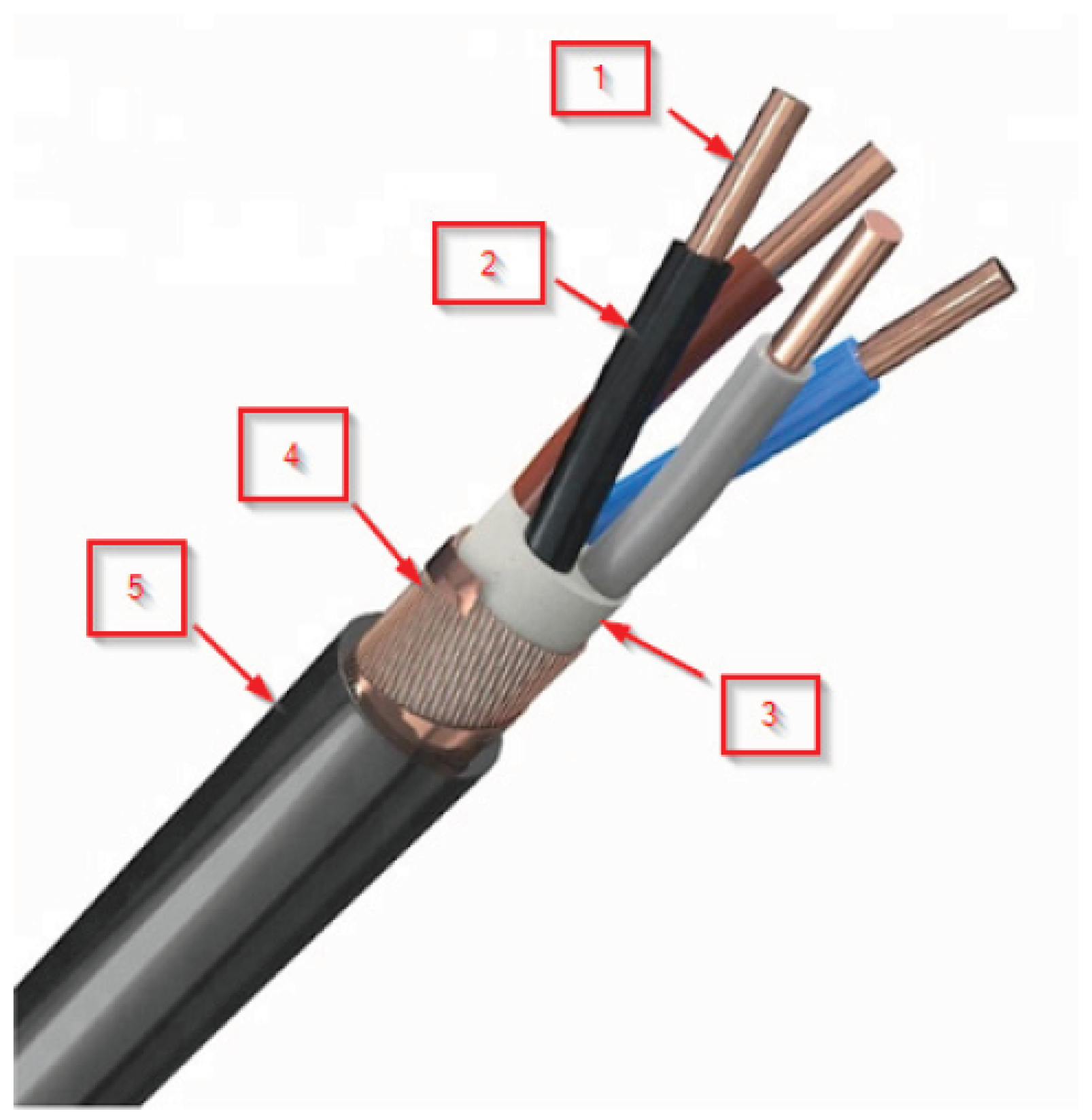
• NYCWY $0.6/1$ kV $4\times 10$ mm², manufactured by Cablel Hellenic Cables Group. The structure from inside to outside: 1. copper conductors, 2. PVC core insulation, 3. filling material, 4. copper wire and tape screen, and 5. PVC jacket. The cable structure of the NYCWY type can be seen in Figure 1. The maximum conductor operating temperature of NYCWY is 70 °C.
• SZRMtKVM $0.6/1$ kV $4\times 6$ mm², manufactured by Pyrismian MKM Kft. The structure from inside to outside: 1. copper conductors, 2. PVC core insulation, 3. PVC tape belt, 4. steel armor, and 5. PVC jacket. The cable structure of SZRMtKVM can be seen in Figure 2. According to the datasheet, the maximum conductor operating temperature of SZRMtKVM is 70 °C.

2.2. Aging

Three cable samples from each group were exposed to accelerated cyclic thermal aging. The aging temperature was 110 °C, and the duration was 3 or 6 h per round. A total aging time of eighteen hours was achieved. As shown in other studies presented in the literature, which utilized 18 h or even longer aging times, the initial behavior of aging exhibits a non-uniform trend; for instance, Shore D hardness decreases after the first aging cycle and, then, increases in subsequent cycles [38,39]. This study also observed that the aging behavior is uniform in later cycles, as evidenced by the consistent trend observed towards 18 h. The steps of one aging round were as follows:

• Setting the climate chamber temperature to 110 °C.
• Placing the samples inside the climate chamber once the temperature reached the setpoint value.
• Keeping the samples inside the climate chamber for accelerated thermal aging.
• Removing the samples from the climate chamber.
• Placing the samples at room temperature for pre-conditioning for 24 h.
• Performing the dielectric measurements.

According to IEC 60502-1, thermal aging should be carried out at least 10 $\pm 2$ °C more than the maximum conductor temperature, which is 70 °C during normal operation and 160 °C during short-circuit operation [40]. The temperature for thermal aging was set to 110 °C. This temperature was chosen for easier comparison with previous studies and was intended to use a temperature higher than specified in the standard.

2.3. Measurement Techniques

2.3.1. Dielectric Response Measurement

The dielectric response (DRM) is an extensively beneficial CM technique that researchers in the field use [41]. It is based on measuring the current that flows through the tested dielectric when it is excited by voltage. The measured current is recorded in the time domain if the tested insulation is excited by DC voltage. However, in the case of AC voltage, the amplitude and phase of the current are assessed across a wide frequency spectrum. DRM is used to monitor the degradation of LV cables [42].

• Tan $\delta$ Measurement

When a sample under testing is subjected to AC voltage, the ratio of the resistive and capacitive currents flowing through the insulation is referred to as tan $\delta$. It is a non-destructive CM technique, and it assesses the dielectric loss of insulation. Therefore, it is an extensively used method [43]. It is used for describing the losses in the dielectric. A Wayne-Kerr 6430A impedance analyzer, shown in Figure 3, was utilized for measuring tan $\delta$ in the frequency domain from 20 Hz to 500 kHz.

The cable sample was wrapped with aluminum foil to create a conductive surface on the jacket. Since the cable samples were multi-core, the cores and tape screens were short-circuited. One probe from the measuring device was connected to the jacket, and the other was connected to the rest, as seen in Figure 4.

• Extended voltage response (EVR)

This measurement technique is based on charging and discharging the dielectric by applying a constant DC voltage. It measures the decay and return voltage slopes. The decay voltage slope ($S_d$) is measured once the charging period ($t_{ch}$) finishes. On the other hand, the return voltage slope ($S_r$) is measured after a few seconds of shorting ($t_{dch}$). $S_d$ is directly proportional to the conductivity, while $S_r$ is directly proportional to the polarization conductivity. The classic voltage response (VR) measurement was extended with multiple discharging points. Multiple discharging times allow for investigating different polarization processes [44]. Having a long discharging time allowed us to investigate slow polarization processes like interfacial, bulk, and hopping polarizations [45].

The VR and EVR timing diagrams can be seen in Figure 5. The usefulness of the EVR measurement on LV PVC-insulated multicore cables has been shown in various publications in the literature [38,46,47,48].

2.3.2. Mechanical Measurement

Shore D: This measures the mechanical property changes in the cable’s plastic components by assessing the penetration depth with a constant force. The Bareiss HPE II Shore D durometer was used to measure the hardness of the jacket. It measures how deep the indenter of the instrument travels inside the material when pushed against it. The scale of indentation is from 0 to 100. If the result is 0, this indicates the highest indentation. Similarly, 100 means no indentation. Previous studies have shown it is useful equipment in cable diagnostics [37]. According to the ASTM D2240-05 standard, at least a 6 mm thickness of the tested material is needed [38,49]. Since the thickness of the cable jacket is smaller than 6 mm, the Shore D results were used for comparison purposes. The Shore D measurement is a simple process. It is performed by holding and pushing down the loading hull against the sample, as shown in Figure 6. It is important to mention that a foot adapter must be attached to the Shore D durometer to measure round surfaces. The Shore D measurement is performed randomly with ten measurement points on the tested sample. The average of these 10 points was considered for evaluation.

2.4. Regression Analysis

Regression analysis is a method that researchers use to study the relationships between independent variables [50]. It is aimed at determining the effect of one variable on another. There are several types of regression analyses, such as single linear regression, multiple linear and logistic regression, etc. [51]. Due to most diagnostic methods changing linearly, the linear regression model can be used for identifying the aging markers in aging studies [52].

The linear regression model is used in this study to determine the correlation between the mechanical parameter Shore D and the electrical parameters such as tan $\delta$ and the decay and return voltage slopes of the cable samples during the aging study. The dependent variables (Y) are the values of the diagnostic properties like the changing of tan $\delta$, and the predictor variable (X) is the hardness—Shore D.

Calculating the correlation coefficient is necessary to investigate the strength of the relationship between two variables.

$$r=\frac{{\sum }_{i=1}^n(X_i-\overline{X})(Y_i-\overline{Y})}{\sqrt{{\sum }_{i=1}^n{(X_i-\overline{X})}^2{\sum }_{i=1}^n{(Y_i-\overline{Y})}^2}}$$

(1)

where n is the number of observations, $X_i$ the values of the predictor, and $Y_i$ the response values. The correlation coefficient is in the −1, meaning a strong negative, to 1 range, meaning a strong positive correlation.

The regression line function is determined in Equation (2).

$$\hat{y}=b_0+b_{1}x$$

(2)

The slope $b_1$ and intercept $b_0$ are calculated by using Equations (3) and (4), respectively.

$$b_1=\frac{{\sum }_{i=1}^n{d}_{XY}}{{\sum }_{i=1}^n{d}_{X^2}}$$

(3)

$$b_0=\overline{Y}-b·\overline{X}$$

(4)

The squared differences of the independent variable (X) are calculated by Equation (5).

$$d_{X^2}={(X_i-\overline{X})}^2$$

(5)

Equation (6) calculates the product of these differences.

$$d_{XY}=d_X·d_Y$$

(6)

Equations (7) and (8) calculate the difference between each data point and their respective means.

$$d_X=X_i-\overline{X}$$

(7)

$$d_Y=Y_i-\overline{Y}$$

(8)

Equation (9) calculates the mean of independent variable X, while Equation (10) calculates the mean of dependent variable Y.

$$\overline{X}=\frac{1}{n}\sum _{i=1}^n{X}_i$$

(9)

$$\overline{Y}=\frac{1}{n}\sum _{i=1}^n{Y}_i$$

(10)

Furthermore, the coefficient of determination ($R^2$) can be calculated by using Equation (11). The $R^2$ value ranges from 0 to 1. A higher $R^2$ indicates that a larger proportion of the total variation is explained by the regression model, meaning the model fits the data better.

$$R^2=1-\frac{SSR}{SST}$$

(11)

where $SSR$ refers to the sum of squared residuals and $SST$ refers to the sum of squares.

$$SST=\sum _{i=1}^n{(Y_i-\overline{Y})}^2$$

(12)

$$SSR=\sum _{i=1}^n{(\widehat{y_i}-\overline{Y})}^2$$

(13)

3. Results

This section is dedicated to the measurement results. This section is divided into two sub-section, where the results of individual cables are presented. Eighteen hours of total aging time was reached in 3 cycles for the SZRMTkVM-type cable, while it was reached in 4 cycles for NYCWY. The aging temperature was 110 °C. All measurements were performed at the room temperature pf 25 ± 0.5 °C. Three samples from each cable type have been exposed to thermal aging. The results presented in this section are the average of these three samples.

3.1. SZRMtKVM-Type Cable

3.1.1. Results of Tan $\delta$ Measurement

The tan $\delta$ values were registered and presented in a log chart in a frequency range from 20 Hz to 500 kHz (Figure 7). The logarithmic steps were considered for determining the target frequencies. The typical trend of the tan $\delta$ curve was as follows: It started from its lowest value and increased until it reached the peak point from which a turn was observed in the curve. The tan $\delta$ values started to decrease with the increase in frequency. This tan $\delta$ behavior could be seen before aging (0 h) and after aging. It has been observed that there was a monotonic increase in tan $\delta$ during the first two aging cycles and also in the third aging cycle up to a frequency of 5 kHz. However, after the third aging cycle, tan $\delta$ decreased below the levels observed during the second aging cycle for frequencies ranging from 10 kHz to 500 kHz.

Nevertheless, a clear increasing trend in the tan $\delta$ values with thermal aging has been noted so far.

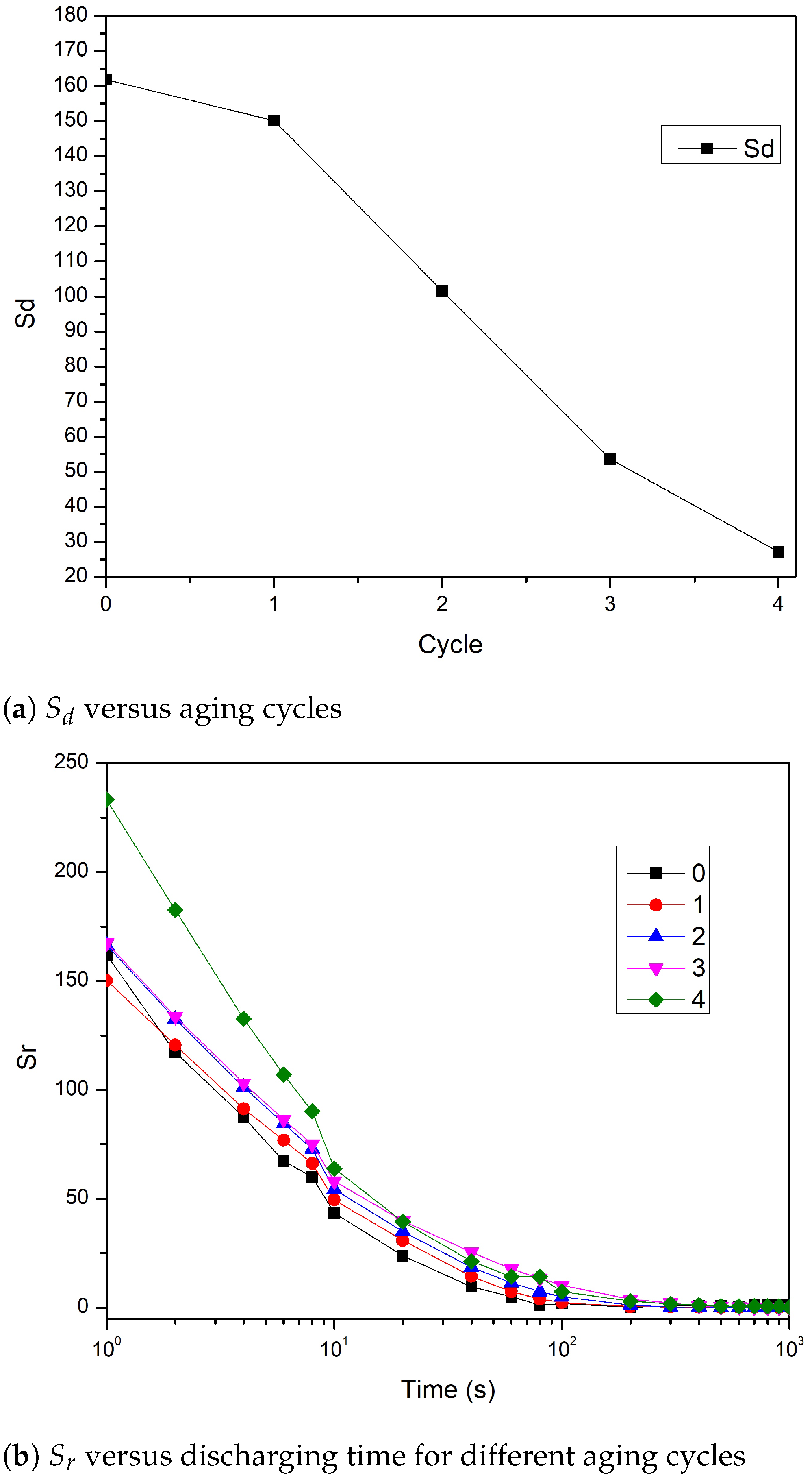
3.1.2. Results of EVR Measurement

The results of the EVR measurement for the SZRMtKVM-type cable is shown in Figure 8. Figure 8a illustrates the changes in $S_d$ with aging. A clear increase was observed in the first two aging rounds for $S_d$. A slight reduction was observed in the third round. Nevertheless, the overall $S_d$ increased from 2.248 V/s to 26.109 V/s over the course of three aging rounds.

As discussed in the previous section, the total discharging period has been divided into smaller discharging points for the EVR measurement. $S_r$ has been measured after each of these discharging points. Figure 8b depicts the changes in $S_r$ in relation to the discharging times, presented in a semilog chart. A minor decrease was observed after the first aging round in the initial discharging points. The subsequent two aging rounds showed an increasing trend compared to the unaged result.

3.1.3. Shore D Hardness

The Shore D hardness measurement was introduced in the previous section. At least ten random measuring points were selected for more accuracy, and the measurement was performed. The average of these ten measurements was then calculated. A slight increase in the Shore D readings was observed at the end of eighteen hours of thermal aging, with the hardness of the jacket increasing from 44.02 to 46.08, as shown in Figure 9.

3.2. NYCWY-Type Cable

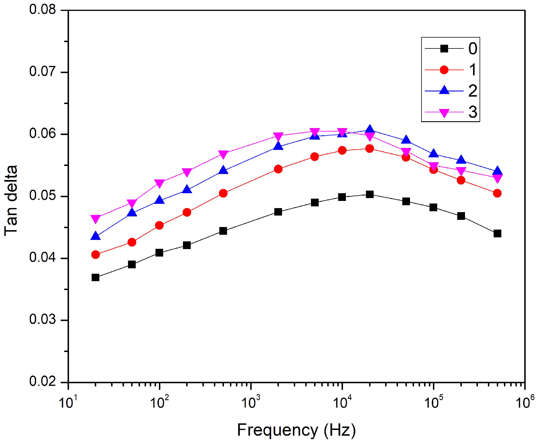
3.2.1. Results of Tan $\delta$ Measurement

The tan $\delta$ values were registered and presented in a log chart in a frequency range from 20 Hz to 500 kHz in Figure 10. The logarithmic steps were considered for determining the target frequencies. The curve’s characteristic for the NYCWY sample differed slightly from that of its SZRMtKVM counterpart. The typical pattern of the tan $\delta$ curve can be described as follows: The loss factor initially decreased with the frequency increase from 20 Hz to 50 Hz, then rose until it reached its peak value. After reaching this peak, it started to decline as the frequency increased. The most significant increase was observed in the first aging round, where tan $\delta$ rose at every frequency compared to the unaged condition (0 cycles). The loss factor continued to increase until 500 Hz in the second aging round compared to the first one, with no significant difference observed for frequencies above 500 Hz. The third and fourth rounds exhibited a noticeable increase until they reached their respective peak values, from which tan $\delta$ reduced with the increase in frequency. However, a shift in the peak values of the curves was clearly observed from the initial 200 kHz to 20 kHz.

3.2.2. Results of EVR Measurement

The results of the EVR measurement for the NYCWY-type cable are shown in Figure 11. Figure 11a illustrates the changes in $S_d$ with aging. It seemed to have a decreasing trend with the increase of aging rounds. $S_d$ dropped to 27.129 V/s from 161.86 V/s at the end of the fourth aging cycle.

Figure 11b illustrates the changes in $Sr$ against the discharging times, shown in a semilog chart. A clear increasing trend, particularly in the fourth cycle, was observed.

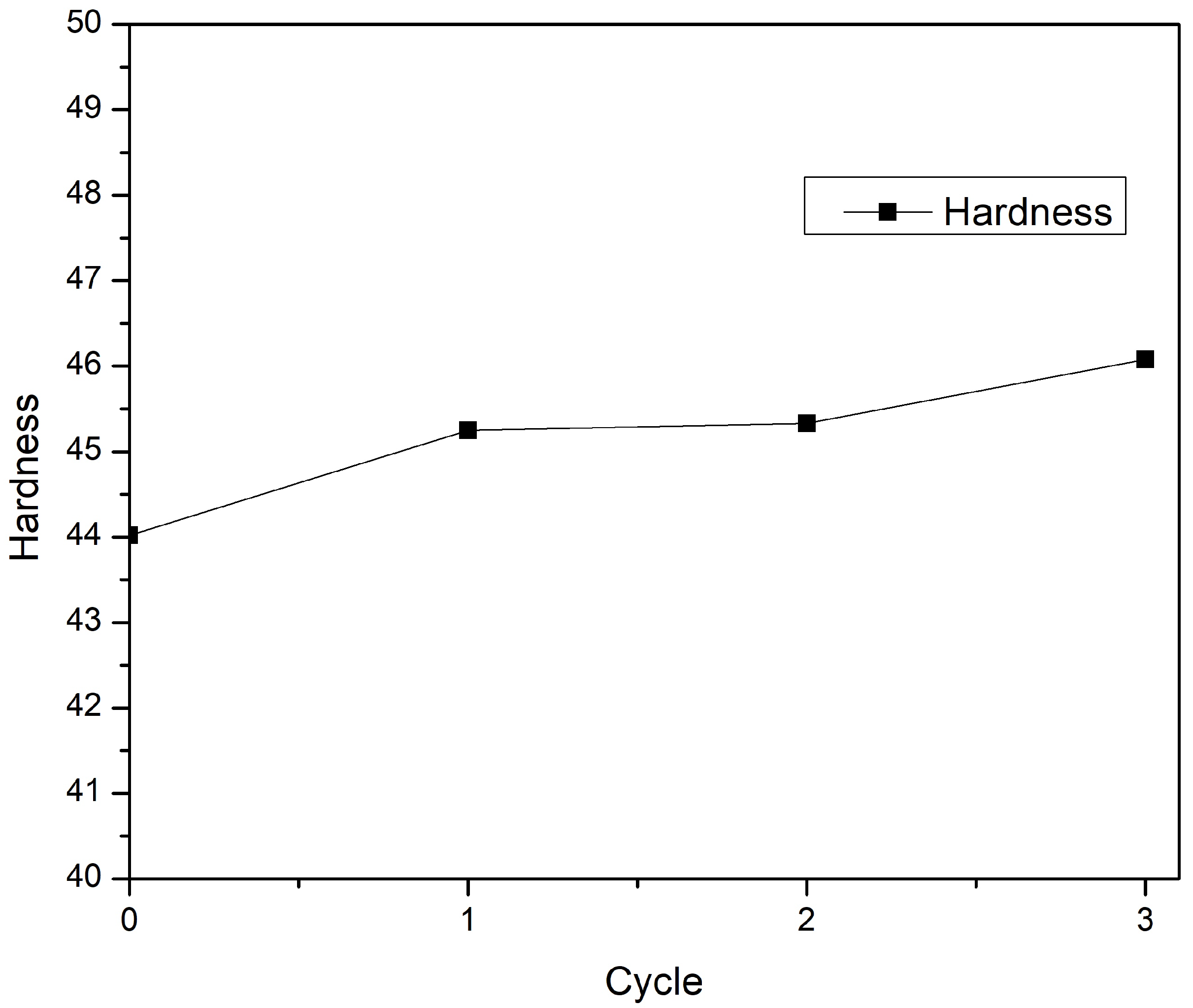
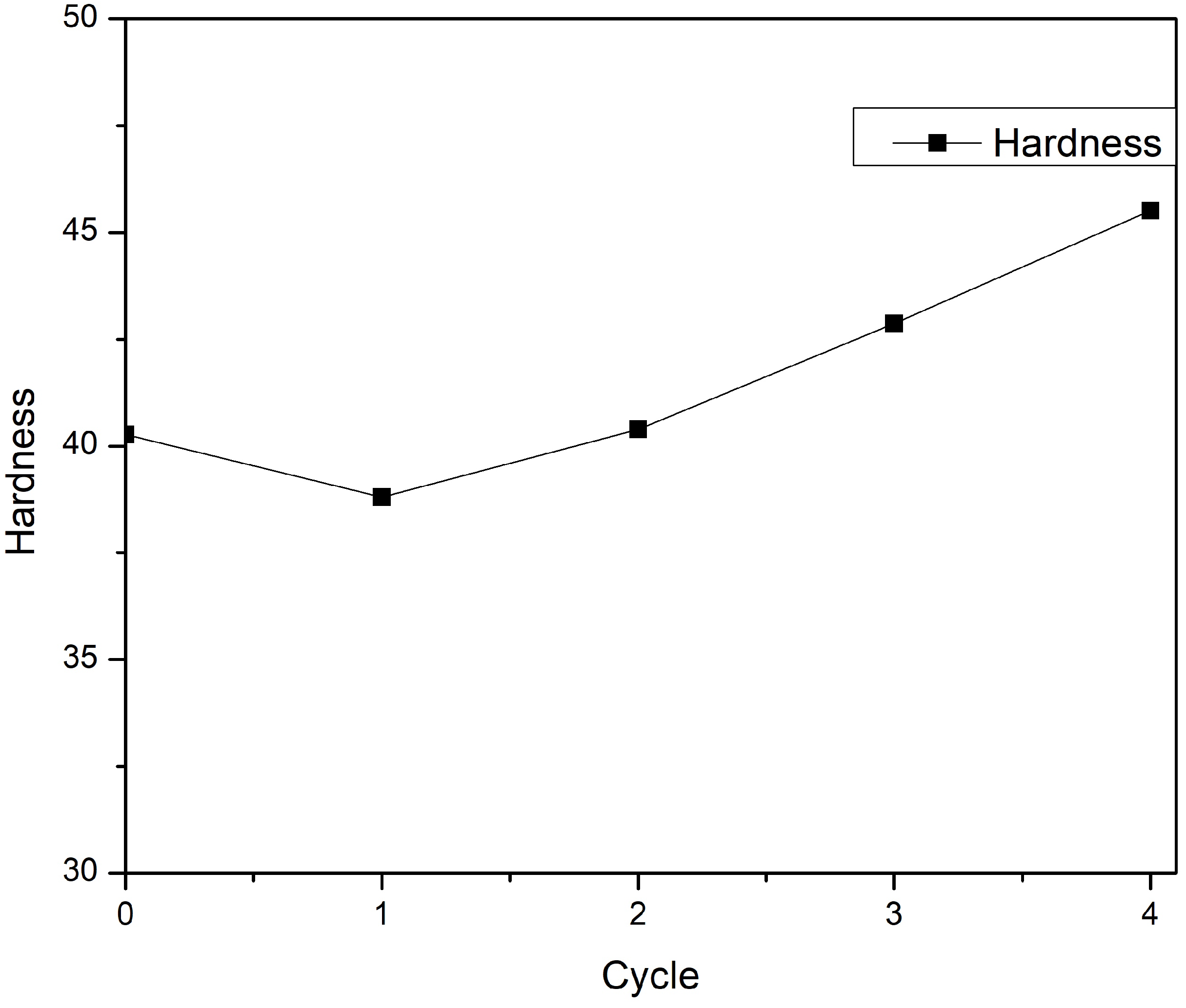
3.2.3. Shore D Hardness

The Shore D hardness measurement was performed in the previous section. At least ten random measuring points were selected for more accuracy, and the measurement was performed. The average of these ten measurements was then calculated. An initial decrease in the hardness measurement was observed, indicating slight softening on the jacket. Further aging rounds showed a monotonic increase, as shown in Figure 12. Overall, the Shore D value increased from 40.27 to 45.52.

4. Discussion

Our research has employed different measurement techniques to explore aging phenomena in different LV PVC-insulated cables. This discussion will focus on comparing these findings, identifying correlations and assessing their implications for the broader field of study.

4.1. Tan $\delta$ Measurement

It is known that, in a normal air atmosphere, three degradation mechanisms play a role in PVC and affect its dielectric properties. These are dehydrochlorination, oxidation, and the migration of plasticizers [53]. Thermal stress can cause morphological alterations within the polymer chain, potentially leading to the formation of dipolar products. These products can induce electric dipole rotation, resulting in an increase in polarization losses.

Five frequency points were chosen to simplify the analysis. These points included the following:

• 50 Hz.
• 100 Hz.
• 2 kHz.
• 5 kHz.
• 500 kHz.

Figure 13 depicts the changes in tan $\delta$ for the chosen frequencies: 50 Hz, 100 Hz, 2 kHz, 5 kHz, and 500 kHz. It is possible to observe that the tan $\delta$ increase was more dominant in every aging cycle for the low frequencies of 50 Hz and 100 Hz. The rise in the tan $\delta$ values may be linked to the presence of radicals, which contribute to both interfacial and dipolar polarization losses in the low-frequency range [36].

It is observed that the gradient of the lines is becoming smaller, and the curves are becoming flatter at higher frequencies with an increased aging cycle. High thermal stress could potentially lead to a decrease in the quantity of small molecules. Consequently, these molecules may exhibit a diminished response to a rapidly changing electric field. This could impose limitations on the increase of tan $\delta$ and, in certain instances, result in a reduction [54].

4.2. EVR Measurement

The decay voltage slope ($S_d$) results are depicted in Figure 8a for SZRMtKVM and Figure 11a for NYCWY, respectively. $S_d$ exhibited contrasting behaviors for these samples. It demonstrated an increasing trend with aging in the case of SZRMtKVM, whereas it showed a decreasing trend with aging for NYCWY. As previously mentioned, $S_d$ is proportional to specific conductivity. Therefore, an elevation in $S_d$ might be attributed to increased specific conductivity.

For the case of return voltage slope $S_r$, the chart that shows $S_r$ at a 1 s discharging time is shown to visualize the trend better. Therefore, $S_r$ at a 1 s discharging time is presented in Figure 14. The results of $S_r$ showed a small, but clear increasing trend for SZRMtKVM. However, a more surprising result can be seen in the case of NYCWY with the sudden jump in the fourth aging round from the value of 161.806 V/s to 233.09 V/s. This jump might be due to the increase in the interfacial polarization.

Table 1. Ratio of $S_r$ at 1 s discharging time before and after aging.

	SZRMtKVM	NYCWY
Before	61.856	161.806
After	70.369	233.09
Ratio (After/Before)	1.13	1.44

presents the calculated ratios of $S_r$ at 1 s discharging time values before and after aging.

4.3. Shore D Hardness

Figure 9 and Figure 12 depict the result of the hardness measurement. It commonly understood that the dominant degradation process for plasticized PVC is plasticizer loss at this aging temperature [37,53]. The SZRMtKVM sample exhibited a gradual increase in hardness. In contrast, the hardness of the NYCWY sample initially decreased after the first aging cycle, but then, started to increase at a higher rate. The initial reduction in hardness could be attributed to the annealing effect. It is possible that the annealing effect may mask the plasticizer loss in the first round [37,38,55,56]. After that, the plasticizer loss became dominant as the material’s hardness increased [39]. Nedjar et al. presented similar observations in their research by using different mechanical measurements such as Elongation at Break (EaB) and tensile strength. The authors first observed a reduction in tensile strength in the initial cycles before it started to increase [57].

Table 2. Ratio of Shore D hardness of samples before and after aging.

	SZRMtKVM	NYCWY
Before	44.02	40.27
After	46.08	45.52
Ratio (After/Before)	1.046	1.13

presents the calculated ratios of the Shore D values before and after aging.

4.4. Correlation between Electrical and Mechanical Quantities

The detailed analysis of short-term cyclic thermal aging in each cable type individually has been published elsewhere [38,46,48]. Additionally, similar findings can be observed in another independent study conducted by a different laboratory, which utilized similar techniques such as tan $\delta$, Shore D, and EVR. However, $S_r$ was not investigated in that study [39].

To identify a suitable condition-monitoring technique and aging marker for these two cable types, the coefficient of determination ($R^2$) was calculated between the electrical quantities and Shore D hardness values. The calculated $R^2$ values can be seen in

Table 3. Correlation values between Shore D hardness and different electrical quantities for both cable types.

Electrical Quantity		${\mathit{R}}^2$
		SZRMtKVM	NYCWY
50 Hz	tan $\delta$	0.8493	0.5866
100 Hz	tan $\delta$	0.908	0.5974
2 kHz	tan $\delta$	0.9317	0.3648
5 kHz	tan $\delta$	0.9059	0.2488
500 kHz	tan $\delta$	0.8025	0.5374
$S_d$	EVR	0.7548	0.8367
$S_r$ 1 s	EVR	0.8875	0.8289

.

The tan $\delta$ results at certain frequencies, $S_d$, and $S_r$ were applied for a correlation analysis with the Shore D results. $S_r$ at 1 s exhibited a strong correlation with hardness for both types of cables, with $R^2$ values of 0.8875 for SZRMtKVM and 0.8289 for NYCWY. Additionally, tan $\delta$ at the 50 Hz, 100 Hz, and 2 kHz frequencies showed a good correlation with the highest $R^2$ value of 0.9317 for the SZRMtKVM cable, while frequency domain spectroscopy demonstrated a weak correlation with the highest value of 0.5974 for NYCWY.

The following outcomes can be obtained from the analysis:

• For SZRMtKVM type:

  -

  The highest correlation between the mechanical and electrical measurements was observed at a frequency of 2 kHz. Therefore, it can be concluded that 2 kHz can be utilized as an aging marker for the FDS technique.

  -

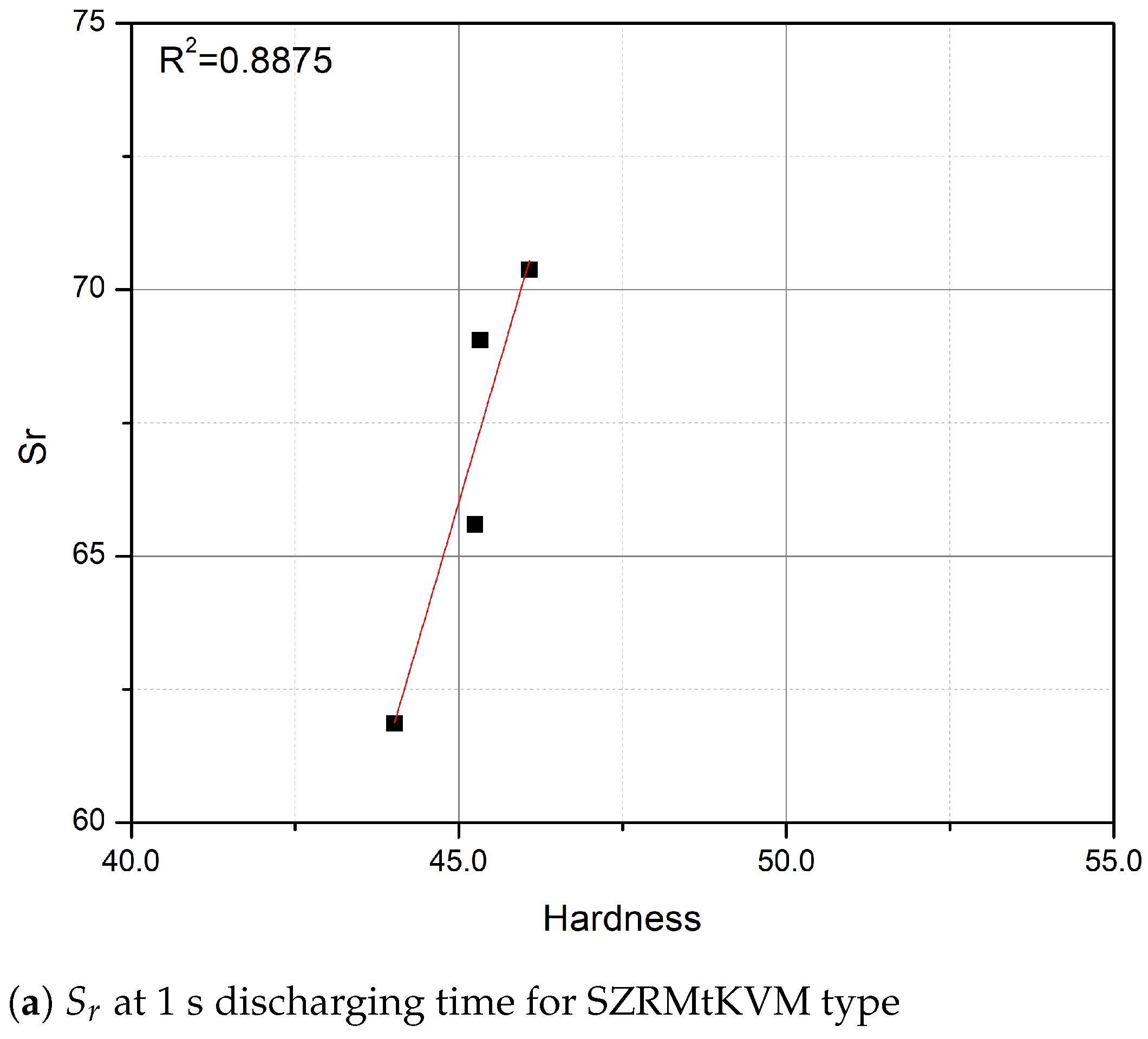
  The $S_r$ measurement at a 1-s discharging time exhibited a strong correlation with the hardness measurement. Therefore, it can also be utilized as an aging marker in the TDS technique.

  -

  Overall, in the case of SZRMtKVM, the FDS technique demonstrated a slightly better correlation with aging compared to the TDS technique at frequency points of 100 Hz, 2 kHz, and 5 kHz.

• For NYCWY type:

  -

  The frequency domain spectroscopy (FDS) technique exhibited a weak correlation with hardness, with the highest coefficient of determination ($R^2$) of 0.5974 observed at a frequency of 100 Hz.

  -

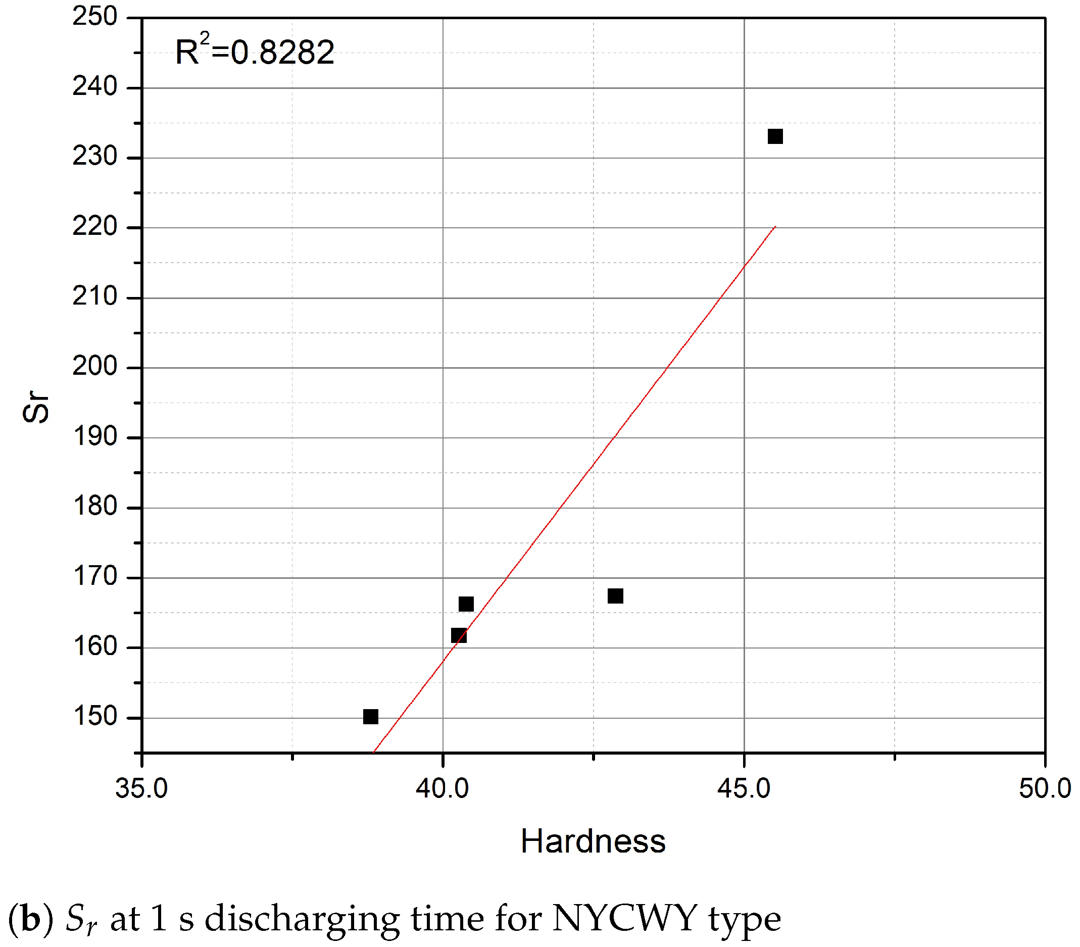
  The time domain spectroscopy (TDS) technique demonstrated a relatively strong correlation, with coefficient of determination ($R^2$) values above 0.8 for both $Sr$ and $Sd$.

The cross-comparison of the results indicated that $S_r$ at a 1 s discharging time can be utilized as an electrical aging marker as it gave acceptable results for both cable types. This marker is plotted in Figure 15.

5. Conclusions

This paper investigates the overall degradation of two PVC-insulated LV distribution cables exposed to short-term cyclic aging. The effect of short-term thermal aging was investigated by two non-destructive CM techniques: tan $\delta$ and EVR. Furthermore, the hardness of the jacket was measured by a Shore D hardness tester. The results obtained by the measurements were used for the correlation analysis between the electrical quantifiers and Shore D results.

This analysis clearly demonstrated a strong correlation between the tan $\delta$ values at various frequencies and the Shore D hardness for the SZRMtKVM type, unlike the NYCWY type. While the R-squared values—0.8875 for SZRMtKVM and 0.8289 for NYCWY—may not represent the absolute highest, they still indicated a significant correlation for both cables concerning the slope of the return voltage after 1 s of discharging time. Therefore, the slope of the return voltage was conclusively established as a dependable condition-monitoring indicator for these types of cables.

The results presented in this paper serve as a solid foundation for finding common condition-monitoring systems for different types of cables in the grid. The future work for this research involves increasing the number of data points for the correlation analysis. This would require conducting additional aging cycles to validate the findings. One typical limitation of this study is the use of brand-new, unaged cables for laboratory aging experiments. The findings can be enhanced by extending this research to include service-aged cables that have been removed from the grid.

References

- Mohajan, H. Greenhouse gas emissions increase global warming. Int. J. Econ. Political Integr. 2011, 1, 21–34. [Google Scholar]
- Lashof, D.A.; Ahuja, D.R. Relative contributions of greenhouse gas emissions to global warming. Nature 1990, 344, 529–531. [Google Scholar] [CrossRef]
- Holechek, J.L.; Geli, H.M.E.; Sawalhah, M.N.; Valdez, R. A Global Assessment: Can Renewable Energy Replace Fossil Fuels by 2050? Sustainability 2022, 14, 4792. [Google Scholar] [CrossRef]
- Chen, B.; Xiong, R.; Li, H.; Sun, Q.; Yang, J. Pathways for sustainable energy transition. J. Clean. Prod. 2019, 228, 1564–1571. [Google Scholar] [CrossRef]
- Bouffard, F.; Kirschen, D.S. Centralised and distributed electricity systems. Energy Policy 2008, 36, 4504–4508. [Google Scholar] [CrossRef]
- Mehigan, L.; Deane, J.; Gallachóir, B.; Bertsch, V. A review of the role of distributed generation (DG) in future electricity systems. Energy 2018, 163, 822–836. [Google Scholar] [CrossRef]
- Worighi, I.; Maach, A.; Hafid, A.; Hegazy, O.; Van Mierlo, J. Integrating renewable energy in smart grid system: Architecture, virtualization and analysis. Sustain. Energy Grids Netw. 2019, 18, 100226. [Google Scholar] [CrossRef]
- Istók, R.; Kádár, P. Active and reactive power of solar electric vehicle chargers system. Pollack Period. 2023, 18, 95–100. [Google Scholar] [CrossRef]
- Ourahou, M.; Ayrir, W.; EL Hassouni, B.; Haddi, A. Review on smart grid control and reliability in presence of renewable energies: Challenges and prospects. Math. Comput. Simul. 2020, 167, 19–31. [Google Scholar] [CrossRef]
- Wang, J.; Zhou, N.; Ran, Y.; Wang, Q. Optimal Operation of Active Distribution Network Involving the Unbalance and Harmonic Compensation of Converter. IEEE Trans. Smart Grid 2019, 10, 5360–5373. [Google Scholar] [CrossRef]
- Atrigna, M.; Buonanno, A.; Carli, R.; Cavone, G.; Scarabaggio, P.; Valenti, M.; Graditi, G.; Dotoli, M. A Machine Learning Approach to Fault Prediction of Power Distribution Grids under Heatwaves. IEEE Trans. Ind. Appl. 2023, 59, 4835–4845. [Google Scholar] [CrossRef]
- Pompili, M.; Calcara, L.; D’Orazio, L.; Ricci, D.; Derviškadić, A.; He, H. Joints defectiveness of MV underground cable and the effects on the distribution system. Electr. Power Syst. Res. 2021, 192, 107004. [Google Scholar] [CrossRef]
- Iweh, C.D.; Gyamfi, S.; Tanyi, E.; Effah-Donyina, E. Distributed Generation and Renewable Energy Integration into the Grid: Prerequisites, Push Factors, Practical Options, Issues and Merits. Energies 2021, 14, 5375. [Google Scholar] [CrossRef]
- Celina, M.; Gillen, K.; Assink, R. Accelerated aging and lifetime prediction: Review of non-Arrhenius behaviour due to two competing processes. Polym. Degrad. Stab. 2005, 90, 395–404. [Google Scholar] [CrossRef]
- Celina, M.C. Review of polymer oxidation and its relationship with materials performance and lifetime prediction. Polym. Degrad. Stab. 2013, 98, 2419–2429. [Google Scholar] [CrossRef]
- Zhou, C.; Yi, H.; Dong, X. Review of recent research towards power cable life cycle management. High Volt. 2017, 2, 179–187. [Google Scholar] [CrossRef]
- Choudhary, M.; Shafiq, M.; Kiitam, I.; Hussain, A.; Palu, I.; Taklaja, P. A Review of Aging Models for Electrical Insulation in Power Cables. Energies 2022, 15, 3408. [Google Scholar] [CrossRef]
- Densley, J. Ageing mechanisms and diagnostics for power cables—An overview. IEEE Electr. Insul. Mag. 2001, 17, 14–22. [Google Scholar] [CrossRef]
- Hancox, N.L. Thermal effects on polymer matrix composites: Part 1. Thermal cycling. Mater. Des. 1998, 19, 85–91. [Google Scholar] [CrossRef]
- Jakubowicz, I.; Yarahmadi, N.; Gevert, T. Effects of accelerated and natural ageing on plasticized polyvinyl chloride (PVC). Polym. Degrad. Stab. 1999, 66, 415–421. [Google Scholar] [CrossRef]
- Quennehen, P.; Royaud, I.; Seytre, G.; Gain, O.; Rain, P.; Espilit, T.; François, S. Determination of the aging mechanism of single core cables with PVC insulation. Polym. Degrad. Stab. 2015, 119, 96–104. [Google Scholar] [CrossRef]
- Ekelund, M.; Edin, H.; Gedde, U. Long-term performance of poly(vinyl chloride) cables. Part 1: Mechanical and electrical performances. Polym. Degrad. Stab. 2007, 92, 617–629. [Google Scholar] [CrossRef]
- Wilson, A.S. Plasticisers: Selection, Applications and Implications; iSmithers Rapra Publishing: Shrewsbury, UK, 1996; Volume 88. [Google Scholar]
- Gumargalieva, K.; Ivanov, V.; Zaikov, G.; Moiseev, J.V.; Pokholok, T. Problems of ageing and stabilization of poly (vinyl chloride). Polym. Degrad. Stab. 1996, 52, 73–79. [Google Scholar] [CrossRef]
- You, S.; Segerberg, H. Integration of 100% micro-distributed energy resources in the low voltage distribution network: A Danish case study. Appl. Therm. Eng. 2014, 71, 797–808. [Google Scholar] [CrossRef]
- Muniz, P.R.; Teixeira, J.L.; Santos, N.Q.; Magioni, P.L.Q.; Cani, S.P.N.; Fardin, J.F. Prospects of life estimation of low voltage electrical cables insulated by PVC by emissivity measurement. IEEE Trans. Dielectr. Electr. Insul. 2017, 24, 3951–3958. [Google Scholar] [CrossRef]
- Babrauskas, V. Mechanisms and modes for ignition of low-voltage PVC wires, cables, and cords. In Proceedings of the Fire and Materials Conference, San Francisco, CA, USA, 31 January–1 February 2005; pp. 291–309. [Google Scholar]
- Kruizinga, B.; Wouters, P.; Steennis, E. Comparison of polymeric insulation materials on failure development in low-voltage underground power cables. In Proceedings of the 2016 IEEE Electrical Insulation Conference (EIC), Montreal, QC, Canada, 19–22 June 2016; IEEE: Piscataway, NJ, USA, 2016; pp. 444–447. [Google Scholar]
- Buhari, M.; Levi, V.; Kapetanaki, A. Cable Replacement Considering Optimal Wind Integration and Network Reconfiguration. IEEE Trans. Smart Grid 2018, 9, 5752–5763. [Google Scholar] [CrossRef]
- Kruizinga, B.; Wouters, P.A.A.F.; Steennis, E.F. Fault development upon water ingress in damaged low voltage underground power cables with polymer insulation. IEEE Trans. Dielectr. Electr. Insul. 2017, 24, 808–816. [Google Scholar] [CrossRef]
- Ringsberg, J.W.; Dieng, L.; Li, Z.; Hagman, I. Characterization of the Mechanical Properties of Low Stiffness Marine Power Cables through Tension, Bending, Torsion, and Fatigue Testing. J. Mar. Sci. Eng. 2023, 11, 1791. [Google Scholar] [CrossRef]
- Verardi, L.; Fabiani, D.; Montanari, G.C. Electrical aging markers for EPR-based low-voltage cable insulation wiring of nuclear power plants. Radiat. Phys. Chem. 2014, 94, 166–170. [Google Scholar] [CrossRef]
- Bowler, N.; Liu, S. Aging mechanisms and monitoring of cable polymers. Int. J. Progn. Health Manag. 2015, 6. [Google Scholar] [CrossRef]
- Sriraman, A.; Bowler, N.; Glass, S.; Fifield, L.S. Dielectric and Mechanical Behavior of Thermally Aged EPR/CPE Cable Materials. In Proceedings of the 2018 IEEE Conference on Electrical Insulation and Dielectric Phenomena (CEIDP), Cancun, Mexico, 21–24 October 2018; pp. 598–601. [Google Scholar] [CrossRef]
- Fabiani, D.; Suraci, S.V. Broadband Dielectric Spectroscopy: A Viable Technique for Aging Assessment of Low-Voltage Cable Insulation Used in Nuclear Power Plants. Polymers 2021, 13, 494. [Google Scholar] [CrossRef] [PubMed]
- Mustafa, E.; Afia, R.S.; Tamus, Z.Á. Dielectric loss and extended voltage response measurements for low-voltage power cables used in nuclear power plant: Potential methods for aging detection due to thermal stress. Electr. Eng. 2021, 103, 899–908. [Google Scholar] [CrossRef]
- Bal, S.; Tamus, Z.A. Investigation of the Structural Dependence of the Cyclical Thermal Aging of Low-Voltage PVC-Insulated Cables. Symmetry 2023, 15, 1186. [Google Scholar] [CrossRef]
- Csányi, G.M.; Bal, S.; Tamus, Z.A. Dielectric Measurement Based Deducted Quantities to Track Repetitive, Short-Term Thermal Aging of Polyvinyl Chloride (PVC) Cable Insulation. Polymers 2020, 12, 2809. [Google Scholar] [CrossRef] [PubMed]
- Paun, C.; Gavrila, D.E.; Paltanea, V.M.; Stoica, V.; Paltanea, G.; Nemoianu, I.V.; Ionescu, O.; Pistritu, F. Study on the Behavior of Low-Voltage Cable Insulation Subjected to Thermal Cycle Treatment. Sci. Bull. Electr. Eng. Fac. 2023, 23, 34–39. [Google Scholar] [CrossRef]
- IEC 60502-1; Power Cables with Extruded Insulation and Their Accessories for Rated Voltages from 1 kV (Um = 1.2 kV) Up to 30 kV (Um = 36 kV)—Part 1: Cables for Rated Voltages of 1 kV (Um = 1.2 kV) and 3 kV (Um = 3.6 kV). International Electrotechnical Commision (IEC): Geneva, Switzerland, 2004.
- Zaengl, W. Dielectric spectroscopy in time and frequency domain for HV power equipment. I. Theoretical considerations. IEEE Electr. Insul. Mag. 2003, 19, 5–19. [Google Scholar] [CrossRef]
- Bal, S.; Tamus, Z.A. Investigation of Effects of Thermal Ageing on Dielectric Properties of Low Voltage Cable Samples by using Dielectric Response Analyzer. In Proceedings of the 2022 International Conference on Diagnostics in Electrical Engineering (Diagnostika), Pilsen, Czech Republic, 6–8 September 2022; pp. 1–6. [Google Scholar] [CrossRef]
- Fofana, I.; Hadjadj, Y. Electrical-Based Diagnostic Techniques for Assessing Insulation Condition in Aged Transformers. Energies 2016, 9, 679. [Google Scholar] [CrossRef]
- Zhang, T.; Mandala, A.T.; Zhong, T.; Zhang, N.; Jiang, S. Identification of extended Debye model parameters for oil-paper insulation based on voltage response characteristic. Electr. Eng. 2022, 104, 2379–2387. [Google Scholar] [CrossRef]
- Mustafa, E.; Afia, R.S.; Tamus, Z.Á. Condition assessment of low voltage photovoltaic DC cables under thermal stress using non-destructive electrical techniques. Trans. Electr. Electron. Mater. 2020, 21, 503–512. [Google Scholar] [CrossRef]
- Bal, S.; Tamus, Z.A. Investigation of Effects of Short-term Thermal Stress on PVC Insulated Low Voltage Distribution Cables. Period. Polytech. Electr. Eng. Comput. Sci. 2021, 65, 167–173. [Google Scholar] [CrossRef]
- Tamus, Z.; Berta, I. Application of voltage response measurement on low voltage cables. In Proceedings of the 2009 IEEE Electrical Insulation Conference, Montreal, QC, Canada, 31 May 2009–3 June 2009; IEEE: Piscataway, NJ, USA, 2009; pp. 444–447. [Google Scholar]
- Bal, S.; Tamus, Z.A. Analyzing the Effect of Thermal Stress on Dielectric Parameters of PVC Insulated Low Voltage Cable Sample. In Proceedings of the 2022 IEEE 5th International Conference and Workshop Óbuda on Electrical and Power Engineering (CANDO-EPE), Budapest, Hungary, 21–22 November 2022; IEEE: Piscataway, NJ, USA, 2022; pp. 000067–000072. [Google Scholar]
- ASTM D2240-05; Standard Test Method for Rubber Property: Durometer Hardness. ASTM West Conshohocken: Conshohocken, PA, USA, 2010.
- Chatterjee, S.; Hadi, A.S. Regression Analysis by Example; John Wiley & Sons: Hoboken, NJ, USA, 2013. [Google Scholar]
- Gogtay, N.; Deshpande, S.; Thatte, U. Principles of regression analysis. J. Assoc. Physicians India 2017, 65, 48–52. [Google Scholar] [PubMed]
- Tamus, Z.Á. Regression analysis to evaluate the reliability of insulation diagnostic methods. J. Electrost. 2013, 71, 564–567. [Google Scholar] [CrossRef]
- Linde, E.; Gedde, U.W. Plasticizer migration from PVC cable insulation–The challenges of extrapolation methods. Polym. Degrad. Stab. 2014, 101, 24–31. [Google Scholar] [CrossRef]
- He, D.; Gu, J.; Wang, W.; Liu, S.; Song, S.; Yi, D. Research on mechanical and dielectric properties of XLPE cable under accelerated electrical-thermal aging. Polym. Adv. Technol. 2017, 28, 1020–1029. [Google Scholar] [CrossRef]
- Ito, M.; Nagai, K. Analysis of degradation mechanism of plasticized PVC under artificial aging conditions. Polym. Degrad. Stab. 2007, 92, 260–270. [Google Scholar] [CrossRef]
- Audouin, L.; Dalle, B.; Metzger, G.; Verdu, J. Thermal aging of plasticized PVC. II. Effect of plasticizer loss on electrical and mechanical properties. J. Appl. Polym. Sci. 1992, 45, 2097–2103. [Google Scholar] [CrossRef]
- Nedjar, M.; Boubakeur, A.; Beroual, A.; Bournane, M. Thermal aging of polyvinyl chloride used in electrical insulation. In Annales de Chimie Science des Matériaux; Elsevier: Amsterdam, The Netherlands, 2003; Volume 28, pp. 97–104. [Google Scholar]