Article

Noncontact Automatic Water-Level Assessment and Prediction in an Urban Water Stream Channel of a Volcanic Island Using Deep Learning

by
Fábio Mendonça
1,2,*,
Sheikh Shanawaz Mostafa
2,
Fernando Morgado-Dias
1,2,
Joaquim Amândio Azevedo
1,
Antonio G. Ravelo-García
2,3 and
Juan L. Navarro-Mesa
3
1
Faculty of Exact Sciences and Engineering, University of Madeira, 9020-105 Funchal, Portugal
2
Interactive Technologies Institute (ITI/LARSyS) and ARDITI, 9020-105 Funchal, Portugal
3
Institute for Technological Development and Innovation in Communications, Universidad de Las Palmas de Gran Canaria, 35017 Las Palmas de Gran Canaria, Spain
*
Author to whom correspondence should be addressed.
Electronics 2024, 13(6), 1145; https://doi.org/10.3390/electronics13061145
Submission received: 23 February 2024 / Revised: 15 March 2024 / Accepted: 19 March 2024 / Published: 20 March 2024
(This article belongs to the Special Issue Selected Papers from Young Researchers in AI for Computer Vision)

Abstract

:
Traditional methods for water-level measurement usually employ permanent structures, such as a scale built into the water system, which is costly and laborious and can wash away with water. This research proposes a low-cost, automatic water-level estimator that can appraise the level without disturbing water flow or affecting the environment. The estimator was developed for urban areas of a volcanic island water channel, using machine learning to evaluate images captured by a low-cost remote monitoring system. For this purpose, images from over one year were collected. For better performance, captured images were processed by converting them to a proposed color space, named HLE, composed of hue, lightness, and edge. Multiple residual neural network architectures were examined. The best-performing model was ResNeXt, which achieved a mean absolute error of 1.14 cm using squeeze and excitation and data augmentation. An explainability analysis was carried out for transparency and a visual explanation. In addition, models were developed to predict water levels. Three models successfully forecasted the subsequent water levels for 10, 60, and 120 min, with mean absolute errors of 1.76 cm, 2.09 cm, and 2.34 cm, respectively. The models could follow slow and fast transitions, leading to a potential flooding risk-assessment mechanism.

1. Introduction

As urban development and expansion progress, so does the need for new land to accommodate the urban expansion, leading the infrastructures to appear in locations where natural hazards can occur [1]. Such threats include flash floods, where low-lying areas experience rapid flooding. These usually occur during high-intensity rainfall and provide little warning time to the population. Thus, these events are considered one of the main challenges for regional water security, especially for rural settlements in mountainous areas, since gravitational energy is provided to the water flow by steep slopes, potentially leading to substantial channel overflow downstream [2]. Prime examples of such locations are volcanic islands, where the rugged relief is associated with steep water channels that are frequently narrow and deep. Furthermore, these channels can carry substantial amounts of organic matter and sediment, increasing the downstream flooding risk [3].
Water flow monitoring is essential in numerous applications where the functional area ranges from small water streams to large rivers. The most common techniques include the use of contact-based sensors, including pressure or floating sensors, and contactless sensors, such as ultrasonic water meters and image-based methods [4]. The first approach is particularly problematic when the water current is intense, as it can damage or carry away the sensors. Furthermore, these sensors usually require calibrations to be performed frequently to maintain the measurement’s accuracy [5].
Regarding the contactless methods, although ultrasonic sensors are easy to install, they have been shown to be problematic when examining turbulent water [6], which usually happens during flooding events in volcanic islands’ water channels [3]. As a result, image-based sensors were found to be suitable for monitoring the water channels in these locations, presenting a low installation and maintenance cost [7]. However, satellite images lack enough spatial and temporal resolutions, particularly for narrow water streams [8], while the use of unmanned vehicles is likely not to be suitable for small urban areas [9]. Furthermore, an expert is needed to steer the vehicle, increasing usage costs. Hence, a fixed-location camera is likely the best solution for continuous water-level assessments based on image analysis [7].
Developing a hand-tailored system that can accommodate all characteristics of the water channel is labor-intensive and prone to environmental changes [7]. Hence, there is a need for an algorithm based on a machine learning approach that leads to models that learn the patterns directly from the data. Although the machine learning approaches previously presented have a relevant performance, they are likely unsuitable for monitoring the water levels in volcanic islands’ water channels in urban areas. In these channels, vegetation is commonly present and continuously changes, continuously growing until the next large water volume removes it, making the segmentation-based approach unfeasible. As a result, there is a need for an algorithm that forecasts the water level directly from the images, training the model on multiple conditions so that it learns to ignore the vegetation and focus only on the water level. Such an algorithm can follow the approach presented by Xu et al. [10] but without using a rule in the image. This leads to an automated model that has not been previously described in the literature and comprises the main novelty of this work. For this purpose, a dataset was created for this work and made publicly available, composed of images collected (and annotated) from a water channel in Funchal, Madeira Island, Portugal.
Employing a staff gauge or a ruler as a scale captured by a camera can lead to a low estimation error. However, water ripples, traces of precipitation in the image, and debris on the water’s surface can produce misperceptions during heavy rain [7]. Furthermore, construction can be unfeasible and lead to the destruction of the environment [11]. Following this line of thought, the main goal of this work is to propose an automatic noncontract water-level measurement method suitable for volcanic islands’ water channels in urban areas without requiring a visual scale. Such a method can be used further for emitting different alarms according to the level’s assessment. For this purpose, a fixed-camera-based methodology was employed. This article comprises five sections, presenting a state-of-the-art overview in the second section, materials and methods in the third section, while the fourth section shows and discusses the results. The last section concludes the work.

2. State-of-the-Art Overview

A common practice in state-of-the-art works that follow an image-based approach uses a staff gauge to support measurements. Chen et al. [12] and Guo et al. [13] employed image-recognition algorithms to identify the characters on the staff gauge image, achieving a mean error (ME) of 0.9 cm when predicting the water level. A similar approach was used by Zhang et al. [14], employing an image analysis algorithm to examine images from an infrared camera, achieving an error of 1 cm. Furthermore, with a similar concept, an error of 1 cm was reported by Zhang et al. [15] when using a developed image-recognition algorithm to examine a staff gauge, which can be reduced to 1 mm when using a proposed tunning strategy.
A ruler was used by Hies et al. [16] to identify the water level using the Hough transform and an edge detection algorithm. Lin et al. [17] also used this transform in a similar approach, achieving an average error of 1 cm. A different method based on machine learning was proposed by Xu et al. [10] to identify the water level by examining the characters on a staff gauge, using a Convolutional Neural Network (CNN) to evaluate images in the Hue, Saturation, and Value (HSV) color space. This approach has the advantage of not relying on tailored algorithms for a specific location, using data to tune the model automatically. A CNN was also used by Pan et al. [18] to determine the water level in a rule, attaining an average error of around 1 cm. An analogous approach was used by Qiao et al. [19] with a similar performance.
A good performance was attained in the state-of-the-art method by employing a staff gauge or a ruler as a scale. Such scale limits the applicability of these methods for narrow urban water channels, especially during heavy rain [7]. Moreover, the illumination condition on these channels is usually problematic, having substantially different intensities during day and night operations. This leads several state-of-the-art works to discard images with insufficient brightness or low contrast [7]. Therefore, there is a need for methodologies that do not require such scales. These methods can rely on examining the image patterns that allow for discriminating the water region, as carried out by Ran et al. [20], achieving a Mean Squared Error (MSE) of about 4 cm. Stumpf et al. [21] also evaluated specific patterns in an installation site to determine the water level and reported a Mean Absolute Percentage Error (MAPE) of 9%.
Nevertheless, the methods that do not employ a rule commonly rely on edge detection methods. Udomsiri and Iwahashi [22] proposed an edge detection methodology to identify horizontal lines associated with water levels. A more complex approach was proposed by Ridolfi and Manciola [23] using the Canny edge detection algorithm to determine the water line and then assess the level by detecting reference points, reporting a Mean Absolute Error (MAE) of around 5 cm. A similar concept was used by Eltner et al. [24] with an error of about 2 cm. Young et al. [25] also used edge detection, but evaluated the clear edge of rocks to determine the water margin, reporting an average error of about 3 cm. Azevedo and Brás [7] used edge detection to identify a region of interest to calibrate an image and then employed a gradient-based analysis to estimate the water level in volcanic islands’ water channels.
Similar to the approaches based on a scale, the use of tailored algorithms for a specific location limits the applicability of the previously examined methods for other sites. On the other hand, using a machine learning approach leads to models that learn the patterns directly from the data, developing algorithms that are likely more resilient to environmental changes, such as [26]: calm and turbulent water flow; clear and opaque water (during floods with sediments); the presence of shadows that vary during the year; high- and low-contrast images; and clear and foggy days. Furthermore, these models can be transfer-learned to other locations, even if a retraining procedure is required. A machine learning approach with images fed to a CNN to perform water segmentation was proposed by Eltner et al. [26], comparing the assessed water contour with a reconstructed model to determine the water level, reporting an error that ranged from around 1 to 4 cm. A similar approach was also employed by Vandaele et al. [27].

3. Materials and Methods
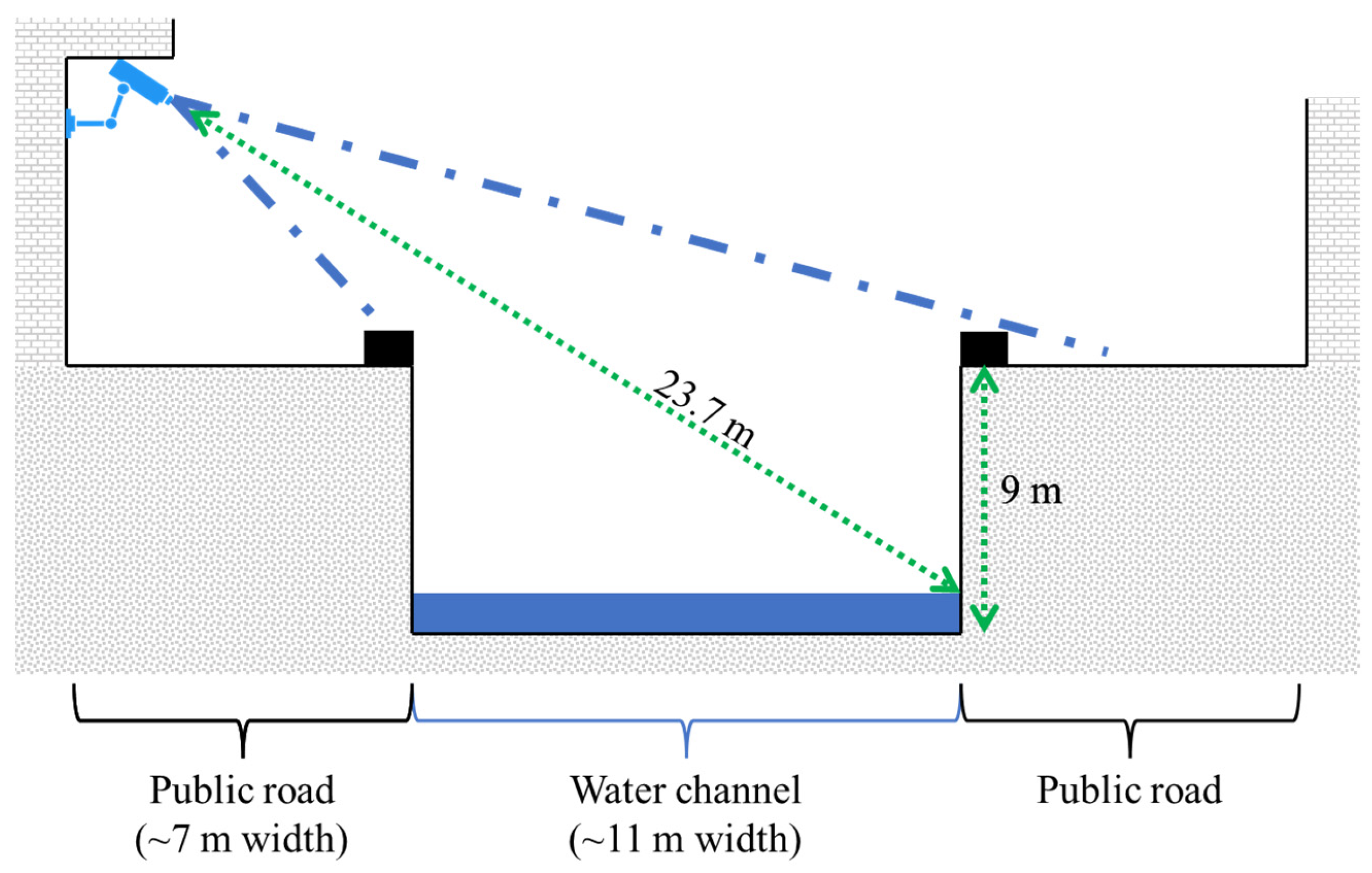
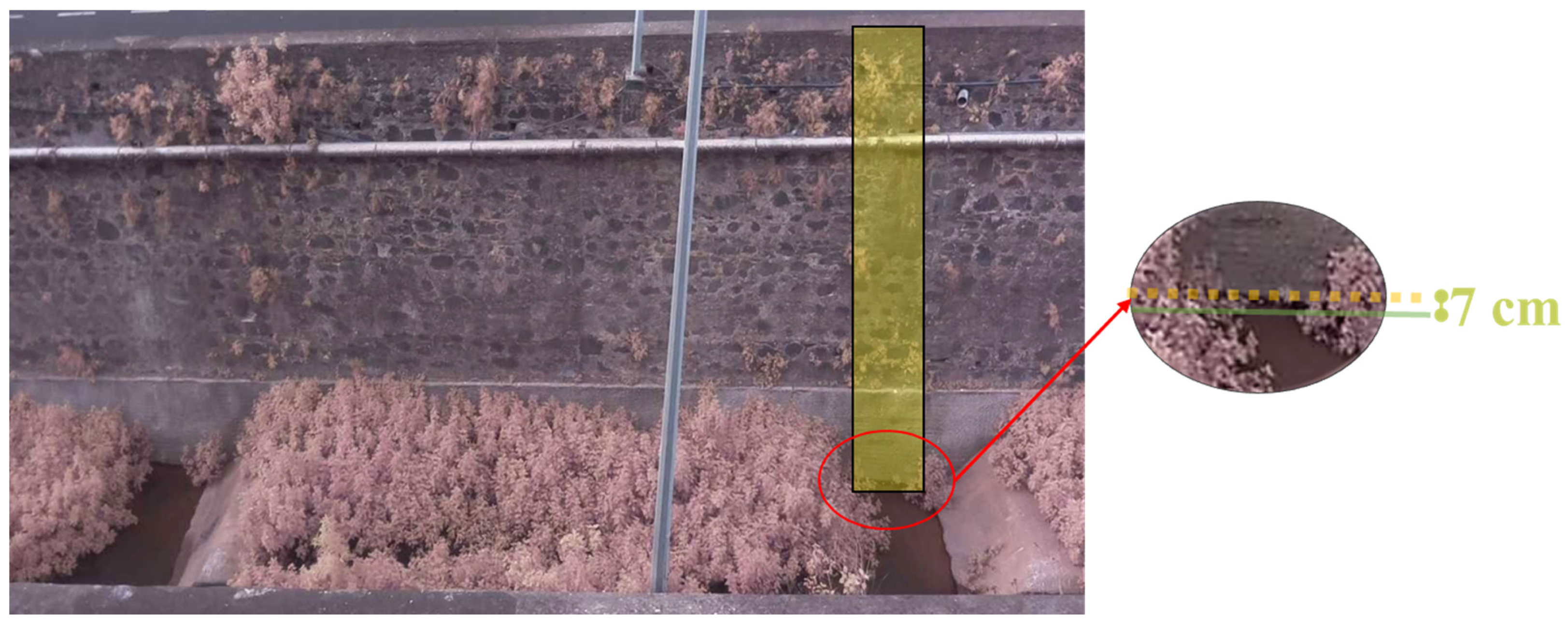
The selected location for the study was in an urban area’s water channel on a volcanic island, continuously capturing images with a low-cost commercial device. These images were then annotated regarding the water level. Following a similar approach to Xu et al.’s [10], the color space of the images was initially changed, although Hue, Saturation, and Lightness (HSL) were used instead of HSV. However, it was observed that the saturation component was problematic for the different illumination conditions during the day and night operations. Hence, this component was replaced by edge detection, performed using the Canny edge detection algorithm, which created the HLE color space proposed in this work. This edge analysis allowed us to highlight the locations the model should ignore and further stress the water line (that must be identified by the model).
The proposed regression model applied transfer learning to a Residual Neural Network (ResNet) based on a CNN architecture. This architecture was selected as it was recommended in the state-of-the-art work as a suitable choice to perform image regression with stable results [28]. By using transfer learning, it is possible to employ deep learning models while circumventing the need for large data volumes. The concept was based on the fact that the model was already trained on a similar task, for which annotated data were plentiful; thus, it should be able to handle a new, similar task. Even if a retraining procedure is necessary, it should require far less data than a cold start [29]. Lastly, a time-based model was developed to model the water channel, allowing us to forecast the future water level based on the previously assessed levels. Hence, a potential flooding risk-assessment mechanism was proposed in this work.

3.1. Study Site

The monitoring location was in Funchal, Madeira Island, Portugal, which is part of an archipelago comprising two habited islands and two groups of inhabited islands on the northwest coast of Africa, featuring a sub-tropical climate. Funchal is the capital of the archipelago, located on the largest island (Madeira Island) with an area of 742 km2 and an average altitude of 646 m. Approximately 8% of the area is below 100 m, while the highest peak is 1862 m. Furthermore, the island’s average slope is 56%, having accentuated relief with deep valleys [30].
The water channel known as Ribeira de Santa Luzia was selected since it is one of the three main water channels of the city that was significantly damaged and inundated during the last flood in the region. This channel’s watershed has an area of 15.6 km2, a maximum altitude of 1785 m (minimum of 0 m), and an average slope of 27° [31]. Although the yearly precipitation in Funchal is lower than 800 mm, this value increases with the altitude, reaching a value higher than 2800 mm at the highest points [32]. This high precipitation combined with island geomorphology and geology makes the city of Funchal a prime candidate for flooding with the possibility of having large debris flows.
The examination site is located at a latitude of 32.654702192363175 and longitude of −16.914266616679093. At this site, the walls surrounding the channel are approximately 9 m tall, and the channel width is around 11 m. This location is indicated in Figure 1, where the channel’s watershed is presented.

3.2. Hardware Specifications

The developed platform for image capturing was composed of a Pi NoIR V1 camera connected to a Raspberry Pi 3 to control the camera, process the photos, and send them to the server where the regression model performed the analysis. This camera was chosen since it can operate in infrared mode, allowing it to capture images during the day and night. It was proven suitable for continuously examining water channels in urban areas [7]. This setup was low cost (less than USD 100) and was successfully used by numerous other works requiring remote image acquisition [33].
As the power consumption of the developed platform was low, it was possible to feed the device using an 80 W photovoltaic panel, wirelessly transmitting the images to a router, which then transferred the pictures to the server. The image resolution was defined to be the standard 1280 × 720 pixels, thus having a balance between the resolution and the bandwidth required to transfer images (that should not be excessive to allow remote monitoring in low-coverage areas). The system can capture three images per second.

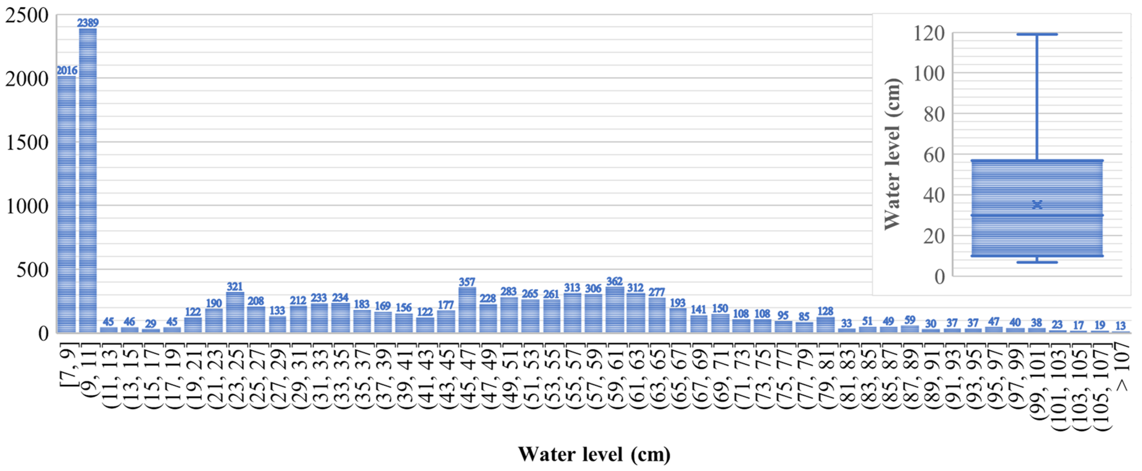
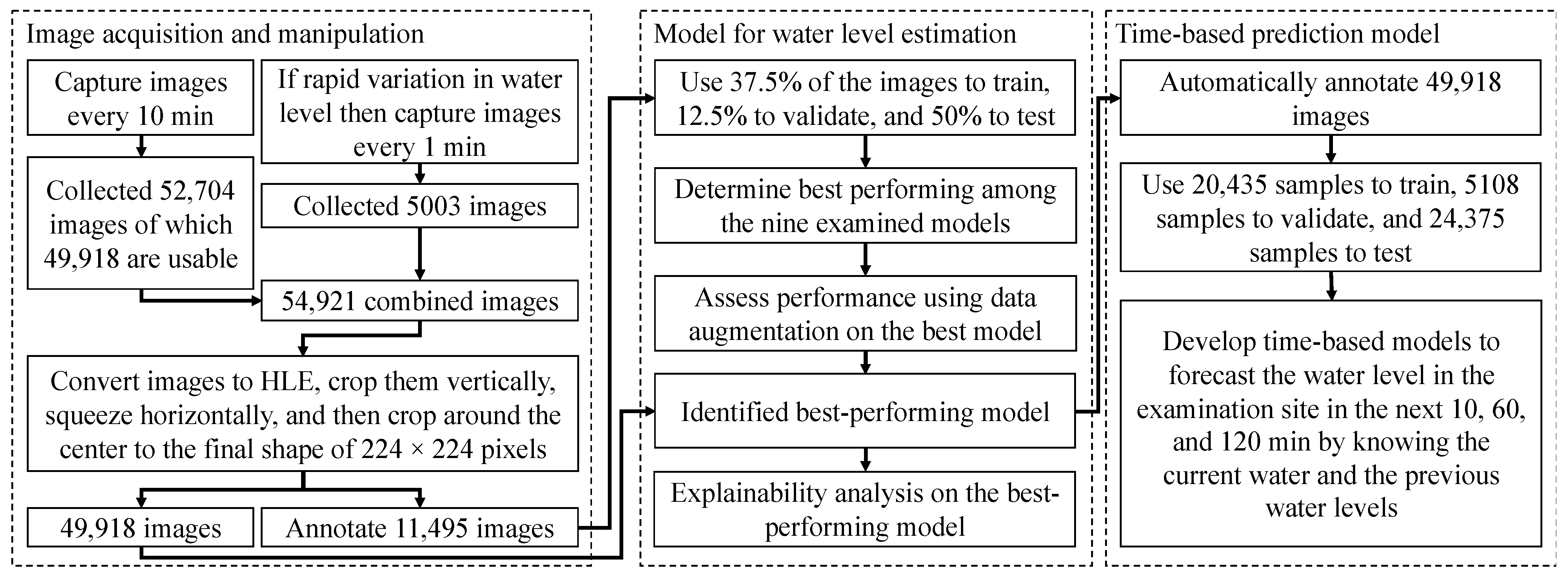
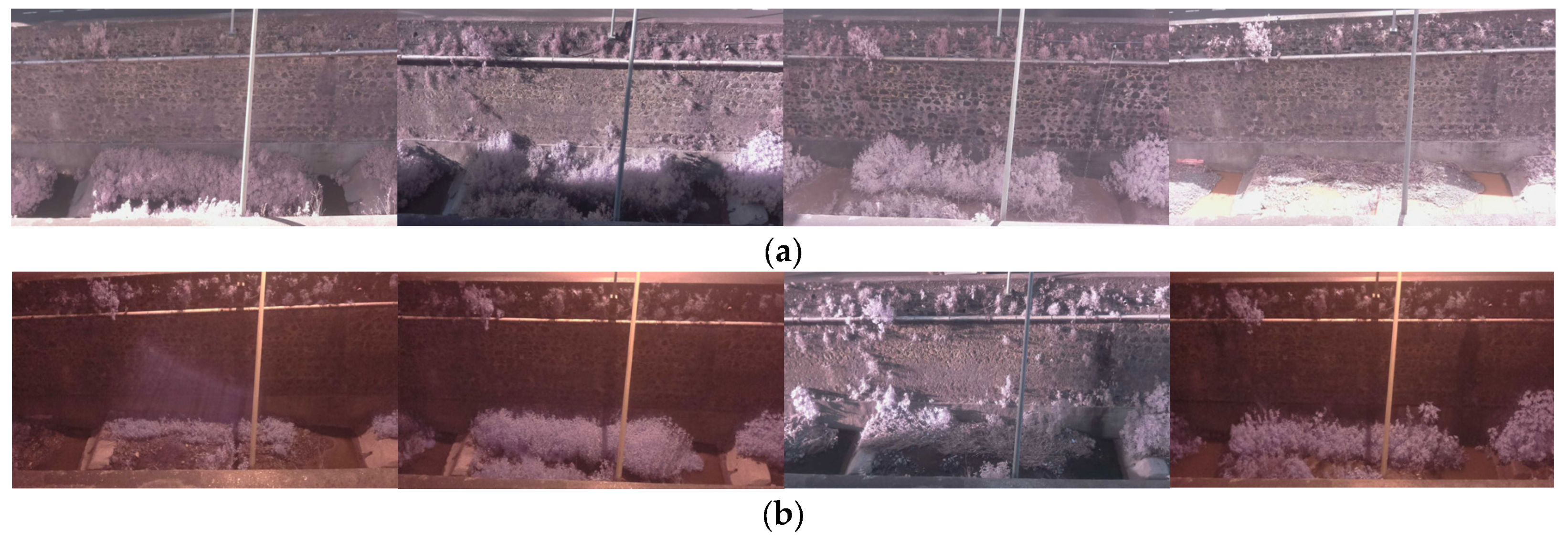
3.3. Data Collection

The developed platform was installed under a balcony of one of the buildings surrounding the monitored water channel, protecting the camera from rain and direct sunlight. The camera was at a distance of 23.7 m from the wall used to measure the water level. A cutting section representing the site installation is shown in Figure 2. The collected images monitored the channel without capturing the information from the public streets.
A database was created by capturing images from the water channel during the entire year (from January to December) of 2020. The hardware could capture an image with a periodicity of 1 min. Thus, a total of 527,040 images could be collected. However, due to power constraints and taking into account the usual slow variation in the water level, the images were collected over a 10 min period. This also aligns with the Portuguese Institute of the Sea and the Atmosphere weather-based practices in Madeira [34]. Therefore, 52,704 images were collected; however, due to internet-based problems and image corruption, the total amount of usable pictures was 49,918. To attain a better resolution in the water-level changes, during the rapid variations in the levels, the periodicity during these events was reduced to 1 min. A total of 5003 images were additionally collected, leading to a total number of captured images of 57,707, of which 54,921 were usable.
The water-level annotation was carried out using a combination of a semi-automatic technique developed by [7] with the subsequent manual supervision of all images to correct the errors. The ground truth for the annotation was based on preliminary measurements from a ruler, examining the highlighted location presented in Figure 3. However, the annotation procedure was laborious and time-consuming. Hence, it was unfeasible to annotate all the images. Thus, from all the captured images over the year, 11,495 were selected for the dataset, not including most photos where the water level was below 10 cm, the most usual value during the year, while keeping most of the samples above this level. The rationale for this dataset was to make the models focus on the highest water levels as they were the most relevant for flooding.
The data distribution is shown in Figure 4. This dataset was made publicly available with the Digital Object Identifier (DOI) at Mendonça, Fábio (2023), “Madeira Water Channel”, Mendeley Data, V2, DOI: 10.17632/bkn36h64ts.2, allowing other researchers to further confirm the results attained by this work and improve them. Statistical measures of the dataset water level are presented in Table 1, including the specifications for the day and nighttime, adjusted daily for Funchal, and including the daylight-saving time.

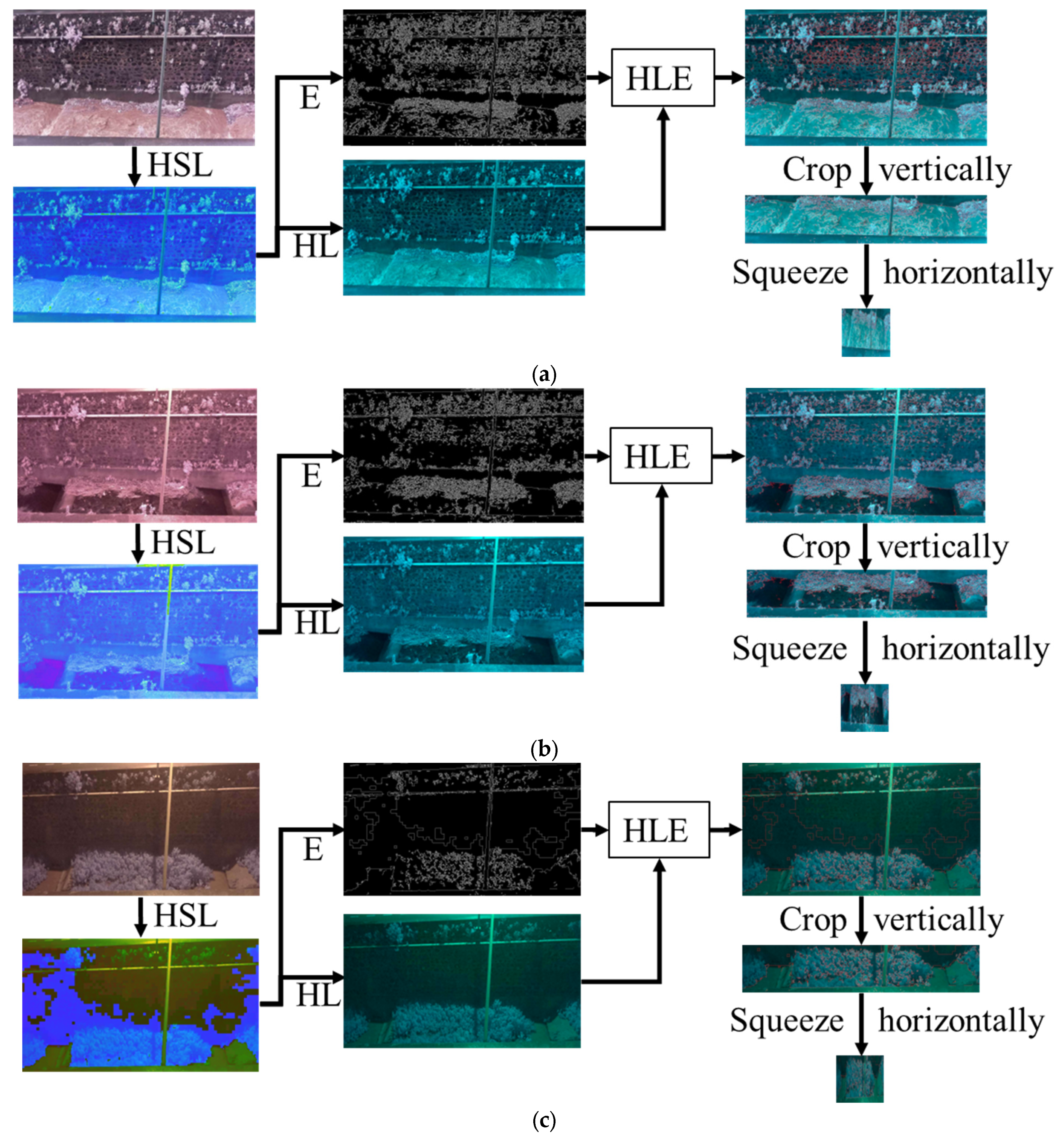
3.4. Image Processing

Image normalization, using the Min–Max method [35], was applied to the stored images to increase the image contrast, assisting the regression model in extracting features from the image. Following a similar approach used by Xu et al. [10], the color space of the images was changed to HSL. This color space presents immunity to alterations in the illumination [36], which is required for the monitored location where the illumination varies during the day. Additionally, it was observed that the saturation component was not relevant for the examined images and even clouded the pictures during the night operation. Therefore, this component was replaced by edge detection, which was used since it was recommended by state-of-the-art works to stress the water line. However, in this work, it was also used to emphasize elements that the regression model should ignore, such as vegetation, turbulent water, and debris on the water’s surface. Therefore, the HLE color space was produced. The Canny algorithm [37] was used for edge detection as it was reported to be suitable for water-level detection in state-of-the-art works [7].
The image was cropped to accommodate the maximum water level of the dataset (120 cm) and to match the regression model’s requirements. Therefore, the pictures were cropped at 256 pixels in height (counting from the bottom). This method was preferred to squeeze vertically since it could maintain the vertical resolution of the images, affecting the minimum pixel height (for the employed image resolution, it was estimated to range from 1.93 to 1.8 cm when the water level rose from 7 to 120 cm, respectively). This approach also has the advantage of deleting unnecessary information about the wall patterns that can confuse the model. Lastly, the image was squeezed horizontally to 256 pixels in width, matching the dimensions the employed regression model needed. The squeezing operation was used since the horizontal resolution was less relevant than keeping the complete (uncropped) water line in the image. Finally, the image was cropped around the center to the final size of 224 × 224 pixels.
Figure 5 depicts four examples of processed images, each at a different time during the day and with varying water levels. It is possible to observe in (a) a picture of a daytime operation in a turbulent stream with a water level above average. Furthermore, the water ripples (that should be ignored) and the water line (that must be detected) are highlighted by edge detection. It is also known that removing the saturation component does not substantially alter the image patterns, maintaining the most relevant information for the model. A similar conclusion can be reached for (b), where the different colors in the original image that are generated in the evening twilight are noticeable, in this case, with a quiet water stream with a level below the average and vegetation highlighted by edge detection. Lastly, (c) depicts a stream with the lowest water level at night, where the water channel is illuminated by streetlamps (mounted on the water channel wall), with vegetation and water level visibly marked by edge detection. In this last image, the problem of using saturation is noticeable, as it clouds the image. The objective of edge detection is to emphasize vegetation and water ripples that should be ignored, while simultaneously delineating the water line (requiring detection). We anticipate that this approach will enhance the model’s understanding of image characteristics.

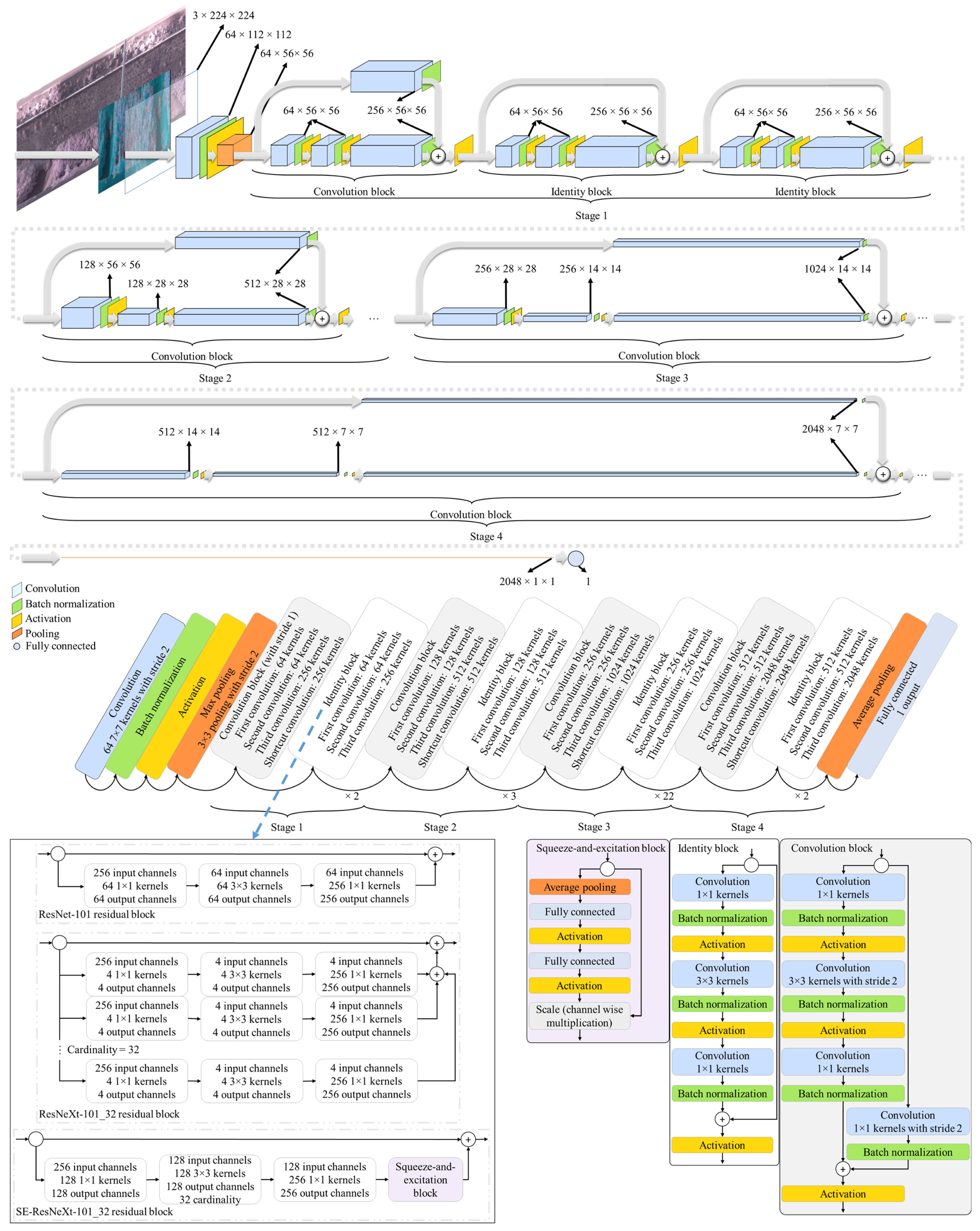
3.5. Model for Water-Level Estimation

Since the problem required a continuous output of the water-level estimation, a regression-based model was thus needed. The developed regression model was based on ResNet architecture, recommended in the state of the art for regression with images [28]. Therefore, multiple variants of this architecture were examined to assess those more suitable for this work. Particularly, versions with 50, 101, and 152 layers were evaluated, using version 1.5 as it was shown to outperform version 1, and the model was initialized following the approach defined by He et al. [38]. The standard version with 18 layers was also studied. Performing depth scaling (increasing the number of layers) was expected to improve the performance. However, when using deeper architectures, gradient-related problems occur, causing the performance gain to become marginal [39]. Hence, it is likely that using even deeper ResNet architectures will not justify the performance-to-complexity ratio.
Figure 6 shows the employed ResNet-101 architecture, where we introduced the last fully connected (dense) layer to produce the regression output. In the first section, denoted as the input stream, a 7 × 7 convolution with 64 kernels (feature maps), a stride of 2, and a padding of 3, allowed reducing the input image size from 224 × 224 to 112 × 112 pixels while the channel depth increased from 3 to 64. The convolution layer output was further reduced to 56 × 56 pixels by a subsampling layer performing a 3 × 3 maximum pooling operation with a stride of 2. A sequence of four stages continued to perform this process of lowering the height and width while increasing the depth using bottleneck architecture. Each stage was composed of a residual block series, containing the bottleneck that, in turn, was a sequence of three convolution layers performing 1 × 1, 3 × 3, and 1 × 1 convolution operations.
The third convolution layer had four-times the number of kernels from the previous two, while the second convolution layer reduced to half the image height and width. This allowed us first to reduce and then expand the depth, making it possible to increase the number of kernels while reducing the computational cost of calculating the 3 × 3 convolution. The number of kernels was chosen so that it doubled per stage, starting with 64, 64, and 256 (in the first stage) and finishing with 512, 512, and 2048 (in the fourth stage). ResNet-50 and ResNet-152 have a similar architecture to ResNet-101. However, in the third stage, instead of 22 identity blocks, the first had 5, while the second had 35. Furthermore, in the second stage, ResNet-152 had 7 identity blocks instead of 3. As a result, the numbers of blocks in the four stages were 3, 4, 6, and 3 for ResNet-50; 3, 4, 23, and 3 for ResNet-101; and 3, 8, 36, and 3 for ResNet-152.
In each residual block, the first two convolution layers of the bottleneck were followed by batch normalization and activation. The first biased the residual blocks toward the identity function, allowing the training of deeper networks [40]. The second introduced a nonlinearity, and the standard Rectified Linear Unit (ReLU) was used. However, the last convolution layer was only followed by batch normalization, and its output was combined with the shortcut (skip) connection. This outcome was then passed by an activation, resulting in the residual block output. This shortcut connection allows identity mapping, which is why deep residual neural networks can increase the number of layers without reducing their performance due to gradient-related problems during training [41]. These residual blocks are denoted as identity blocks. However, when there is image reduction, the shortcut connection needs to be adjusted so that it can be combined with the bottleneck output. Therefore, a 1 × 1 convolution followed by batch normalization is used to perform a linearly transformed shortcut connection, using the same number of kernels as the last convolution layer of the bottleneck. These blocks are denoted as convolution blocks.
The first stage receives the input stream’s output and is composed of a convolution block followed by two identity blocks. The second stage starts with a convolution block; however, the bottleneck’s middle convolution layer and the shortcut convolution layer employ a stride of 2 to reduce the image size. Later, three identity blocks are used. The two subsequent stages are similar, but use five and two identity blocks, respectively. Therefore, the ResNet architecture allows doubling the number of channels (channel width) while reducing the image size by half from one stage to another.
ResNet-18 also has four stages with a concept similar to the other examined architectures. However, each stage comprises two blocks; the first is a convolution block followed by an identity block. Furthermore, the bottleneck comprises two convolution layers, both performing 3 × 3 convolution operations. Batch normalization is used after the convolution layers, and activation is employed after the first batch normalization. In the same way as the other examined architectures, the second batch normalization output is combined with the shortcut connection, whose output is then passed by an activation, creating the residual block output. The numbers of kernels used in the convolution layers of the bottleneck were 64, 128, 256, and 512 for stages one to four, respectively [38]. As a result, the output shape of all examined ResNet stages and output layer were the same, being 56 × 56, 28 × 28, 14 × 14, 7 × 7, and 1 × 1.
In addition to the standard ResNet architecture, three state-of-the-art advances were examined, which could lead to a better performance [42]. The first, named ResNeXt, used a split–transform–merge strategy and was shown to outperform other state-of-the-art architectures, such as standard ResNet, Inception-v3, and Inception-ResNet-v2. ResNeXt uses multiple filters that operate at the same level in a multi-branch architecture. Following Xie et al. [42], two architectures were examined, with a cardinality (number of branches) of 32; the first is based on ResNet-50, while the second is based on ResNet-101. Therefore, the input channels were divided into 32 groups that fed the parallel stacking of convolution operations whose outputs were then combined. It was observed that increasing cardinality could lead to better results than having a deeper or wider architecture [42]. Furthermore, two standard values for the bottleneck width (4 and 8) were also examined.
The second examined alteration was Squeeze and Excitation (SE), which adds an attention module to the architecture that can lead to significant performance improvements [43]. This attention mechanism allows the recalibration of channel-wise features adaptively by modeling the channels’ interdependencies. First, it performs a squeezing operation to produce a channel descriptor, followed by excitation, which generates the per-channel modulation weights. Particularly, the squeezing operation performs a global average pooling to pool the most informative feature that will act as a channel descriptor since the output shape is 1 × 1 × number of channels. Subsequently, two fully connected layers introduce parameterization allowing the model to learn the nonlinear interaction between channels. The first fully connected layer uses ReLU as an activation function and reduces the output channel complexity (the number of neurons is given by the number of channels/ratio, using 16 as the default value for ratio), while the second fully connected layer uses sigmoid as an activation function, restoring the original complexity (the number of neurons is equal to the number of channels) and allowing each channel to be emphasized. The created output is then fed to the excitation part, which weighs each feature map provided to the squeeze-and-excitation block.
The last examined alteration was the Wide ResNet (W_ResNet), as width scaling was reported to be a capable alternative to depth scaling [39]. Particularly, the examined W_ResNet only modified the number of channels in the 3 × 3 convolutions by doubling its value.
All code was developed in Python 3 using PyTorch version 1. Transfer learning was used to bypass the need for large data volumes when developing deep learning models [29]. In this work, the examined models were pre-trained in the ImageNet-1K database, which comprised 1,281,167 training images and 1000 categories [44].
The pre-trained models were retrained in the developed database by adding a fully connected layer with one unit as the output layer to produce the regression output. Adaptive Moment (ADAM) [45] estimation was used for the stochastic optimization of the retraining procedure with a learning rate of 0.0001. Early stopping was employed to avoid overfitting, stopping the training procedure (before the limit of 200 epochs) if a succession of 10 epochs occurred where the improvement in the tracked metric was less than 0.01.

3.6. Time-Based Prediction Model

With the goal of forecasting possible flood events, a Nonlinear Autoregressive Exogenous (NARX) model was developed to forecast the water level in the future. It is based on a recurrent neural network with feedback connections and has fast convergence with good generalization [46,47]. Moreover, this model was previously shown to be suitable for forecasting complex time series regarding flooding events [48]. Therefore, this model was used in the time-based analysis.
A standard NARX architecture was used, considering a network with two layers and 100 hidden units. Additionally, a lag of 12 inputs was used, denoting a delay of 120 min (10 min per sample). The processing flow used for time-based prediction is presented in Figure 7, where it is possible to observe that the ResNet model examines the figures to make the water-level estimations that influence the NARX to make future forecasts. Three NARX models were developed to forecast the water levels in the following 10 min, 60, and 120 min. Such predictions can then be potentially used for flood risk assessment.
It is imperative to consider that various segments of the water channel can exhibit different water levels during flooding, owing to variations in channel characteristics and population density along its length. Consequently, the decision was made to develop a water-level estimation model rather than a flood/non-flood classification system. Each forecasting interval served a distinct purpose: the 10 min forecast offered immediate insights crucial for prompt responses during sudden situations, while the 60 min forecast provided a medium-term perspective, aiding in comprehensive planning and resource allocation. Extending the lead time, the 120 min forecast facilitated the improved organization of evacuation efforts and the preparation of shelters. Given Madeira’s unique topography and susceptibility to rapid environmental shifts, shorter forecasting intervals hold particular significance and can be more pertinent than longer ones in effectively addressing dynamic conditions. Additionally, it is essential to evaluate the readiness of evacuation routes [49], which are likely as relevant as the warning period itself.

3.7. Performance Metrics

Standard regression performance metrics were used to assess the developed models’ performance and allow a comparison with state-of-the-art works. Particularly, the MAE, MAPE, MSE, ME, and Root Mean Squared Error (RMSE) were used [50]. Furthermore, the MSE was used for both tracking the early stopping procedure and as the loss function during training. The performance-to-complexity ratio was also examined to determine if it was worth proceeding toward more complex models (models with more parameters). This ratio was defined as (1 − MAPE)/number of parameters.

4. Results and Discussion

Data were randomly divided into two for all tests, keeping half of the data for training and the other half for testing. Furthermore, 25% of the training dataset was held to produce a validation dataset (thus, 12.5% of the total data was used for validation), and the batch size was set to 8. The implemented pipeline is presented in Figure 8. First, a database was created from the acquired images, which was then used to assess the performance of the examined regression models. The best-performing model was then further investigated by carrying out an explainability analysis. Lastly, the water channel was modeled to develop a model capable of forecasting the future by knowing the current and previous water levels in the examination site.

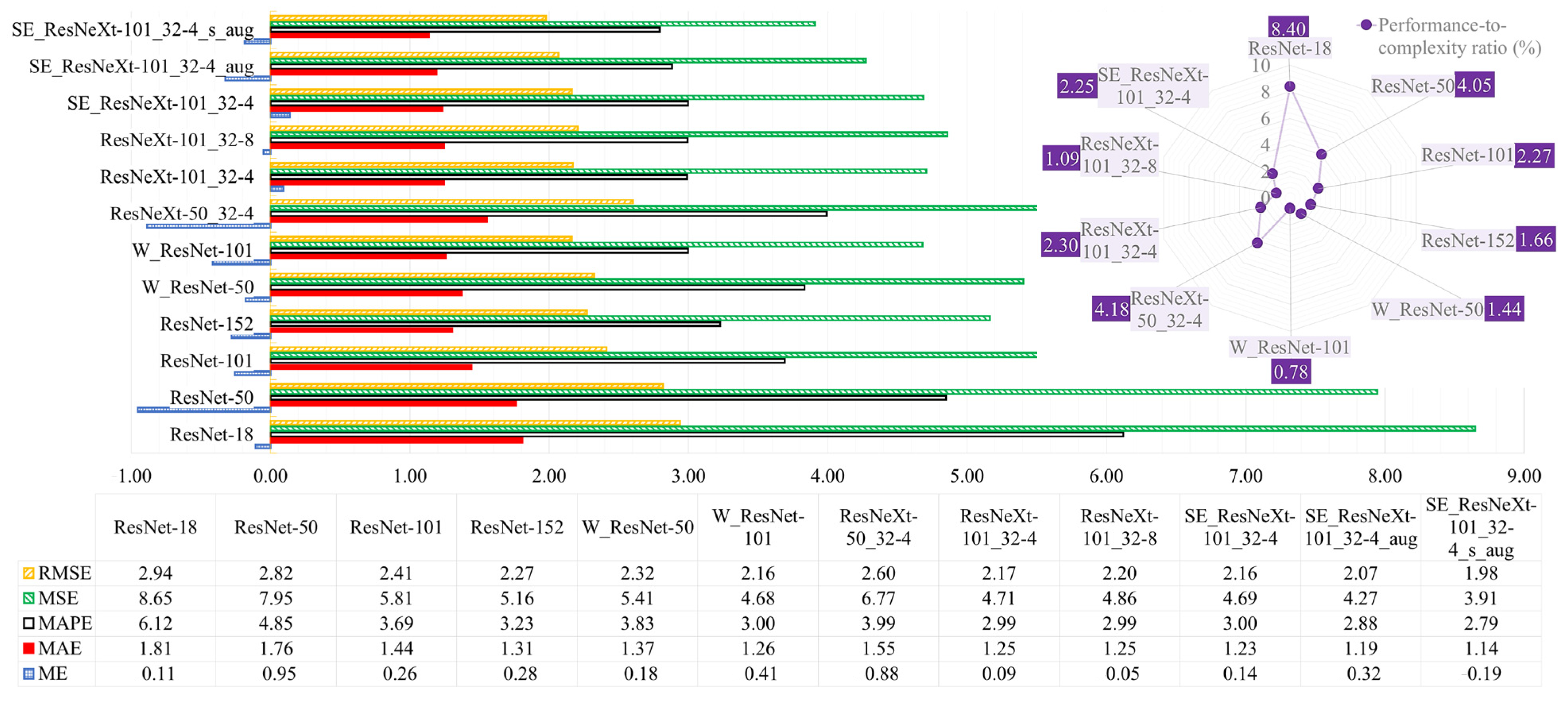
4.1. Water-Level Estimation

The performance of the four standard ResNet models (ResNet-18, ResNet-50, ResNet-101, and ResNet-152) was initially assessed, and Figure 9 presents the performance metrics of the examined architectures. The continuous reduction in error metrics is notorious when depth scaling is performed from ResNet-18 to ResNet-152. However, as depicted in Figure 9, the performance-to-complexity ratio continuously reduces, with ResNet-152 attaining the worst result, suggesting a saturation in the depth scaling. Hence a compromise between performance and complexity was considered, focusing the subsequent analysis on the 50 and 101 architectures.
It was observed that using W_ResNet substantially increased the performance compared to standard ResNet, although the performance-to-complexity ratio was lower. Furthermore, ResNeXt-101 attained a better performance (lower error metrics) with a better performance-to-complexity ratio than W_ResNet-101. Moreover, a bottleneck width of 4 or 8 yielded the same performance; thus, ResNeXt-101_32-4 is preferable (it has a better performance-to-complexity ratio). Therefore, the SE attention module was applied to the best-performing model (ResNeXt-101_32-4), achieving a better performance while improving the performance-to-complexity ratio.
Finally, data augmentation was applied to the training data by doubling their size, and the best-performing model was trained on these new data. Notably, each sample of the training dataset was copied, and then the augmentation procedure was applied to the copied image. This way, both original and augmented images were presented to the model during training. Two augmentation procedures were examined. The first was using the standard AutoAugment from ImageNet (the resulting performance was identified with aug at the end) [51], which applies numerous procedures to modify the images substantially. However, the examined problem was a water channel monitored by a camera in a fixed location, which mostly suffered through time from slight rotations and shifts in the images, and from the variation in the light intensity (from day to nighttime over the year). Therefore, the second examined augmentation procedure was proposed in this work by performing minor augmentations that stressed the mentioned effects. Specifically, each copied image had a 50% probability of being solarized; then, random color jitter was applied to the brightness, contrast, saturation, and hue. Finally, the images were randomly rotated in the −20° to 20° range. The resulting performance was identified with s_aug at the end.
It was observed that both data augmentation procedures further decreased the error while keeping the same performance-to-complexity ratio. In addition, the proposed augmentation method led to the best-performing model, with an MAE of 1.14 cm. Furthermore, when checking the day and night images, it was observed that the MAE was slightly higher in the day images (1.20 cm) than in the night ones (1.09 cm). The prediction errors are shown in Figure 10, where the error line points to one outliner sample. It is also noticeable that the tendency line has almost a 45° slope with an R2 of nearly 1, strongly supporting the claim that the model’s forecasts have a lower error.
An outlier analysis was carried out, and the highest error occurred on 19 October 2020, at 5:41 a.m. Further investigation revealed an anomalous water stream directly above the region of interest, originating from an underground pipe beneath the street. This led the model to inaccurately predict a higher water level in the image. Notably, a similar phenomenon caused high errors on the same day on other samples. Upon removing the sample, we observed no significant impact on the MAE. We attributed this lack of effect to the substantial sample size. Therefore, we decided to retain these images in the dataset to maintain a diverse range of occurrences. It is also important to note that this occurrence shows that the model is indeed examining the region of interest to make the forecasts.
A direct comparison with other state-of-the-art works is problematic since only one other work [7] has examined the type of water channels evaluated in this work. However, an estimate can be attained by considering the capability of the models to predict the water level. Azevedo and Brás [7] reported average MAEs of 1.8 cm and 2.8 cm during the day and nighttime images, respectively. It is possible to conclude that the day error is higher than the value of this work (1.20 cm); furthermore, the nighttime error is substantially larger than the attained performance (1.09 cm), advocating the preeminence of the proposed models to adapt to the changing operating conditions during the day. Additionally, the other previously discussed state-of-the-art works reported an error in the same range or higher than the error attained in this work, supporting the significance of the developed model.

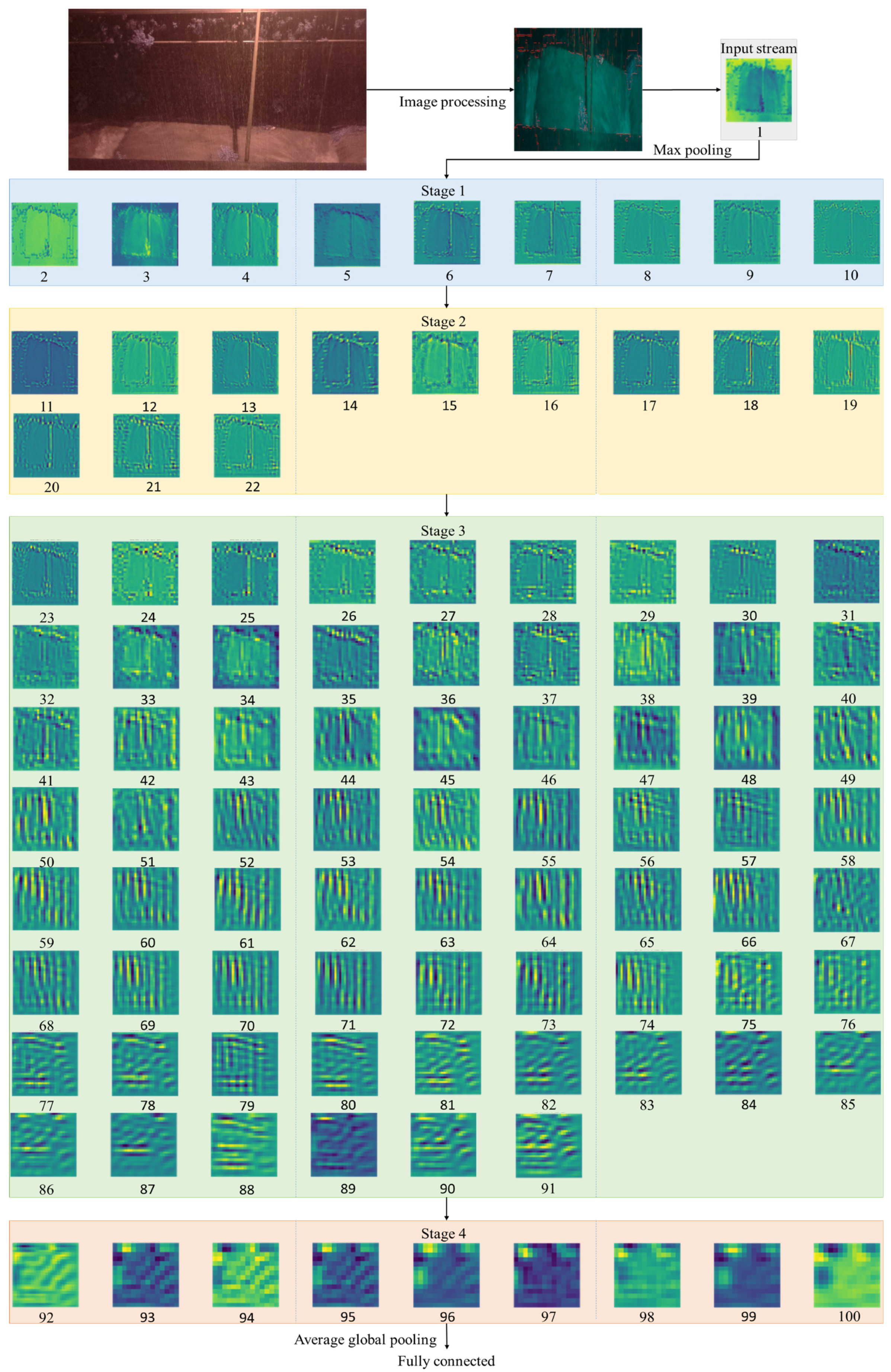
4.2. Explainability of the Model

A common problem with using machine learning algorithms is the lack of explainability of the models, as they are operated as a black box [52]. This issue is particularly prominent in models based on deep neural networks, as the extracted features become more complex as we travel deeper into the models’ layers. Hence, an effort to attain a transparency approach was carried out in this work with visual explanations by example, leading to an opaque model. This analysis was carried out on the best-performing model (SE_ResNeXt-101_32-4_s_aug).
For this purpose, two approaches were employed. The first evaluated the feature maps created by each convolution layer of the model (the ones in the shortcut connection were not considered as they are used for keeping the shapes) when an image was presented. In contrast, the second examined the Gradient-weighted Class Activation Mapping plus plus (Grad-CAM++) [53] applied to the model when an image was fed to identify the image patterns that impacted the model’s predictions the most. Furthermore, Grad-CAM++ analysis was carried out through the progress of the model’s training, allowing us to observe where the model focus shifted during the learning procedure.
Figure 11 presents the created feature maps when an image with the highest water level in the database is fed to the model. It is possible to observe that, as we travel deeper into the network, the created features are initially related to the shape and edges, becoming more complex and not humanly understandable in the latter stages. The input stream keeps the primary forms of the image, while in stage 1, it is noticeable that the model is extracting the edges. We hypothesized that the edge component in the produced HLE color space facilitated this process. In stage 2, the model extracts variations in the previously assessed edges; in this case, the bottom wall, the vertical line of the streetlamp, and the water level in the top wall are visible. Especially in convolution layer 18, it is visible that the model ignores the shadow cast by the top wall and identifies the correct water line. In stage 3, the extracted feature becomes progressively more abstract, although it seems like the model first looks for vertical line changes and then for horizontal variations. In the last stage, the created features are challenging to understand, although it seems to look for diagonal variations.
The progress of the best-performing model’s training with an example of a specific image, for which we can observe Grad-CAM++, is presented in Figure 12. The fed image is at the highest water level and without vegetation, where we can see the model focuses on the overall water region. We can observe that the model learned to focus on reference elements, such as the top wall patterns, the vertical streetlamp, and the area where the water level is visible. In the second image, the water level is above the average (61 cm) with some vegetation, where we can see the model ignoring the vegetation. The last fed image is at the lowest water level (7 cm) with extensive vegetation, in which we can observe the model ignoring the vegetation cluster, focusing on its borders and the water-level mark on the top wall. Figure 11 and Figure 12 demonstrate that the model predominantly focuses on the water channel’s main structure and the water level, while largely ignoring the vegetation. As the water channel structure is very similar along the full channel, this robustness in capturing essential features suggests that the model’s performance will likely generalize well to new sites.
Lastly, images that presented to the highest errors were examined to determine their common characteristics. Figure 13a,b present images that present a higher overestimation and underestimation, respectively. A shared trait in all images with considerable overestimations was the presence of a sturdy variation from sunlight to shadow. It appears that when the bottom wall is too much illuminated compared to the water line, the model loses some of its references. In addition, the shadow on the top wall (above the water line) can also lead to an overestimation, where the model identifies this shadow as the water line. On the other hand, a communal characteristic of images that leads to substantial underestimations is the presence of a shadow covering the water line and usually having a darker water color, suggesting that the model can be identifying the shadow as the water line.

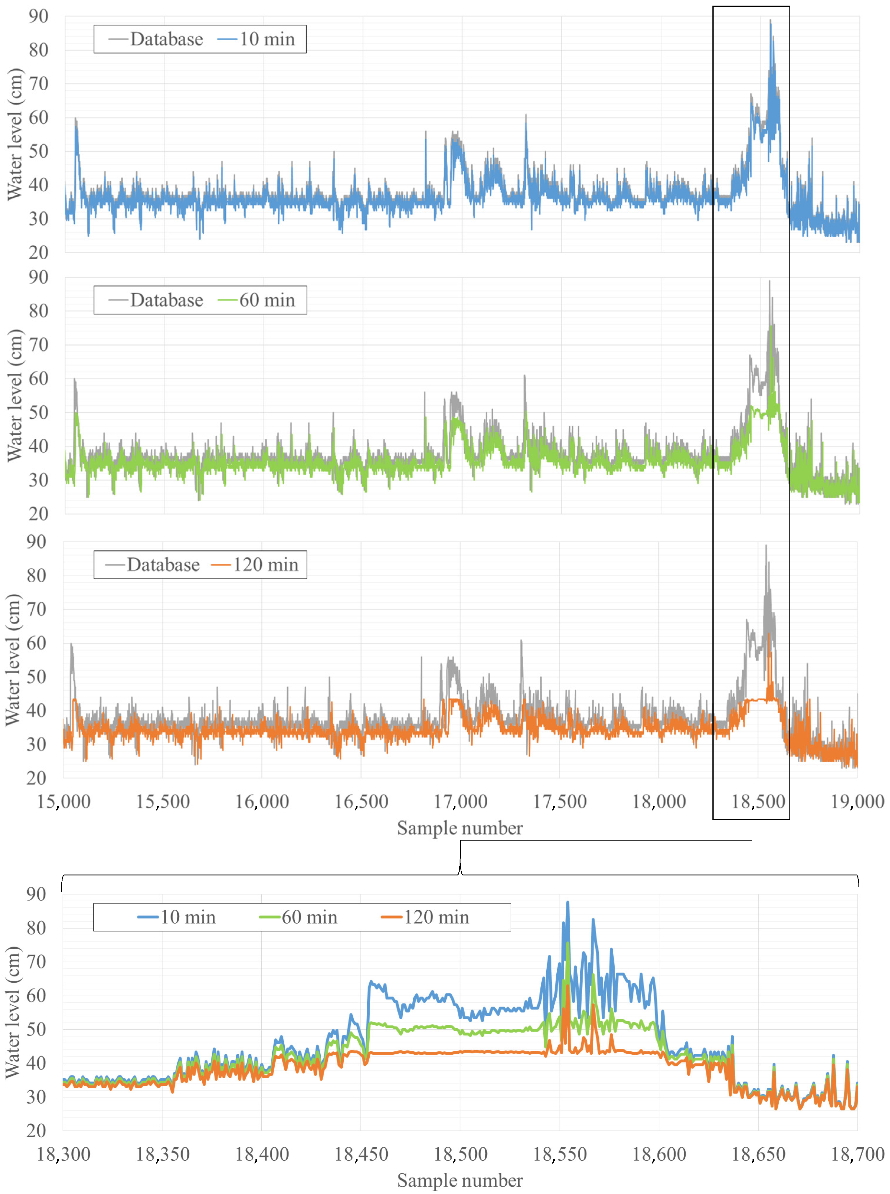
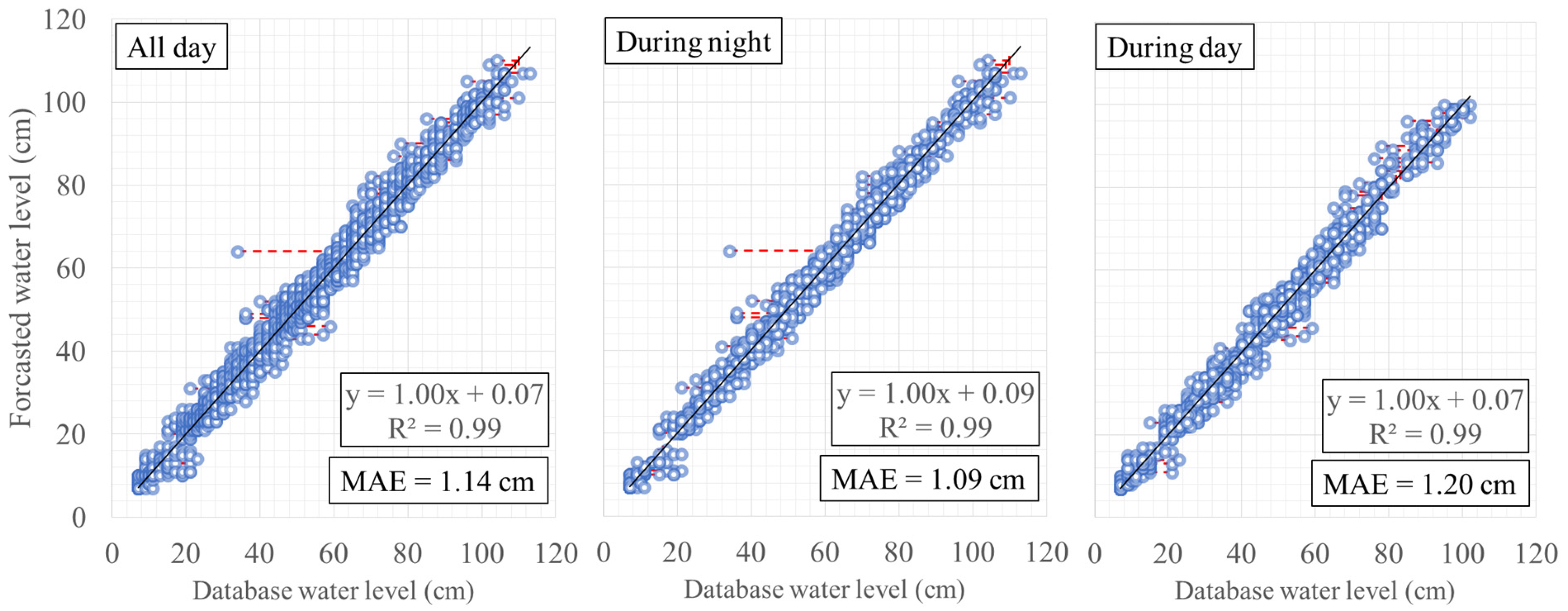
4.3. Forecasting the Water Level

A NARX model was developed to forecast the water levels in the next 10 min, 60, and 120 min. For this purpose, all images collected over the year (except those used for training the model or that were corrupted), at each 10 min period, were considered. This period was used since it matched the one used by the Portuguese Institute of the Sea and the Atmosphere in weather-based analysis. Therefore, the best-performing model (SE_ResNeXt-101_32-4_s_aug) was used to label all these images (this analysis was validated by the low error attained by the model in the performance analysis), creating a time series of the water level with a period of 10 min between samples.
The data from January to June were used to train the model (from 25,543 samples, 20% was used as validation and the remaining for training), and the remaining months were employed for testing (24,375 samples). Throughout the year, water levels showed substantial seasonal changes. November to February experienced increased rainfall, leading to higher water levels, while the remaining months showed more stable flow patterns, with lower levels averaging around 7 cm during summer. We divided the year in half to capture these patterns, aiming to train and validate our model effectively across representative seasonal variations. The MAEs attained for the 10 min, 60 min, and 120 min forecasts were 1.76 cm, 2.09 cm, and 2.34 cm, respectively. It was observed that, during low-water-variation periods, all three models presented similar behavior. However, during fast variations in the water level, the 120 min model produced a high error (it had a greater inertia to make changes), suggesting that it was not worth exceeding 120 min. An example of a fast variation period for the three models is presented in Figure 14, where the previous observation is noticeable. Nevertheless, the model could reliably estimate the water level for at least 60 min; this information can then be used for flooding risk assessments, sounding an alarm if the forecasted water level exceeds a pre-defined limit.

5. Conclusions

A system for measuring the water levels in volcanic islands’ water channels in urban areas was proposed in this work, using machine learning approaches based on deep learning models. For this purpose, the proposed regression model applied transfer learning to multiple ResNet architectures, evaluating images captured by a low-cost remote monitoring system that was converted to the proposed HLE color space.
The best-performing model (SE_ResNeXt-101_32-4_s_aug) attained an MAE that was as good or superior to previous state-of-the-art works while using a fully automated approach that only required images from a single camera without using any ruler to facilitate the estimation. An explainability analysis was then carried out with a visual explanation by example, producing an opaque model. In addition, two approaches were used. The first was based on evaluating the generated feature maps, while the second used Grad-CAM++. An explanation for the occurrence of the more extensive error was also presented, concluding that light conditions and the location of shadows can affect the model’s forecasts.
Lastly, a time-based model was used to model the water channel, allowing us to forecast the water levels in the next 10 min, 60 min, and 120 min. It was observed that 120 min was likely excessive for the forecast since it could not correctly follow fast transitions, while the 10 min mark could easily follow these transitions. The 60 min model, although with some errors, could follow these transitions, creating a potential flooding risk-assessment mechanism. Such a mechanism can be of utmost relevance for volcanic islands’ water channels, where floods can devastate urban areas.
The main limitation of this work was the use of data from only one year to develop all the models; hence, a future direction is to continuously acquire and annotate data, allowing the development of further robust models. Likewise, the time-based model can be further improved by these additional data. It is also important to examine the transferability of the model to other locations of the water channel. Similarly, it would be relevant to examine locations with a well-defined flooding season to test the suitability of flooding detection. Lastly, it is relevant to study other baseline models for time-series forecasting for comparison purposes and to include environmental variables (such as temperature and humidity) in the modeling approach to further extend the forecast window.

Author Contributions

Conceptualization, F.M., S.S.M. and J.A.A.; methodology, F.M. and S.S.M.; software, F.M., S.S.M. and J.A.A.; validation, F.M., S.S.M., F.M.-D., J.A.A., A.G.R.-G. and J.L.N.-M.; formal analysis, F.M., S.S.M., F.M.-D., J.A.A., A.G.R.-G. and J.L.N.-M.; investigation, F.M., S.S.M., F.M.-D., J.A.A., A.G.R.-G. and J.L.N.-M.; resources, J.A.A.; data curation, F.M. and J.A.A.; writing—original draft preparation, F.M.; writing—review and editing, S.S.M., F.M.-D., J.A.A., A.G.R.-G. and J.L.N.-M.; visualization, F.M.; supervision, F.M.-D., J.A.A., A.G.R.-G. and J.L.N.-M.; project administration, F.M. and J.A.A.; funding acquisition, J.A.A., A.G.R.-G. and J.L.N.-M. All authors have read and agreed to the published version of the manuscript.

Funding

This research was funded by ARDITI—Agência Regional para o Desenvolvimento da Investi-gação, Tecnologia e Inovação under the scope of the project M1420-09-5369-FSE-000002—Post-Doctoral Fellowship, co-financed by the Madeira 14-20 Program—European Social Fund. This research was funded by LARSyS (Project UIDB/50009/2020, DOI 10.54499/UIDB/50009/2020 (https://doi.org/10.54499/UIDB/50009/2020)). This research was partially supported by the Center for Research in Mathematics and Applications (CIMA) related with the Statistics, Stochastic Processes and Applications (SSPA) group, through grant UIDB/04674/2020 from FCT–Fundação para a Ciência e a Tecnologia, Portugal (https://doi.org/10.54499/UIDB/04674/2020).

Data Availability Statement

All the data are available at https://doi.org/10.17632/bkn36h64ts.2 (accessed on 19 January 2024).

Conflicts of Interest

The authors declare no conflicts of interest.

References

  1. Döll, P.; Jiménez-Cisneros, B.; Oki, T.; Arnell, N.; Benito, G.; Cogley, J.; Jiang, T.; Kundzewicz, Z.; Mwakalila, S.; Nishijima, A. Integrating Risks of Climate Change into Water Management. Hydrol. Sci. J. 2015, 60, 4–13. [Google Scholar] [CrossRef]
  2. Zhen, Y.; Liu, S.; Zhong, G.; Zhou, Z.; Liang, J.; Zheng, W.; Fand, Q. Risk Assessment of Flash Flood to Buildings Using an Indicator-Based Methodology: A Case Study of Mountainous Rural Settlements in Southwest China. Front. Environ. Sci. 2022, 10, 931029. [Google Scholar] [CrossRef]
  3. Vieira, I.; Barreto, V.; Figueira, C.; Lousada, S.; Prada, S. The Use of Detention Basins to Reduce Flash Flood Hazard in Small and Steep Volcanic Watersheds—A Simulation from Madeira Island. J. Flood Risk Manag. 2018, 11, S930–S942. [Google Scholar] [CrossRef]
  4. Bradley, A.; Kruger, A.; Meselhe, E.; Muste, M. Flow Measurement in Streams Using Video Imagery. Water Resour. Res. 2002, 38, 1315. [Google Scholar] [CrossRef]
  5. Loizou, K.; Koutroulis, E. Water Level Sensing: State of the Art Review and Performance Evaluation of a Low-Cost Measurement System. Measurement 2016, 89, 204–214. [Google Scholar] [CrossRef]
  6. Yorke, T.; Oberg, K. Measuring River Velocity and Discharge with Acoustic Doppler Profilers. Flow Meas. Instrum. 2002, 13, 191–195. [Google Scholar] [CrossRef]
  7. Azevedo, A.; Brás, J. Measurement of Water Level in Urban Streams under Bad Weather Conditions. Sensors 2021, 21, 7157. [Google Scholar] [CrossRef] [PubMed]
  8. Gleason, C.; Smith, L.; Finnegan, D.; LeWinter, A.; Pitcher, L.; Chu, V. Semi-Automated Effective Width Extraction from Time-Lapse RGB Imagery of a Remote, Braided Greenlandic River. Hydrol. Earth Syst. Sci. 2015, 19, 2963–2969. [Google Scholar] [CrossRef]
  9. Bandini, F.; Jakobsen, J.; Olesen, D.; Reyna-Gutierrez, J.; Bauer-Gottwein, P. Measuring Water Level in Rivers and Lakes from Lightweight Unmanned Aerial Vehicles. J. Hydrol. 2017, 548, 237–250. [Google Scholar] [CrossRef]
  10. Xu, Z.; Feng, J.; Zhang, Z.; Duan, C. Water Level Estimation Based on Image of Staff Gauge in Smart City. In Proceedings of the 2018 IEEE SmartWorld, Ubiquitous Intelligence & Computing, Advanced & Trusted Computing, Scalable Computing & Communications, Cloud & Big Data Computing, Internet of People and Smart City Innovation (SmartWorld/SCALCOM/UIC/ATC/CBDCom/IOP/SCI), Guangzhou, China, 8–12 October 2018. [Google Scholar]
  11. Caliskan, E. Environmental Impacts of Forest Road Construction on Mountainous Terrain. Iran. J. Environ. Health Sci. Eng. 2013, 10, 23. [Google Scholar] [CrossRef]
  12. Chen, G.; Bai, K.; Lin, Z.; Liao, X.; Liu, S.; Lin, Z.; Zhang, Q.; Jia, X. Method on Water Level Ruler Reading Recognition Based on Image Processing. Signal Image Video Process. 2021, 15, 33–41. [Google Scholar] [CrossRef]
  13. Guo, S.; Zhang, Y.; Liu, Y. A Water-Level Measurement Method Using Sparse Representation. Autom. Control Comput. Sci. 2020, 54, 302–312. [Google Scholar]
  14. Zhang, Z.; Zhou, Y.; Liu, H.; Gao, H. In-Situ Water Level Measurement Using NIR-Imaging Video Camera. Flow Meas. Instrum. 2019, 67, 95–106. [Google Scholar] [CrossRef]
  15. Zhang, Z.; Zhou, Y.; Liu, H.; Zhang, L.; Wang, H. Visual Measurement of Water Level under Complex Illumination Conditions. Sensors 2019, 19, 4141. [Google Scholar] [CrossRef] [PubMed]
  16. Hies, T.; Babu, P.; Wang, Y.; Duester, R.; Eikaas, H.; Meng, T. Enhanced Water-Level Detection by Image Processing. In Proceedings of the 10th International Conference on Hydroinformatics, Hamburg, Germany, 14 July 2012. [Google Scholar]
  17. Lin, Y.; Lin, Y.; Han, J. Automatic Water-Level Detection Using Single-Camera Images with Varied Poses. Measurement 2018, 127, 167–174. [Google Scholar] [CrossRef]
  18. Pan, J.; Yin, Y.; Xiong, J.; Luo, W.; Gui, G.; Sari, H. Deep Learning-Based Unmanned Surveillance Systems for Observing Water Levels. IEEE Access 2018, 6, 73561–73571. [Google Scholar] [CrossRef]
  19. Qiao, G.; Yang, M.; Wang, H. A Water Level Measurement Approach Based on YOLOv5s. Sensors 2022, 22, 3714. [Google Scholar] [CrossRef]
  20. Ran, Q.; Li, W.; Liau, Q.; Tang, H.; Wang, M. Application of an Automated LSPIV System in a Mountainousstream for Continuous Flood Flow Measurements. Hydrol. Process. 2016, 30, 3014–3029. [Google Scholar] [CrossRef]
  21. Stumpf, A.; Augereau, E.; Delacourt, C.; Bonnier, J. Photogrammetric Discharge Monitoring of Small Tropical Mountain Rivers: A Case Study at Rivière Des Pluies, Réunion Island. Water Resour. Res. 2016, 52, 4550–4570. [Google Scholar] [CrossRef]
  22. Udomsiri, S.; Iwahashi, M. Design of FIR Filter for Water Level Detection. Int. Sch. Sci. Res. Innov. 2008, 2, 2663–2668. [Google Scholar]
  23. Ridolfi, E.; Manciola, P. Water Level Measurements from Drones: A Pilot Case Study at a Dam Site. Water 2018, 10, 297. [Google Scholar] [CrossRef]
  24. Eltner, A.; Elias, M.; Sardemann, H.; Spieler, D. Automatic Image-Based Water Stage Measurement for Long-Term Observations in Ungauged Catchments. Water Resour. Res. 2018, 54, 10362–10371. [Google Scholar] [CrossRef]
  25. Young, D.; Hart, J.; Martinez, K. Image Analysis Techniques to Estimate River Discharge Using Time-Lapse Cameras in Remote Locations. Comput. Geosci. 2015, 76, 1–10. [Google Scholar] [CrossRef]
  26. Eltner, A.; Bressan, P.; Akiyama, T.; Gonçalves, W.; Junior, J. Using Deep Learning for Automatic Water Stage Measurements. Water Resour. Res. 2021, 57, e2020WR027608. [Google Scholar] [CrossRef]
  27. Vandaele, R.; Dance, S.; Ojha, V. Deep Learning for Automated River-Level Monitoring through River-Camera Images: An Approach Based on Water Segmentation and Transfer Learning. Hydrol. Earth Syst. Sci. 2021, 25, 4435–4453. [Google Scholar] [CrossRef]
  28. Lathuilière, S.; Mesejo, P.; Alameda-Pineda, X.; Horaud, R. A Comprehensive Analysis of Deep Regression. IEEE Trans. Pattern Anal. Mach. Intell. 2019, 42, 2065–2081. [Google Scholar] [CrossRef]
  29. Zhuang, F.; Qi, Z.; Duan, K.; Xi, D.; Zhu, Y.; Zhu, H.; Xiong, H.; He, Q. A Comprehensive Survey on Transfer Learning. Proc. IEEE 2021, 109, 43–76. [Google Scholar] [CrossRef]
  30. Direcção Reginal de Florestas Plano de Ordenamento e Gestão Da Laurissilva Da Madeira; REDE NATURA 2000; Direcção Reginal de Florestas: Funchal, Portugal, 2009.
  31. Oliveira, R.; Almeida, A.; Sousa, J.; Pereira, M.; Portela, M.; Coutinho, M.; Ferreira, R.; Lopes, S. A Avaliação Do Risco de Aluviões Na Ilha Da Madeira. In Proceedings of the 10° Simpósio de Hidráulica e Recursos Hídricos dos Países de Língua Oficial Portuguesa (10° SILUSBA), Porto de Galinhas, Brasil, 26 October 2011. [Google Scholar]
  32. Prada, S.; Gaspar, A.; Sequeira, M.; Nunes, A.; Figueira, C.; Cruz, J. Disponibilidades Hídricas Da Ilha Da Madeira. In AQUAMAC—Técnicas e Métodos Para a Gestão Sustentável da Água na Macaronésia; Instituto Tecnológico de Canarias, Cabildo de Lanzarote, Consejo Insular de Aguas de Lanzarote: Lanzarote, Spain, 2005; Volume 1. [Google Scholar]
  33. Jolles, J. Broad-Scale Applications of the Raspberry Pi: A Review and Guide for Biologists. Methods Ecol. Evol. 2021, 12, 1562–1579. [Google Scholar] [CrossRef]
  34. IPMA. Área Educativa—Parques Meteorológicos e Equipamentos. 2022. Available online: https://www.ipma.pt/pt/educativa/observar.tempo/index.jsp?page=ema.index.xml&print=true (accessed on 2 January 2024).
  35. Kociołek, M.; Strzelecki, M.; Obuchowicz, R. Does Image Normalization and Intensity Resolution Impact Texture Classification? Comput. Med. Imaging Graph. 2020, 81, 101716. [Google Scholar] [CrossRef]
  36. Chavolla, E.; Zaldivar, D.; Cuevas, E.; Perez, M. Color Spaces Advantages and Disadvantages in Image Color Clustering Segmentation. In Studies in Computational Intelligence; Springer: New York, NY, USA, 2018; Volume 730, pp. 3–22. [Google Scholar]
  37. Canny, J. A Computational Approach to Edge Detection. IEEE Trans. Pattern Anal. Mach. Intell. 1986, PAMI-8, 679–698. [Google Scholar] [CrossRef]
  38. He, K.; Zhang, X.; Ren, S.; Sun, J. Delving Deep into Rectifiers: Surpassing Human-Level Performance on ImageNet Classification. In Proceedings of the 2015 IEEE International Conference on Computer Vision (ICCV), Santiago, Chile, 7–13 December 2015. [Google Scholar]
  39. Zagoruyko, S.; Komodakis, N. Wide Residual Networks. In Proceedings of the 27th British Machine Vision Conference (BMVC), York, UK, 19 September 2016. [Google Scholar]
  40. De, S.; Smith, S. Batch Normalization Biases Residual Blocks towards the Identity Function in Deep Networks. In Proceedings of the NIPS’20: 34th International Conference on Neural Information Processing Systems, Vancouver, BC, Canada, 6–12 December 2020. [Google Scholar]
  41. He, K.; Zhang, X.; Ren, S.; Sun, J. Deep Residual Learning for Image Recognition. In Proceedings of the 2016 IEEE Conference on Computer Vision and Pattern Recognition (CVPR), Las Vegas, NV, USA, 27 June 2016. [Google Scholar]
  42. Xie, S.; Girshick, R.; Dollár, P.; Tu, Z.; He, K. Aggregated Residual Transformations for Deep Neural Networks. In Proceedings of the 2017 IEEE Conference on Computer Vision and Pattern Recognition (CVPR), Honolulu, HI, USA, 21 July 2017. [Google Scholar]
  43. Hu, J.; Shen, L.; Sun, G. Squeeze-and-Excitation Networks. In Proceedings of the 2018 IEEE/CVF Conference on Computer Vision and Pattern Recognition, Salt Lake City, UT, USA, 18–23 June 2018. [Google Scholar]
  44. Russakovsky, O.; Deng, J.; Su, H.; Krause, J.; Satheesh, S.; Ma, S.; Huang, Z.; Karpathy, A.; Khosla, A.; Bernstein, M.; et al. ImageNet Large Scale Visual Recognition Challenge. Int. J. Comput. Vis. (IJCV) 2015, 115, 211–252. [Google Scholar] [CrossRef]
  45. Kingma, D.; Ba, J. Adam: A Method for Stochastic Optimization. arXiv 2015, arXiv:1412.6980. [Google Scholar]
  46. Lin, T.; Giles, C.; Horne, B.; Kung, S. A Delay Damage Model Selection Algorithm for NARX Neural Networks. IEEE Trans. Signal Process. 1997, 45, 2719–2730. [Google Scholar]
  47. Hsu, K.; Gupta, H.; Sorooshian, S. Artificial Neural Network Modeling of the Rainfall-Runoff Process. Water Resour. Res. 1995, 31, 2517–2530. [Google Scholar] [CrossRef]
  48. Ouyang, H. Nonlinear Autoregressive Neural Networks with External Inputs for Forecasting of Typhoon Inundation Level. Environ. Monit. Assess. Vol. 2017, 189, 376. [Google Scholar] [CrossRef]
  49. Musolino, G.; Ahmadian, R.; Xia, J. Enhancing Pedestrian Evacuation Routes during Flood Events. Nat. Hazards 2022, 112, 1941–1965. [Google Scholar] [CrossRef]
  50. Goodfellow, I.; Bengio, Y.; Courville, A. Deep Learning; The MIT Press: Cambridge, MA, USA, 2016. [Google Scholar]
  51. Cubuk, E.; Zoph, B.; Mané, D.; Vasudevan, V.; Le, Q. AutoAugment: Learning Augmentation Strategies From Data. In Proceedings of the 2019 IEEE/CVF Conference on Computer Vision and Pattern Recognition (CVPR), Long Beach, CA, USA, 15 June 2019. [Google Scholar]
  52. Belle, V.; Papantonis, I. Principles and Practice of Explainable Machine Learning. Front. Big Data 2021, 4, 688969. [Google Scholar] [CrossRef]
  53. Chattopadhyay, A.; Sarkar, A.; Howlader, P.; Balasubramanian, V. Grad-CAM++: Generalized Gradient-Based Visual Explanations for Deep Convolutional Networks. In Proceedings of the 2018 IEEE Winter Conference on Applications of Computer Vision (WACV), Lake Tahoe, NV, USA, 12–15 March 2018; IEEE: Lake Tahoe, NV, USA. [Google Scholar]
Figure 1. Representation of the examined channel’s watershed, highlighting the Funchal area and pointing to the examination site.
Electronics 13 01145 g001
Figure 2. Cutting-section representation of the site installation, depicting the camera coverage.
Electronics 13 01145 g002
Figure 3. An example of a photo from the examined location where the location used to define the water level is highlighted, showing the water level at 7 cm.
Electronics 13 01145 g003
Figure 4. Distribution of the dataset water-level samples, where ‘(’ means not included while ‘[]’ denotes included values, x is the mean value.
Electronics 13 01145 g004
Figure 5. Examples of the procedure employed for the creation of the images fed to the regression model, where the original image is first converted to the HSL color space, then the HL components are extracted and combined with the edge detection forming the HLE color space, which is then cropped and squeezed to the proper input shape, for (a) an image with an above-average water level (66 cm) and turbulent stream during the day, (b) an image with a below-average water level (36 cm) with a quiet stream in the evening twilight, and (c) an image with the lowest water level (7 cm) during the night.
Electronics 13 01145 g005
Figure 6. Representation of the used regression model architecture, based on ResNet-101, depicting on top the output shape of each layer, while the sequence is shown below, and an example of ResNeXt-101_32 residual block variations with and without SEs are also shown.
Electronics 13 01145 g006
Figure 7. Representation of the processing flow for time-based prediction: the delta represents a delay of one sample in time t, p represents the pictures, and x represents the ResNet water-level estimations used as NARX inputs, where its forecasts are y.
Electronics 13 01145 g007
Figure 8. Pipeline of the developed work.
Electronics 13 01145 g008
Figure 9. Performance metrics of the used architectures for the regression model when examining the test dataset.
Electronics 13 01145 g009
Figure 10. Relation between the database water level and the value forecasted by the best-performing model (SE_ResNeXt-101_32-4_s_aug), examining the test dataset.
Electronics 13 01145 g010
Figure 11. Feature maps created by the best-performing model (SE_ResNeXt-101_32-4_s_aug) when an image with the highest water level in the database is fed to it.
Electronics 13 01145 g011
Figure 12. Grad-CAM++ observed over the progress of the best-performing model (SE_ResNeXt-101_32-4_s_aug) training when an image with the highest water level in the database is fed to it. The Grad-CAM++ images of the trained model, when shown images with some and extensive vegetation, are also shown. Both the Grad-CAM++ output and the superimposed Grad-CAM++ output on the fed images are presented for the three examined images.
Electronics 13 01145 g012
Figure 13. Examples of images where the model (a) overestimates and (b) underestimates the water levels.
Electronics 13 01145 g013
Figure 14. Example of the NARX model’s water-level forecasts for the next 10 min, 60, and 120 min. A zoom-in image of a fast-changing peak is also shown to highlight the struggle of the 120 min model to detect it while the 10 min model follows it smoothly.
Electronics 13 01145 g014
Table 1. Statistical measures of the dataset water samples annotated in cm.
DatasetStatistical Metrics
MeanStandard DeviationMedianVariance
Complete (11,495 samples)35.1226.0730.00679.85
During the day (5642 samples)33.6724.1230.00581.86
During the night (5853 samples)36.5227.7534.00770.15
Disclaimer/Publisher’s Note: The statements, opinions and data contained in all publications are solely those of the individual author(s) and contributor(s) and not of MDPI and/or the editor(s). MDPI and/or the editor(s) disclaim responsibility for any injury to people or property resulting from any ideas, methods, instructions or products referred to in the content.

