Abstract
Image denoising is a fundamental research topic in colour image processing, analysis, and transmission. Noise is an inevitable byproduct of image acquisition and transmission, and its nature is intimately linked to the underlying processes that produce it. Gaussian noise is a particularly prevalent type of noise that necessitates effective removal while ensuring the preservation of the original image’s quality. This paper presents a colour image denoising framework that integrates fuzzy inference systems (FISs) with eigenvector analysis. This framework employs eigenvector analysis to extract relevant information from local image neighbourhoods. This information is subsequently fed into the FIS system which dynamically adjusts the intensity of the denoising process based on local characteristics. This approach recognizes that homogeneous areas may require less aggressive smoothing than detailed image regions. Images are converted from the RGB domain to an eigenvector-based space for smoothing and then converted back to the RGB domain. The effectiveness of the proposed methods is established through the application of various image quality metrics and visual comparisons against established state-of-the-art techniques.
1. Introduction
In the visual information era image processing and computer vision dominate across many research fields. Denoising and restoring the quality of the distorted images is an essential procedure in the realm of computer vision systems. In the last decades, colour image processing has become a relevant research topic, and therefore colour image smoothing, a mandatory pre-processing step, is one of its important research branches.
Noise is almost unavoidable in digital images during the acquisition and transmission processes. This is particularly evident in the form of unpredictable variations of random motion within the image information or in the pixel brightness [1]. Among different noise sources, thermal noise (Johnson–Nyquist) is notably known as a result of the disruption of the charge-coupled device sensor (CCD) [2]. This type of noise can be characterized by a substantial amount of diverse phenomena and events, which commonly satisfy Gaussian distribution conditions [3]. Thus, this sort of noise is simulated by adding random values from a zero-mean Gaussian distribution into the initial values of each image channel separately, where the noise intensity is represented by the standard deviation, s, of the Gaussian distribution [4].
Several methods proposed in the literature for suppressing undesired Gaussian noise from the colour images share the same common aims [4,5,6,7]:
- Homogeneous regions in the image should be completely smoothed.
- Detailed regions in the image should be cautiously denoised, avoiding unnecessary sharpening, blurring or introducing other distortions.
- The denoising process should not introduce any colour artifacts to the resulting images.
In Point 3, it is crucial to highlight that the introduction of artifacts in the form of new and/or non-existing colours in the images can be specially attributed to not properly taking the correlation among the image channels into account [4,5,6]. This explains why the channel-wise use of grey-level-based image smoothing methods is not appropriate for colour image denoising.
The first colour image denoising methods are based on linear assumption approaches. One of the renowned methods that use this approach is the arithmetic mean filter (AMF) [4]. AMF is effective in noise suppression due to the use of the zero-mean property. However, it introduces a blurring effect, which is particularly perceptible in the image details and structures. This limitation in linear approaches has motivated researchers to explore non-linear methods with the aim of preserving the edges from unwanted blurring by detecting the details of the image and therefore less smoothing in these important parts of the image.
Many non-linear methods have leveraged the demonstrated advantage of the zero-mean property and are still able to preserve the edges and improve noise reduction. A widely known approach is the bilateral filtering method (BF) [8], as well as some of the methods based on it [9,10,11,12].
On the other hand, there is a wide variety of non-linear methods based on different types of approaches. Some of them are based on the use of wavelets, which are used to decompose a signal into different scales or resolutions [13]. An example of this filtering method is the so-called collaborative wavelet filter (CWF) that is proposed in [14,15]. The CWF involves grouping similar 2D image fragments into 3D using what is called collaborative altering, containing jointly filtered grouped image blocks, reducing noise while preserving unique features. Another example uses data regularization and the wavelet transformation discussed in [16].
Another filtering method is based on analysing the structure of the local graph computed at each pixel using the neighbour pixel information. In this particular case, a local graph is used to assess the spatial relationship between the pixels within the image. An example of this approach can be found in the graph method for simultaneous smoothing and sharpening () and its normalised version () [17].
Machine learning has garnered significant attention as an alternative for noise reduction. One such method leverages deep learning through a specific neural network type called DnCNN [18]. This network utilizes residual learning and batch normalization to achieve faster training and enhance performance. Notably, the DnCNN model can remarkably handle Gaussian noise without prior knowledge of its intensity (blind denoising). However, these neural network-based methods often face challenges in interoperability and explaining the underlying mechanisms behind their noise reduction capabilities.
Other/alternative methods are based on linear algebra mathematical roots. Among these, we can mention those based on principal component analysis (PCA) [19,20,21]. An alternative method is based on the eigenvector decomposition applied in the feature/color space instead of the image spatial domain. This method is called the eigenvector analysis filter (EIG) [22]. EIG effectively uses the weighted pixel averaging mechanism in order to mitigate the noise from the colour images. This method in particular is thoroughly discussed in the following section, as the proposed methods leverage the information extracted by EIG.
To improve EIG performance, we propose to include fuzzy inference systems to better manage the information extracted from the local neighbourhoods on which the eigenvector analysis is performed. Fuzzy logic was introduced by Zadeh in [23]. His groundbreaking work aimed at imitating the human thinking and decision process by incorporating the ability to reason when dealing with uncertain data. Fuzzy logic is able to deal with many possibilities by mapping the diverse responses onto a continuum. Moreover, fuzzy logic facilitates deriving meaningful conclusions even from imprecise or incomplete knowledge. This remarkable versatility has led to its widespread adoption across various scientific and technological fields. The field of computer vision has seen many studies highlighting the crucial advantages of using fuzzy logic. Specifically, researchers have employed fuzzy inference systems (FIS) [24] to reduce noise from the colour images, as shown in studies [25,26]. For instance, in [27], authors implemented a two-step fuzzy approach in order to remove white additive noise (Gaussian noise). In [28], we studied a preliminary application of FIS in an image smoothing framework. In this work, we extend this study by including more accurate and complex approaches so that we really find a system that effectively eliminates the Gaussian noise. Moreover, we optimize the system to handle all three channels separately, taking advantage of non-correlation in the extracted data. In these methods, the image is transformed from the RGB domain to the local eigenvector space in order to perform the analysis of the correlation of the image channels. Subsequently, three descriptive statistic features are extracted from each kernel vector field, which is therefore used as inputs of the FIS system.
It is critical to emphasize that the proposed methods diverge from EIG filtering methods in several aspects. A noteworthy distinction is that EIG relies on the normalized standard deviation for the smoothing process, whereas FIS also utilizes the local standard deviation for each component channel as input data for the inference systems. Moreover, the membership functions and the set of fuzzy rules are employed to determine the extent of smoothing in the three image channels based on the information within the channels. Consequently, if the channel within the homogeneous areas contains information that does not need to be preserved, i.e., it is identified as noise, FIS applies a higher smoothing intensity. Conversely, if the information resides within the detailed part of the images, FIS employs a gentle smoothing to retain these crucial image details. Section 3 provides a more detailed explanation of the whole filtering process. The extensive experiments and testing produced promising results, demonstrating the superiority of the proposed FIS compared to state-of-the-art methods. The main advantages of the proposed methods are that, by including a fuzzy inference system that decides the intensity of the smoothing performed, they are able to significantly improve the noise reduction capability of the EIG filter while keeping a good performance from the detail preservation point of view.
The rest of the paper is organized as follows: Section 2 presents the general eigenvector-based smoothing framework our proposal stems from. Section 3 describes the FIS-based filtering methodology. Section 4 shows the experimental results and discusses its performance in relation to other state-of-the-art techniques. Finally, Section 5 summarizes the main outcomes and discusses potential future research avenues.
2. Eigenvector-Based Smoothing Framework
This section describes in some detail the eigenvector analysis-based filter [22] which may be considered a precursor idea of the research presented in this paper. Let us assume the colour image , which is represented in the RGB colour space, is processed using a sliding filtering window of size where and . The sliding window is centered on each pixel to be processed, denoted by , and defined by term of its three RGB colour components. The rest of the neighbour pixels in the filtering window are denoted as .
Using the colour component values of the pixels in the filtering window, we build a data matrix of size where the columns of the matrix are associated to the colour components. Each row in this matrix represents each one of the pixels. The main novelty of the method is that an analysis of the matrix is used to (i) appropriately process the correlation among the image channel and (ii) conveniently smooth the noise in the image while preserving the original structures. We propose to perform an eigenvector analysis based on the information provided by matrix . For this, we find the eigenvectors, also called characteristic vectors or principal components, of , where T denotes matrix transponse. This procedure is behind well-known methods based on Principal Component Analysis (PCA) [29,30].
The method of principal components is based on a key result from matrix linear algebra: since is a symmetric matrix, it may be reduced to a diagonal matrix by premultiplying and postmultiplying it by a particular orthonormal matrix such that the diagonal elements of are called the characteristic roots, latent roots or eigenvalues, and the columns of are called the characteristic vectors, eigenvectors or latent vectors of [29,30]. That is, vector is an eigenvector of if and only if it satisfies
where is a scalar called the eigenvalue corresponding to and, for convenience, is taken so that it is unitary. Eigenvalues of can be obtained as the solutions of equation
where denotes the matrix determinant. Then, given the non-null eigenvalues , we can obtain [29,30] three associated eigenvectors from eigenvalue equations
that can be considered as an alternative set of orthogonal coordinate axes. Transforming the original data by means of the coordinate axis provided by the eigenvectors implies transforming the original correlated variables into a new set of variables which are uncorrelated. Geometrically, this procedure is simply a principal axis rotation of the original coordinate axis about their means [29,30]. Therefore, if we denote by the orthonormal matrix that has as columns the three eigenvectors of denoted as , , and , the mentioned transformation is performed by multiplying by so that
where denotes the matrix containing the transformed data, also called the scores matrix, and each pixel is now represented by the term . Moreover, note that, since is orthonormal, it is fulfilled that
Now, we can directly operate on the values of to reduce the noise. Notice that now the columns of are associated to a new set of uncorrelated variables that we denote as , , and , and which are associated to eigenvectors , , and , respectively. This implies that we can safely apply component-wise methods to reduce the noise independently in each of the new variables.
We aim at applying a weighted averaging operation in order to smooth each component independently. Then, to smooth each component of the pixel represented by the tern , the operation given by the following expression is applied:
where i refers to the colour channel and p to the pixel number in the neigbourhood window around a pixel.
According to above, weights should be computed so that component is less smoothed when and , and more smoothed otherwise. For this, we define the normalized standard deviation of a variable as
To appropriately perform the averaging, weights should be computed using a decreasing function on so that only values close to receive high weights. For this, we use the following exponential-based expression, but any other decreasing function could be used instead, as well:
where is a filter parameter that tunes the global smoothing capability of the method. It can be seen that larger values of D imply that values of are closer to 1 and therefore the smoothing capability is higher. Conversely, for lower values of D, the smoothing capability decreases. The appropriate setting of where s is the noise standard deviation. Note that the value given by is also related to the smoothing capability: for lower values of , the smoothing capability increases, whereas for higher values of , the smoothing performed is lower. Consequently, the desired behaviour is achieved.
Notice that this denoising method is based on computing the eigenvectors and eigenvalues of a data matrix and that this procedure, followed in Equations (1)–(3), is very sensitive to outliers in the data. Therefore, whereas this analysis is accurate in a context of white (zero-mean) noise, it is not expected to be useful for other types of image noise as impulse, salt-and-pepper or multiplicative noise unless a robust eigenvector analysis is performed.
3. Smoothing Colour Images Using a Fuzzy Inference System
The EIG filter has shown its effectiveness in eliminating unwanted noise while preserving important image information (spatial structure and details). However, EIG presents some limitations in the noise reduction capability when considering large homogeneous regions. This limitation arises from the use of the normalized standard deviations in Equation (8). When the original standard deviations are similar, their normalized counterparts all become close to . This issue arises from the assumption that these standard deviations reflect meaningful information about the level of detail or the presence of edges within the image.
However, this assumption does not always hold true, particularly in large homogeneous regions. In homogeneous regions, where the data do not exhibit much variation, this results in similar standard deviation values. Consequently, the normalized standard deviation values in Equation (8) also become approximately equal to . This situation poses a problem because Equation (8) uses these values to determine the denoising strength, and with all values close to , the denoising effect becomes less intensive than desired, as in homogeneous regions, averaging can be safely applied. This means that the method may not effectively remove the noise, especially in homogeneous regions.
In this work, we propose the introduction of a new smoothing coefficient, C, in Equation (9) to address this limitation. The goal is to provide more control over the denoising strength and adapt it to different data characteristics, particularly in homogeneous regions. Smoothing coefficient C modulates the normalized standard deviation which leads to a stronger smoothing effect, particularly in homogeneous regions where all values are close to . The new equation to set the weights is the following, instead of Equation (8):
where is given in Equation (7).
Adjusting smoothing coefficient C across different image elements is crucial. The key challenge lies in controlling C for smoothing intensity. In homogeneous areas with minimum details, we would like C to have low values (ideally, close to 0), allowing for a strong smoothing behaviour, in order to effectively remove noise, without compromising details. Conversely, areas with significant noise and edges require gentle smoothing (C close to one) to preserve essential features while subtly reducing noise. However, intermediate areas (between zero and one) demand a degree of smoothing tailored to their specific characteristics. This reasoning effectively balances noise reduction and detail preservation, leading to improved image quality.
In order to determine smoothing coefficients C, we use local image features that capture the level of detail and noise in its surrounding area. Specifically, we rely on the standard deviations as inputs, denoted by , , and , as described in Section 2, that fulfill . In particular, we propose two different ways for this that in turn generate two filtering methods, as follows:
- FuzzyEIG1: It considers the absolute standard deviation of each channel as its input value. This aligns with the intuitive idea that higher standard deviations often indicate the presence of image structures to be preserved while lower values are associated to flat regions where we can apply more smoothing.
- FuzzyEIG2: It takes two input values given by and . We also observed that when image structures are present, there are big differences between the standard deviation in the channels, while lower differences indicate flat regions.
According to this, the two sets of implication rules we propose to use are the following: In FuzzyEIG1, we consider two rules for each channel ():
- IF is low. THEN is low.
- IF is high THEN is high.
On the other hand, we specify the following set of two rules for FuzzyEIG2:
- IF is low AND is low THEN is low.
- IF is high AND is high THEN is high.
As these sets of rules include linguistic variables, the way to make them computational and finally obtain values for is through the use of fuzzy theory, which handles the inherent vagueness and uncertainty of natural language. As described in [31], any fuzzy inference system (FIS) approach is formed by three key stages: (a) fuzzification, (b) inference, and (c) defuzzification. During fuzzification, FuzzyEIG1 considers the absolute values of , , and as input values.
These crisp values are then converted into linguistic terms (“low”, and “high”) using membership functions tailored to their specific ranges. Different linguistic terms are considered for each input due to their varying standard deviation ranges. Similarly, FuzzyEIG2 considers and . These crisp values are also translated into linguistic terms using other membership functions. This process allows for FIS to reason about the different noise patterns detected through these different values.
Fuzzy rules work in conjunction with fuzzy sets, mimicking human reasoning by connecting linguistic terms like “when is low” to consequences like “the smoothing coefficient is low” in the inference step. Finally, the defuzzyfication step converts the certainty of the consequentes into crisp values of the output variable, . For both systems and both input/output variables, Gaussian membership functions are considered, with two fuzzy sets (called low and high). While alternative membership functions could be used, Gaussian functions minimize the number of parameters involved (location and width), reducing the complexity as well.
Figure 1 illustrates the scheme of the proposed method visualizing the processing steps applied to a pixel. We begin by introducing the pixel, which is considered along with its neighboring pixels. Next, a data matrix, denoted by D in the equations above, is extracted. Eigenvector analysis is then performed to obtain the standard deviation for each color channel, . Then, are used as inputs for the Fuzzy Inference System (FIS) which computes the smoothing coefficients . Subsequently, weights are calculated using Equation (9). And last, Equation (6) is employed to perform the smoothing operation in the eigenvector space and the processed pixel is converted back from the eigenvector space to the RGB color space using Equation (5), resulting in smoothed pixel .
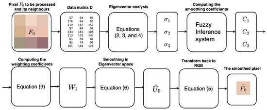
Figure 1.
Flowchart of the Gaussian denoising proposed method that outlines the processing steps applied to a single pixel.
4. Experimental Setting of the Proposed Methods, Validation and Discussion
4.1. Optimization of the Membership Functions
Parameter optimization offers a standard and reliable tool to enhance the numerical accuracy of fuzzy inference systems while maintaining their interpretability [32]. There is a plethora of techniques that address this process, with genetic algorithms (GAs) [33] demonstrating considerable success in optimizing both structure (i.e., rule definition and system architecture) and membership function parameters within each fuzzy subset.
Genetic algorithms (GAs) represent a class of global stochastic optimization methods. Their foundation lies in the principles of Darwinian survival of the fittest and natural selection (in evolutionary theory applied to animal species). This well-established approach has shown its effectiveness as an optimization technique in challenging real-world problems, particularly in the domains of design and combinatorial optimization [34].
In this context, and for each generation, a specific number of individuals is randomly created, forming the so-called initial population of candidate solutions. Subsequent generations are created through the application of variation, selection, and inheritance principles. Algorithm 1 establishes how these methodologies work.
| Algorithm 1: Genetic Algorithm |
|
In our case, a genetic algorithm (GA) is applied in order to optimize the input and output membership functions independently, for each one of the FIS methods, with the aim to enhance the noise reduction performance of Fuzzy Inference System (FIS) methods. To achieve this, we select a diverse set of three images Pills (), Headphone (), and Parrots () shown in Figure 2. These images are subjected to varying levels of Gaussian noise, . Meanwhile, the optimization process itself focuses on a single noise level at a time for the three images. In order to assess the quality of noise reduction achieved by the optimized membership functions, we employ the Peak Signal-to-Noise Ratio (PSNR) metric [4]. The key advantage of this independent optimization lies in its ability to account for the inherent differences in value ranges across various input and output variables. For example, the concept of “low” might have significantly different interpretations for each level of noise. By optimizing independently, we ensure that the membership functions adapt effectively to these diverse ranges of noise levels. The optimization process itself uses a fitness function that aims to minimize the mean squared error (MSE) between the original and denoised pixel colour values. The optimization process starts with the third channel, which typically holds the most part (the most important) information, followed by the second channel using the smoothing coefficients obtained from the optimization of the third one. Finally, the first channel is optimized using the smoothing coefficients from both the third and the second channels. This sequential approach ensures that channels with more prominent information are the guide for the noise reduction process in subsequent channels. The input membership functions in both FuzzyEIG1 and FuzzyEIG2 methods are restricted to [0–200] for both the location centre and width parameters. Output membership functions are in the [0–1] interval for both the centre and the width parameters.
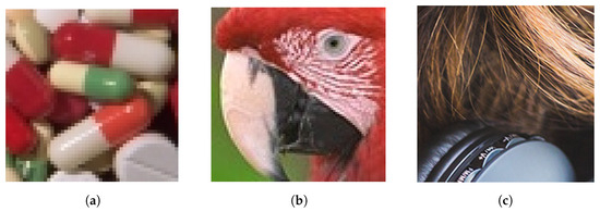
Figure 2.
Group of images selected for the training stage. (a) Pills (50 × 50); (b) Parrots (80 × 80); (c) Head-Phone (200 × 200).
The parameters corresponding to the optimized membership functions for FuzzyEIG1 and FuzzyEIG2 are shown in Table 1 and Table 2, respectively. These tables can be used as references for parameter setting when using the proposed methods.

Table 1.
Optimized parameters of the FuzzyEIG1 membership functions for the input and output stages.
Table 2.
Optimized parameters of the FuzzyEIG2 membership functions for the input and output stages.
In general, the membership function parameters change substantially across different noise levels, somehow revealing an adaptation to the noise level. The main tendency is related to membership functions increasing in overlapping as the noise increases, which reflects the adaptation that the method shows as the uncertainty in the data increases. This uncertainty is related to the location of the membership functions being closer or the width being enlarged.
This adaptive behaviour allows for the system to deal with higher standard deviation values that might be present in the data. However, the impact of noise varies across inputs, with the first input being more affected due to its association with less correlated data variations. Table 2 shows, for FuzzyEIG2, that noise also shifts the location of the output functions. This leads to higher smoothing coefficients, which is a desirable outcome for noise reduction.
4.2. Denoising Results and Discussion
Following the optimization stage, we tested the methodology by using a validation set of four images with different sizes: Beach (), Lena (), Grass (), and Micro () shown in Figure 3. These validation images, similar to the training images, were corrupted with varying levels of Gaussian levels: . To comprehensively assess the performance of our method, we employed five different metrics:
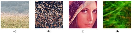
Figure 3.
Group of images selected for the validation stage. (a) Grass (200 × 200); (b) Beach (100 × 100); (c) Lenna (90 × 90); (d) Micro (51 × 51).
- Mean absolute error (MAE) [4]: It is particularly aimed at assessing detail preservation.
- Peak signal-to-noise ratio (PSNR) [4]: It measures noise cancellation.
- Normalized color difference (NCD) [4]: It evaluates colorimetric preservation.
- Fuzzy color structural similarity (FCSS) [35]: It is a color extension of the Structural Similaty measure, SSIM [36], that focuses on evaluating perceptual similarity.
- Perceptual difference inspired by iCAM (iCAMd) [37]: It measures colour changes form a perceptual point of view.
We compared the performance of our proposed approaches, FuzzyEIG1 and FuzzyEIG2, with several state-of-the-art denoising methods: the collaborative wavelet filter (CWF) [15], the eigenvector analysis method (EIG) [22], the method of Feed-forward denoising convolutional neural networks(DnCNN) [18], and the Graphs-based methods for simultaneous smoothing and sharpening (GMS3) as well as the Normalized graph-method for simultaneous smoothing and sharpening (NGMS3) [17].
All filters used a window with the authors’ recommended settings. Notably, the sharpening processes involved in and were ignored for a fair comparison. The experimental results are shown in Table 3, where the best and second-best results are highlighted in blue and red colours, respectively. Additionally, some of the method outputs are visualized in Figure 4 and Figure 5, along with squared error maps for each output.
Table 3.
MAE, PSNR, NCD , FCSS and iCAMd results for FuzzyEIG1, FuzzyEIG2, and 5 other denoising methods, on images of different sizes contaminated with varying levels of Gaussian noise (s). For each noise level and metric, the best performing method is highlighted in blue, while the second-best is highlighted in red.
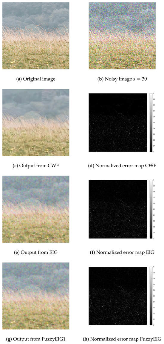
Figure 4.
Visual comparison of different denoising methods for the Grass image (). Original image (a), noisy image (b), denoised images (CWF (c), EIG (e), FuzzyEIG1 (g)), corresponding normalized squared error maps (d,f,h).
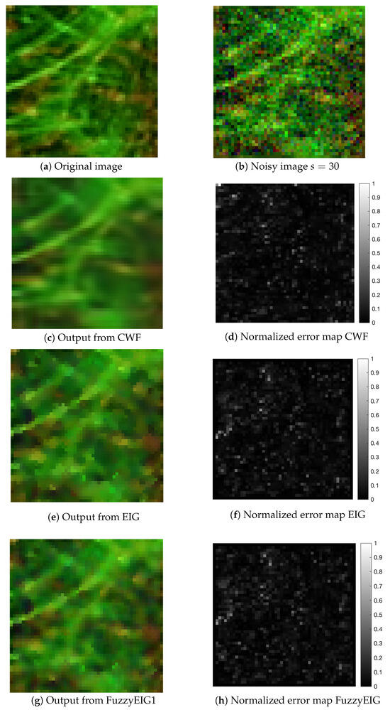
Figure 5.
Visual comparison of different denoising methods for the Micro image (). Original image (a), noisy image (b), denoised images (CWF (c), EIG (e), FuzzyEIG1 (g)), corresponding normalized squared error maps (d,f,h).
By closely examining the tables and figures, we observed that certain methods consistently outperform others across different noise levels and image sizes while others have a high variable performance. In particular, probably the highest varibility in performance was shown by the DnCNN method, which we associated to training bias. Machine learning-based denoising methods are difficult to fully understand and are biased by the training dataset used to set their parameters. Consequently, it is hard to fully trust them in any scenario. On the other hand, the other methods in the experimental comparison are interpretable. Notably, the FuzzyEIG1 and FuzzyEIG2 methods demonstrated competitive performance, often ranking among the top two performers across multiple metrics. This is primarily due to their ability to enhance the smoothing capability of the EIG method in image areas with greater homogeneity.
However, it is important to clarify that they did not outperform CWF in such areas. CWF indeed achieved the best results in homogeneous regions due to its non-local block-matching approach, which is significantly more computationally expensive. This is understandable because its block-matching approach effectively finds more matches in these areas at an expense of higher computational load. Moreover, for example, in the Lenna images with noise level , we saw a 2-unit improvement in the PSNR of the proposed methods over the EIG method. However, there were slight variations in performance for detailed images, where FuzzyEIG1 and FuzzyEIG2 lost some performance with respect to EIG but still outperformed the non-local method CWF. For instance, in the Beach image with noise level , the proposed methods achieved around a 1 unit higher PSNR than CWF while they were only below EIG. So, the benefit provided by the proposed methods is an increased performance in noise reduction with respect to EIG while keeping a good level of detail preservation although a bit lower than EIG.
Visually, in Figure 4, the CWF-processed “Grass” image exhibits some blurring in the top cloud areas compared to FuzzyEIG1 and EIG. While FuzzyEIG1 and EIG leave some noise to preserve details, CWF prioritizes smoothness, leading to this visible loss of sharpness. This trend is further evident in Figure 5. Here, the “Micro” image processed by CWF is noticeably blurred compared to FuzzyEIG1, which retains details closer to the EIG output.
A detailed analysis of the performance revealed that the limitation of the proposed methods arises during the defuzzification phase. The highest smoothing is achieved for coefficients , whereas EIG level detail preservation happens for . However, after defuzzification, values never reach the extremes of 0 or 1. This is shown in Figure 6. Here, we can see, particularly for , that higher values are associated to image edges and detail regions to be preserved but they are far from the top value of 1. Conversely, neither 0 is reached for maximum smoothing in flat regions. This results in two key trade-offs: (1) Incomplete Smoothing in Homogeneous Regions: Since C cannot reach 0, maximum noise reduction in flat areas is limited. (2) Sub-optimal Detail Preservation: this limitation prevents C from reaching 1, although it only leads to small detail loss compared to EIG. Despite this limitation, the proposed methods excel at denoising flat regions compared to EIG filtering. This is because they effectively assign low enough C values in these areas, achieving strong noise reduction while maintaining details.
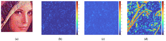
Figure 6.
Maps of the smoothing coefficients for each colour channel in the Lenna image with noise level . (a) Noisy image ; (b) C1; (c) C2; (d) C3.
This improved performance is also seen in the histogram plots presented in Figure 7 and Figure 8, where the proposed method performance lies in between CWF and EIG. These histograms plot, in the x axis, the normalized error, where the normalisation factor corresponds to the maximum error for any pixel in the denoising methods that are compared (CWF, EIG, FuzzyEIG1 and FuzzyEIG2). We only show CWF, EIG, and FuzzyEIG1 for interpretability purposes. We can see that CWF has a higher number of pixels with low error values when the image contains large homogeneous regions. This is the case, for instance, of the histograms for Grass (Figure 7). However, when there are more edges, the EIG and FuzzyEIG1 methods outperform CWF, as seen in the Beach histograms (Figure 8).
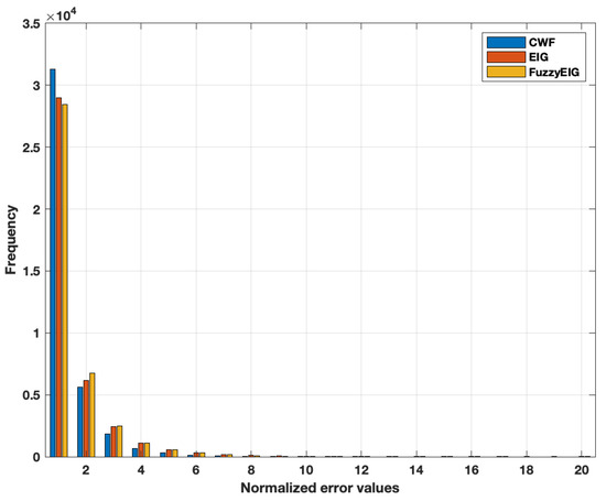
Figure 7.
The combined histogram visualizes the distributions of normalized squared error values obtained from three denoising methods applied to an image with “Grass ” noise level . The x-axis represents the range from 0 (perfect reconstruction) to 1 (maximum error), and the y-axis represents the frequency of each error value.
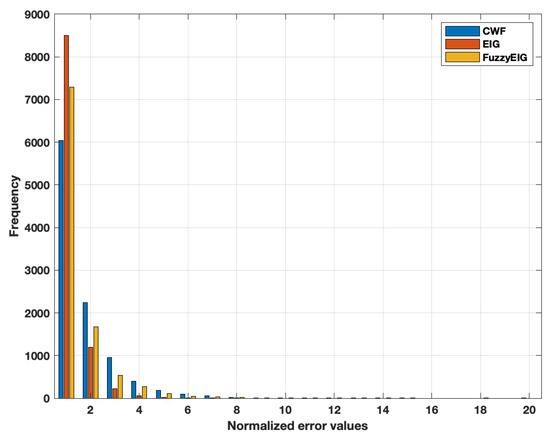
Figure 8.
The combined histogram visualizes the distributions of normalized squared error values obtained from three denoising methods applied to an image with “Beach ” noise level . The x-axis represents the range from 0 (perfect reconstruction) to 1 (maximum error), and the y-axis represents the frequency of each error value.
In general, FuzzyEIG1 stands out for its ability to achieve low error values while balancing detail preservation and noise reduction. This performance lies in its approach to the trade-off between smoothing and detail retention. CWF prioritizes smoothness, which can be ideal in specific scenarios. However, this emphasis can lead to over-smoothing and loss of fine details in other cases/images types. FuzzyEIG methods are able to balance between smoothing and detail preservation. This makes them suitable for a wider range of image types, despite limitation in the defuzzification where the smoothing coefficients never reaching 0 or 1 (indicating full or minimal smoothing). While this suggests further potential for improvement, the current balance allows for FuzzyEIG methods to preserve details better than CWF while achieving comparable or better denoising in homogeneous regions. This balanced approach makes FuzzyEIG methods competitive across various metrics, even if they may not always surpass CWF in strictly homogeneous regions.
5. Conclusions and Future Work
Two novel image-denoising methods, FuzzyEIG1 and FuzzyEIG2, are presented in this paper, both of them based on an previous eigenvector-based strategy, EIG. While both methods achieve promising results in terms of noise reduction and detail preservation, their limitations are identified. FuzzyEIG1 and FuzzyEIG2 show competitive performance across various metrics and present a more scalable behaviour. Their main advantage is an increased performance in noise reduction with respect to EIG while keeping a good level of detail preservation although a bit lower than that of EIG.
However, the methods’ performance in both noise smoothing and detail preservation is not optimal. This happens because of the defuzzification process being unable to provide values close enough to one when higher detail preservation is needed or to zero when more smoothing is appropriate.
One promising avenue for future research is the integration of neural networks (NNs) for this defuzzification (last) stage. NNs can be trained to learn the optimal parameters for the defuzzification process, potentially improving both efficiency and accuracy. This hybrid approach would combine the strengths of both methods, leveraging the data-driven learning capabilities of NNs with the adaptability of FuzzyEIG methods. Ultimately, continuous exploration and refinement are crucial for developing robust and adaptable image-denoising techniques suitable for real-world applications.
Author Contributions
Conceptualization, K.A., S.M. and P.L.-C.; methodology, K.A, S.M. and P.L.-C.; software, K.A.; validation, K.A., S.M. and P.L.-C.; formal analysis, K.A., S.M. and P.L.-C.; investigation, K.A., S.M. and P.L.-C.; resources, S.M.; data curation, K.A., S.M. and P.L.-C.; writing—original draft preparation, K.A., S.M. and P.L.-C.; visualization, K.A., S.M. and P.L.-C.; supervision, S.M. and P.L.-C.; project administration, S.M.; funding acquisition, S.M. All authors have read and agreed to the published version of the manuscript.
Funding
This research was funded by Generalitat Valenciana under grant CIAICO/2022-051 IMaLeVICS and Spanish Ministry of Science under grant PID2022-140189OB-C21.
Data Availability Statement
The data and the code will be available upon a reasonable request.
Conflicts of Interest
The authors declare no conflicts of interest.
References
- Liu, W.; Lin, W. Additive white Gaussian noise level estimation in SVD domain for images. IEEE Trans. Image Process. 2013, 22, 872–883. [Google Scholar] [CrossRef] [PubMed]
- Swenson, G.W.; Thompson, A.R. Radio Noise and Interference. In Reference Data for Engineers, 9th ed.; Middleton, W.M., Van Valkenburg, M.E., Eds.; Newnes: Oxford, UK, 2020; pp. 34-1–34-13. [Google Scholar] [CrossRef]
- Price, J.; Goble, T. Signals and Noise. In Telecommunications Engineer’s Reference Book; Mazda, F., Ed.; Butterworth-Heinemann: Oxford, UK, 1993; pp. 10-1–10-15. [Google Scholar] [CrossRef]
- Plataniotis, K.N.; Venetsanopoulos, A.N. Color Image Processing and Applications; Springer: Berlin/Heidelberg, Germany, 2000. [Google Scholar]
- Lukac, R.; Smolka, B.; Martin, K.; Plataniotis, K.N.; Venetsanopoulos, A.N. Vector Filtering for Color Imaging. IEEE Signal Process. Mag. 2005, 22, 74–86. [Google Scholar] [CrossRef]
- Lukac, R.; Plataniotis, K.N. A Taxonomy of Color Image Filtering and Enhancement Solutions. In Advances in Imaging and Electron Physics; Hawkes, P.W., Ed.; Elsevier Academic Press: Amsterdam, The Netherlands, 2006; Volume 140, pp. 187–264. [Google Scholar]
- Buades, A.; Coll, B.; Morel, J.M. Nonlocal Image and Movie Denoising. Int. J. Comput. Vision 2008, 76, 123–139. [Google Scholar] [CrossRef]
- Tomasi, C.; Manduchi, R. Bilateral filter for gray and color images. In Proceedings of the IEEE International Conference Computer Vision, Bombay, India, 4–7 January 1998; pp. 839–846. [Google Scholar]
- Elad, M. On the origin of bilateral filter and ways to improve it. IEEE Trans. Image Process. 2002, 11, 1141–1151. [Google Scholar] [CrossRef]
- Kao, W.C.; Chen, Y.J. Multistage Bilateral Noise Filtering and Edge Detection for Color Image Enhancement. IEEE Trans. Consum. Electron. 2005, 51, 1346–1351. [Google Scholar]
- Garnett, R.; Huegerich, T.; Chui, C.; He, W. A Universal Noise Removal Algorithm with an Impulse Detector. IEEE Trans. Image Process. 2005, 14, 1747–1754. [Google Scholar] [CrossRef]
- Morillas, S.; Gregori, V.; Sapena, A.F. Fuzzy Bilateral Filtering for Color Images. Lect. Notes Comput. Sci. 2006, 4141, 138–145. [Google Scholar]
- Mehra, M.; Mehra, V.K.; Ahmad, M. Wavelets Theory and Its Applications; Springer: Singapore, 2018. [Google Scholar]
- Dabov, K.; Foi, A.; Katkovnik, V.; Egiazarian, K. Image Denoising by Sparse 3D Transform-Domain Collaborative Filtering. IEEE Trans. Image Process. 2007, 16, 2080–2095. [Google Scholar] [CrossRef]
- Dabov, K.; Foi, A.; Katkovnik, V.; Egiazarian, K. Color Image Denoising via Sparse 3D Collaborative Filtering with Grouping Constraint in Luminance-Chrominance Space. In Proceedings of the IEEE International Conference on Image Processing (ICIP 2007), San Antonio, TX, USA, 16–19 September 2007; pp. 313–316. [Google Scholar]
- Hao, B.B.; Li, M.; Feng, X.C. Wavelet Iterative Regularization for Image Restoration with Varying Scale Parameter. Signal Process. Image Commun. 2008, 23, 433–441. [Google Scholar] [CrossRef]
- Pérez-Benito, C.; Jordán, C.; Conejero, J.A.; Morillas, S. Graphs-based methods for simultaneous smoothing and sharpening. MethodsX 2020, 7, 100819. [Google Scholar] [CrossRef] [PubMed]
- Zhang, K.; Zuo, W.; Chen, Y.; Meng, D.; Zhang, L. Beyond a gaussian denoiser: Residual learning of deep cnn for image denoising. IEEE Trans. Image Process. 2017, 26, 3142–3155. [Google Scholar] [CrossRef]
- Oja, E. Principal components, minor components, and linear neural networks. Neural Netw. 1992, 5, 927–935. [Google Scholar] [CrossRef]
- Takahashi, T.; Kurita, T. Robust de-noising by kernel PCA. In Proceedings of the ICANN2002, Lecture Notes in Computer Science, Madrid, Spain, 28–30 August 2002; Volume 2145, pp. 739–744. [Google Scholar]
- Park, H.; Moon, Y.S. Automatic Denoising of 2D Color Face Images using Recursive PCA Reconstruction. In Proceedings of the Advanced Concepts for Intelligent Vision Systems ACIVS06, Lecture Notes in Computer Science, Antwerp, Belgium, 18–21 September 2006; Volume 4179, pp. 799–809. [Google Scholar]
- Latorre-Carmona, P.; Miñana, J.-J.; Morillas, S. Colour Image Denoising by Eigenvector Analysis of Neighbourhood Colour Samples. Signal Image Video Process. 2020, 14, 483–490. [Google Scholar] [CrossRef]
- Zadeh, L.A. Fuzzy Sets. Inf. Control 1965, 8, 338–353. [Google Scholar] [CrossRef]
- Sabri, N.; Aljunid, S.A.; Salim, M.S.; Badlishah, R.B.; Kamaruddin, R.; Malek, M.A. Fuzzy Inference System: Short Review and Design. Int. Rev. Autom. Control 2013, 6, 441–449. [Google Scholar]
- Schulte, S.; De Witte, V.; Kerre, E.E. A Fuzzy Noise Reduction Method for Color Images. IEEE Trans. Image Process. 2007, 16, 1425–1436. [Google Scholar] [CrossRef]
- Schulte, S.; Witte, V.D.; Nachtegael, M.; M’elange, T.; Kerre, E.E. A New Fuzzy Additive Noise Reduction Method. In Proceedings of the International Conference Image Analysis and Recognition, Montreal, QC, Canada, 22–24 August 2007; pp. 12–23. [Google Scholar]
- Van De Ville, D.; Nachtegael, M.; Van der Weken, D.; Kerre, E.E.; Philips, W.; Lemahieu, I. Noise Reduction by Fuzzy Image Filtering. IEEE Trans. Fuzzy Syst. 2003, 11, 429–436. [Google Scholar] [CrossRef]
- Almutairi, K.; Morillas, S.; Latorre-Carmona, P. Fuzzy Inference System in a Local Eigenvector Based Color Image Smoothing Framework; Scitepress: Prague, Czech Republic, 2023. [Google Scholar]
- Dillon, W.R.; Goldstein, M. Multivariate Analysis: Methods and Applications; Wiley: Hoboken, NJ, USA, 1984. [Google Scholar]
- Jackson, J.E. A User’s Guide to Principal Components; Wiley: Hoboken, NJ, USA, 2003. [Google Scholar]
- Mendel, J.M. Fuzzy Logic Systems for Engineering: A Tutorial. Proc. IEEE 1995, 83, 345–377. [Google Scholar] [CrossRef]
- Casillas, J.; Cord’on, O.; Herrera, F.; Magdalena, L. Interpretability Improvements to Find the Balance Interpretability-Accuracy in Fuzzy Modeling: An Overview. In Interpretability Issues in Fuzzy Modeling; Springer: Berlin/Heidelberg, Germany, 2003; pp. 3–22. [Google Scholar]
- Moallem, P.; Mousavi, B.; Naghibzadeh, S.S. Fuzzy Inference System Optimized by Genetic Algorithm for Robust Face and Pose Detection. Int. J. Artif. Intell. 2015, 13, 73–88. [Google Scholar]
- Abualigah, L.M.Q.; Hanandeh, E.S. Applying genetic algorithms to information retrieval using vector space model. Int. J. Comp. Sci. Eng. Appl. (IJCSEA) 2015, 5, 19–28. [Google Scholar] [CrossRef]
- Grecova, S.; Morillas, S. Perceptual similarity between color images using fuzzy metrics. J. Visual Commun. Image Represent. 2016, 34, 230–235. [Google Scholar] [CrossRef]
- Wang, Z.; Bovik, A.C.; Sheikh, H.R.; Simoncelli, E.P. Image quality assessment: From error visibility to structural similarity. IEEE Trans. Image Process. 2004, 13, 600–612. [Google Scholar] [CrossRef] [PubMed]
- Fairchild, M.D.; Johnson, G.M. ICAM Framework for Image Appearance, Differences, and Quality. J. Electron. Imaging 2004, 13, 126–138. [Google Scholar] [CrossRef]
Disclaimer/Publisher’s Note: The statements, opinions and data contained in all publications are solely those of the individual author(s) and contributor(s) and not of MDPI and/or the editor(s). MDPI and/or the editor(s) disclaim responsibility for any injury to people or property resulting from any ideas, methods, instructions or products referred to in the content. |
© 2024 by the authors. Licensee MDPI, Basel, Switzerland. This article is an open access article distributed under the terms and conditions of the Creative Commons Attribution (CC BY) license (https://creativecommons.org/licenses/by/4.0/).