Abstract
This work proposes an analytical design procedure for a particular class of 2D filters, namely anisotropic Gaussian FIR filters. The design is achieved in the frequency domain and starts from a low-pass Gaussian 1D prototype with imposed specifications, whose frequency response is efficiently approximated by a factored trigonometric polynomial using the Chebyshev series. Then, using specific 1D to 2D frequency mappings applied to the prototype, the frequency response for a 2D anisotropic filter with a specified orientation angle is directly derived in two versions, namely with a straight or elliptical shape in the frequency plane. The resulting filters have an accurate shape with low distortion. Several design examples for specified parameters (angle and selectivity) are provided. Then, simulations of directional filtering on various test images are given, which show their capability of extracting oriented lines or other various oriented objects from synthetic or real-life images. Finally, a computationally efficient implementation at the system level is proposed, based on a polyphase decomposition and block-filtering approach, which yields a 2D filter with a high degree of parallelism and low arithmetic complexity.
1. Introduction
Ever since the emergence of 2D filters within the broader field of digital signal and image processing, the analytic design techniques for these filters have become a valuable alternative approach as compared to the more traditional numerical optimization algorithms, which usually lead to optimal filters for a set of imposed specifications. The analytical methods rely on various specific frequency transformations that are applied to a convenient 1D prototype filter with imposed parameters, thus directly obtaining the frequency response of the desired 2D filter [1,2,3,4].
Depending on their application, 2D filters (both the FIR and IIR type) may have frequency characteristics of various shapes, for instance, circular, elliptically shaped, square, fan, etc. A particular class is the orientation-selective or directional 2D filters used in fundamental image processing tasks such as edge detection, texture analysis, segmentation, optical flow estimation, etc.
Gaussian-shaped filters form a special class of 2D filters, currently employed in important tasks such as image smoothing through the blurring effect, achieved by a local averaging of pixels within a specified radius. Such Gaussian 2D filters most often have circular support but may also have an anisotropic shape in the frequency plane, thus achieving directional filtering. Several design procedures and efficient implementations of directional Gaussian filters, some of them including decomposition of the frequency response along two or three axes, are proposed in early or more recent papers such as [5,6,7,8]. Such anisotropic Gaussian filters find applications like directional smoothing, in particular for enhancing or restoring remote sensing images [9,10], and they are also useful in edge detection [11]—especially in noisy images [12]—or in optical flow estimation [13]. Multiresolution directional filter banks, their design methods, and their applications are treated in this comprehensive work [14].
Some very recent papers have approached various advanced design techniques for 2D FIR and IIR filters [15,16,17,18,19,20]. A low-complexity 2D FIR filter implementation based on a Farrow structure is proposed in [21]. Various soft computing design algorithms have also been developed, like the Lévy flight firefly algorithm [22] or the Vortex Search algorithm [23]. New implementations and applications of 2D Gabor filters are given in [24,25], while a low-cost 2D median filter is approached in [26]. Advanced applications are proposed for SAR imaging [27], the denoising of satellite images [28], and SAR interferograms [29], while directional filters are used in sonar image fusion [30]. Other recent developments include a neural Fourier filter bank [31], continuous upsampling filters [32], 2D matched filtering with time-stretching [33], 2D/3D convolution techniques for hyperspectral image super-resolution [34], and two-dimensional polynomial predictors [35]. Hardware-efficient multiplier-less structures are proposed in [36,37]. Minimal state-space realizations, including lattice structures, are proposed in [38,39], while high-performance architectures on FPGA are developed in [40,41]. Area-efficient 2D structures for 2D filtering are also approached in [42,43]. A computational complexity evaluation of 2D filtering by the Winograd method is performed in [44]. Novel stability tests for 2D continuous-time systems are established in [45].
A rather difficult issue in fields such as computer vision and object and scene recognition is the problem of straight-line detection. A widely used method for detecting lines is based on the Hough transform (HT), a computationally intensive algorithm using edge detection and then the mapping of edge points onto the so-called Hough space. A regularized HT capable of detecting straight lines in grayscale images is developed in [46]. An improved version of the HT algorithm relies on the Freeman chain code [47], significantly diminishing computation time as compared to the standard HT. A high-performance 2D parallel block-filtering system developed for real-time applications is described in [48].
Various analytic techniques for the design of 2D filters, in particular with directional characteristics, have been proposed by the first author in previous papers, such as parametric IIR filters for directional Gaussian smoothing [49]; directional and square-shaped 2D IIR filters based on digital prototypes [50,51]; directional Gaussian 2D FIR filters, separable along three axes [52]; and adjustable 2D filters with elliptical and circular symmetry [53]. A computationally efficient implementation for a 2D circular FIR filter bank, based on a polyphase decomposition approach, has been proposed in [54].
This work proposes an analytical procedure for the design of a particular class of 2D filters, namely directional Gaussian FIR filters with specified selectivity and orientation of the frequency response. Two such filter types are presented, one with a straight shape and the other with an elliptical shape of the frequency response support in the frequency plane. For each type, a specific 1D to 2D frequency transformation is derived and then applied to the suitable prototype. The filters are parametric, and their kernels result as being directly decomposed as a convolution of smaller-size matrices. To demonstrate their capabilities in image processing applications, several directional filtering simulations are provided on various test images. A parallel implementation technique for these filters is also shown, using polyphase decomposition and block filtering; this method is computationally efficient, requiring a relatively small number of arithmetic operations.
This paper has the following structure: Section 2 presents the 1D Gaussian filter used as a prototype in design, derived through an efficient Chebyshev series approximation. The proposed analytical design method for 2D directional filters is detailed in the main section, Section 3, for the design of two distinct directional filters, namely with a straight shape or elliptical shape characteristic in the frequency plane, and several design examples are presented for the given specifications. Next, in Section 4, several simulation results of directional filtering with imposed orientation are given on various test images, highlighting their applications in image processing. A novel implementation structure relying on a polyphase approach and block-filtering technique is described in Section 5. A comparative discussion regarding the main design issues and the arithmetic complexity of the proposed implementation is made in Section 6. The conclusion paragraph summarizes the main aspects of the paper and sets objectives for further work.
2. Outline of the 2D Directional Filter Analytical Design Method
2.1. Motivation of the Proposed Design Approach
The proposed analytical technique adopted for the design of 2D directional filters is a precise and efficient alternative to the more traditional design method based on global numerical optimization algorithms. As shown further, the design starts from a convenient 1D prototype of a desired shape (in our case, Gaussian) and imposed specifications (order, bandwidth, selectivity, ripple, etc.); applying to the factored frequency response of this prototype a specific 1D to 2D frequency mapping, the frequency response of the corresponding 2D filter is derived directly in a factored form, which is very important in 2D design, including implementation. It is well known that, in general, a 2D function cannot be factored; this is a major drawback of currently used numerical optimization algorithms. Instead, obtaining the frequency response already factored (as in our method) is a major advantage that justifies this approach. Correspondingly, the overall filter kernel will result in being directly decomposed as a convolution of smaller-size matrices (for instance, 5 × 5), thus simplifying implementation. To the best of our knowledge, this method was not applied in other works on this topic. Another drawback of previous optimization methods is that the design process has to be redone from the start for each set of specifications. By comparison, our analytical technique is more versatile and flexible, leading to parametric filters, in which the specifications (bandwidth, selectivity, orientation angle) appear explicitly as parameters in the filter kernel. Thus, the generic 2D filter can be simply tuned or adjusted directly by simply substituting the given specifications.
Moreover, by applying the 1D–2D frequency mapping, the 2D filter will preserve the properties of the prototype; thus, its shape can be precisely controlled. Another choice made in our design is using the very accurate and efficient Chebyshev–Padé approximation, which leads to 2D filters with a precise shape, negligible distortions, and a relatively low order for their high selectivity. Finally, the proposed filter implementation based on polyphase and block filtering ensures a high degree of parallelism with a very low computational complexity.
2.2. 1D Gaussian Prototype Filters
In order to obtain directional 2D filters through the proposed analytical procedure, we need to start with a convenient low-pass 1D prototype filter. Although several such prototypes may be chosen for efficient 2D directional filters, a very selective prototype with a narrow characteristic would be required. One very appropriate choice that suits our purpose would be a Gaussian filter, which can be easily approximated and efficiently implemented. Being described by a real transfer function, which is also its frequency response, it has a very useful zero-phase property; for this reason, it is widely used in image processing applications, as it does not cause any phase distortions in the filtered image. Let us consider the following simple 1D prototype given by a Gaussian function in the frequency domain, where is the dispersion parameter:
In order to simplify the following calculations, at this point, we introduce the so-called selectivity parameter , and thus, the Gaussian (1) is expressed equivalently as ; for larger values of p, the Gaussian prototype will be more selective [49,52]. In order to finally obtain the frequency response of a 2D discrete filter, we need to efficiently approximate this Gaussian prototype. For the proposed method, the most convenient approach is the Chebyshev series, which yields a very efficient, uniform approximation of a given function over a specified interval, ensuring an optimal tradeoff between precision and the order of complexity. Its only drawback, unlike the Taylor series, is that its coefficients are only determined numerically, for instance, using a symbolic computation software like MAPLE 2018. Since the 1D prototype generates a directional filter with a specified orientation angle, the approximation must be valid on a range larger than , at least , which allows to avoid any marginal distortions of the 2D filter towards frequency plane corners, where the approximation may diverge.
Since our approximation must yield a trigonometric polynomial in , before applying the Chebyshev series, the following change in the variable is introduced [50,51]:
Applying the substitution (2), first, we find the Chebyshev series of the intermediate function , with an imposed error of 0.04:
Replacing back in {3) x by , the following approximation is derived as a polynomial in the variable , which in factored form is given by:
The above prototype of low order will be used to design 2D directional filters with an elliptically shaped frequency response in Section 3.4.
For Gaussian filters with higher selectivity, obtained for larger values of parameter p, the Chebyshev series must be truncated at a higher order, preserving more terms in order to obtain a good approximation with the imposed accuracy. For instance, specifying a parameter p = 25, the following trigonometric approximation was derived:
This more selective prototype will be further used to derive a narrow, straight directional filter with a specified orientation, in Section 3.3. The two Gaussian-shaped prototypes given by (4) and (5) are displayed in Figure 1a and Figure 1b, respectively. The approximations for and were calculated with the precision . Both prototypes have precise frequency responses with negligible distortions. The prototype has a very low ripple in the stopband.
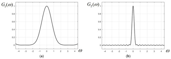
Figure 1.
Plot of Gaussian approximations: (a) and (b) .
3. Analytical Design Procedure for Anisotropic 2D FIR Filters
This main section presents in detail the proposed analytical design technique for two types of anisotropic FIR filters, namely with straight-shaped and elliptically shaped frequency responses, respectively.
3.1. Frequency Transformations for Anisotropic 2D FIR Filters
In this work, two different types of directional filters are approached. Both versions are derived analytically by applying two different 1D to 2D frequency mappings to the factored transfer function of a 1D low-pass prototype with a specified selectivity. The two types of anisotropic filters designed here have a Gaussian shape in a vertical section along their longitudinal symmetry axes. However, their shapes differ in a horizontal section, as the corresponding contour plots will show. For the first filter type, the frequency response has a straight shape, while for the second filter, it has an elliptical shape. The design steps for the two filter types will be presented in the following sections.
3.1.1. Frequency Transformation for Straight Anisotropic Filters
Starting from a specified 1D prototype , a 2D directional filter results by rotating the axes of the frequency plane with a given angle about axis. This rotation is described by the 1D to 2D frequency transformation [50,51]:
Applying this frequency mapping by simple substitution into the Gaussian prototype , the following 2D frequency response results, where the subscript D means directional:
3.1.2. Frequency Transformation for Elliptically Shaped Anisotropic Filters
The second type of directional filters presented here are filters with elliptically shaped support in the frequency plane. These filters are specified by the major and minor semi-axes of the ellipse (E, F), while the orientation is given by the angle of the major axis with respect to the axis. Starting from the same Gaussian prototype , a directional filter with elliptically shaped support results by applying the following frequency transformation , with the following expression [53]:
where the coefficients , , and are found by direct identification. In the mapping (8), E and F are the values of the major and minor semi-axes of the ellipse. Through this analytical approach, based on the Gaussian prototype (4), we derived a 2D filter with elliptical support, described by parameters E, F, and , which define the shape and orientation through mapping (8).
3.2. Examples of Ideal Gaussian Anisotropic Filters
Prior to introducing the analytical design method, two ideal anisotropic filters are discussed, with straight and elliptical-shaped frequency responses, respectively.
Example 1.
Let us consider a straight anisotropic filter with orientation angle , derived from the Gaussian prototype . Using the mapping (6), the following ideal 2D frequency response is obtained:
This ideal straight frequency response is displayed in Figure 2a, and its contour plot is in Figure 2b. The ideal directional filter has a transversal section along the line identical to the prototype , and is constant (equal to 1) along the line (the filter longitudinal axis).
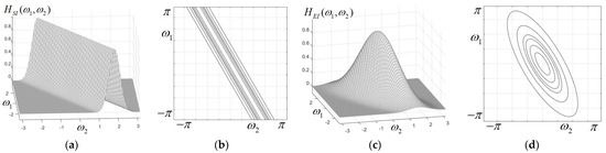
Figure 2.
Frequency response (a) and contour plot (b) for an ideal straight anisotropic filter with ; frequency response (c) and contour plot (d) for a Gaussian elliptically shaped anisotropic filter with E = 3.6, F = 0.9, and .
Example 2.
Let us consider an elliptical directional filter with an orientation angle of and the ellipse semi-axes and . Then, mapping (8) yields the elliptical directional frequency response:
3.3. Design of Anisotropic 2D FIR Filters with Straight Longitudinal Shape
Taking into account the 1D to 2D frequency mapping (6), the following design step is to make a simple substitution in each factor of the prototype function, as below:
The function will be referred to as the ideal oriented cosine function in the frequency variables , . Further, we need to find an approximation of the ideal function , expressed in and , which can be directly implemented as a 2D discrete filter.
Next, a low-order efficient 1D to 2D frequency mapping will be obtained. Applying this mapping to the Gaussian prototype will lead directly to the desired 2D directional filter. In this paper, we use two approximations, namely the Taylor and the Chebyshev series approximations. Even if the Taylor approximation only holds within a limited vicinity of the current point—while the Chebyshev series gives a uniform approximation with a constant error on a given range—for the first type of very selective directional filter, with a straight longitudinal shape of the frequency response, the Taylor approximation is more suitable, yielding directional filters with less shape distortions, as the following design examples will show.
Thus, we use the Taylor approximation of minimum order for :
Next, we look for a low-order approximation of as a trigonometric polynomial in . Since we do not need a precise, uniform approximation on the entire range , but mainly around zero, we will again use the Taylor series, as above. However, the variable change is first applied. In this way, we derive the Taylor series of around the point , truncated to the second-order term:
Now, replacing back in (13) and applying the usual trigonometric identities, we reach the second-order approximation:
As can be remarked, this approximation (which is plotted as curve 2 in Figure 3a) is accurate around zero, diverging significantly from the approximated function (curve 1) towards the margins of the interval . Applying the mapping (6), we just have to substitute with the expression:
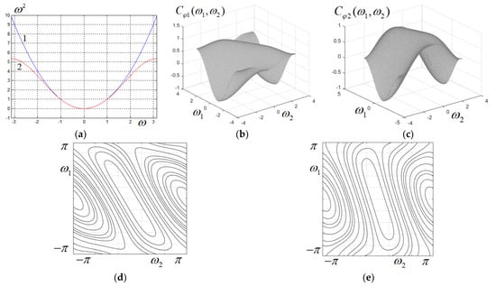
Figure 3.
(a) Function (in blue) and its approximation (in red) using Taylor series; oriented cosine function for orientation angles: (b) and (c) . (d,e) Contour plots corresponding to characteristics (b) and (c), respectively.
Using the identity and expressing the coefficients resulting from (15) leads to the following mapping:
where the coefficients a, b, and c are identified as the following:
The trigonometric approximation (14) can be written separately for the frequency variables , and their sum , obtaining the following set of approximations:
Replacing the expressions (18) into (16) and then into (12), the is mapped into a trigonometric polynomial expressed in the variables and , which may be regarded as a discrete space Fourier transform; through a direct identification of coefficients, it is easy to show that the function corresponds to the centrally symmetric matrix
whose elements have the following expressions depending on the orientation angle , as follows:
As an example, for , we obtain from (19) the following matrix:
This corresponds to the oriented cosine function shown in Figure 3b.
Thus, through these successive approximations and substitutions, we have derived an approximation of the ideal mapping (11), namely:
where is the 2D DFT (discrete Fourier transform) of the matrix , determined as shown before.
In Figure 3b–e, the function and its corresponding contours are shown for two orientation angles, namely and . It is visible, mainly from the contours, that the characteristics have a straight linear shape in their central longitudinal portion, which is essential for designing very selective directional filters.
According to the approximations (4) and (5), the prototype frequency response can be factored into first- and second-order polynomials in the variable :
where k is a constant and is the filter order. Making the substitution (22) directly in all factors of from (23), the following factored 2D directional frequency response results as follows:
where C is a short notation for . Because the specified prototype filter is already factored, the directional filter obtained by frequency mapping will also result in a factored transfer function. Corresponding to the factored transfer function in (24), the kernel of the FIR filter, although being of large size, already results as directly decomposed into smaller-size matrices (size or ), and the symbol represents the operation of the matrix convolution:
The FIR filter kernel corresponds to the transfer Function (24). Taking into account (24), each matrix (of size ) from (25) is derived from by adding the value from each factor in (24) to the central element of matrix . The larger matrices (of size ) correspond to the second-order factors from (23), and thus we have the following expression:
In the expression (26), is a null matrix, with the central element being one; the matrix results by padding () with zeros up to the size .
Following the procedure described before, three very selective directional filters with straight frequency responses derived from the narrow prototype (5) are given as the design examples in Figure 4 for the specified orientation angle . It can be noticed they have accurate characteristics with negligible distortions (a small ripple in the stopband region). The contours also indicate a good longitudinal linearity, a perfectly straight shape, and no other visible distortions.
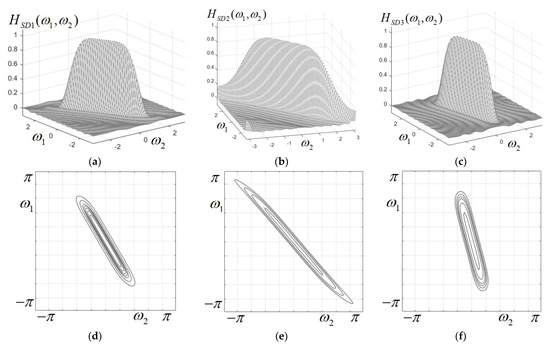
Figure 4.
Frequency responses for directional Gaussian filters with orientation angles: (a) , (b) , and (c) ; (d), (e), (f) contour plots for these filters, respectively.
3.4. Design of Anisotropic 2D FIR Filters with Elliptical Longitudinal Shape
According to Section 3.1.2, starting from the chosen Gaussian prototype, a 2D elliptically shaped filter is derived, with the parameters E, F, and . Using the simple identity , the mapping (8) takes the following form:
Using the notations , , the coefficients a, b, and c will have the following expressions:
Applying the mapping (27) to the Gaussian prototype , the 2D frequency response results (where the subscript E denotes elliptical) as follows:
Since the Gaussian 1D prototype with a specified selectivity is expressed as a factored trigonometric polynomial in the variable , we will need the following frequency mapping derived from (27):
In order to find a convenient expression for this frequency mapping, we will use the efficient Chebyshev series approximation, which is known to yield an accurate and uniform approximation of a given function on a specified interval. Thus, we obtain the following very accurate approximation (for , specifically ):
Taking into account Equation (30), we immediately obtain:
On the other hand, again using the Chebyshev series method and variable change (2), we obtain the following trigonometric approximation for the function :
This can be written separately for the frequency variables , and their sum , obtaining the set of approximations:
Substituting relations (34) into (27) and then the obtained expression of into (32), we obtain a trigonometric expression of in the variables and . Regarding this expression as a 2D discrete Fourier transform, by a simple identification of the coefficients, we finally obtain a matrix of the general centrally symmetric form, similar to from (19):
where this time, the matrix elements have the following expressions depending on the ellipse aspect parameters p, q, and on the orientation angle :
Since the derived matrix corresponds to the expression , then according to Equation (32), the function will correspond to a matrix given by the following expression:
where the symbol represents the operation of matrix convolution.
In the expression above, is a null matrix, with the central element being one; the matrix results by bordering () with zeros up to a size of .
In Figure 5, the function and its contours are shown for several values of semi-axes and orientation angles, as specified. It is visible, mainly from the contours, that the characteristics have a correct elliptical shape, at least in their central portion, which will lead to elliptical directional filters with negligible distortions, as shown further.
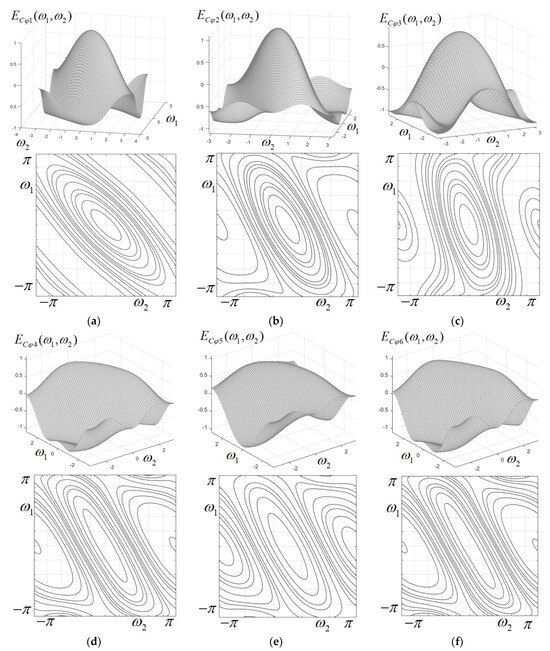
Figure 5.
Frequency responses and contour plots of the elliptical cosine function for the specified values E and F of the semi-axes and the orientation angle : (a) E = 3, F = 1, ; (b) E = 3, F = 1, ; (c) E = 3, F = 1, ; (d) E = 6, F = 1, ; (e) E = 6, F = 1.5, ; and (f) E = 8, F = 1, .
Following the above procedure, several directional filters with elliptically shaped characteristics are designed as examples; their frequency responses (for ) and the corresponding contour plots are displayed in Figure 6 for the specified parameters (semi-axes E and F and the orientation angle ).
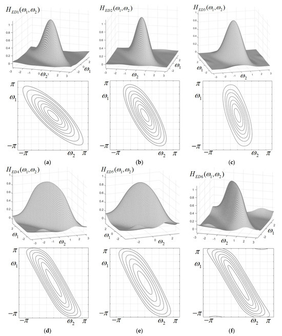
Figure 6.
Frequency responses and contour plots of some elliptically shaped directional filters for the specified values E and F of the semi-axes and the orientation angle : (a) E = 3, F = 1, ; (b) E = 3, F = 1, ; (c) E = 3, F = 1, ; (d) E = 6, F = 1, ; (e) E = 6, F = 1.5, ; and (f) E = 8, F = 1, .
As can be noticed, the characteristics have accurate shapes with negligible distortions. The contour plots also show almost perfect elliptical shapes, with minimal distortions near the margins of the frequency plane, for filters with a large aspect ratio (E/F = 8, etc.). As a remark, elliptically shaped filters with a large aspect ratio (a ratio between semi-axes values, E/F), for instance, the filter with E = 8 and F = 1 in Figure 6f, have a shape almost similar to a straight filter (the ellipse being very elongated).
As a remark, the mappings (6) and (8) can be generally applied to any prototype of a specified shape (for instance, wider and maximally flat), not necessarily Gaussian.
As another important observation, the proposed 2D anisotropic filters have to be designed only for angles between values 0 and pi/4 (within half a quadrant); for any other angle, the filter is simply obtained, taking into account the symmetry. Thus, for the specified angles outside the mentioned quadrant, the filter kernel is simply obtained by simple symmetry operations, like a rotation by 90 degrees or flipping the matrix upside-down or from left to right. A more detailed explanation of this issue is provided in [52] for another type of directional filter.
4. Applications and Simulation Results
This section will provide several relevant examples of specific applications for the anisotropic filters designed using the proposed analytical procedure. As the simulations will show, directional filters with specified orientation and selectivity are able to detect and extract straight lines and various oriented objects or details from a given image.
4.1. Examples of Directional Filtering on Various Test Images
The directional filter designed in Section 3.3 for specified orientation angles is applied on several test images, and the results are shown and discussed as follows.
The effect of directional filtering is first tested on a synthetic binary image of size pixels, shown in Figure 7a, which contains straight lines with an orientation varying gradually in the range of a quadrant. As known, the FFT spectrum of a straight line from an image also has the shape of a straight line in the frequency plane , passing through zero, and is perpendicular to the line direction. This can be obviously noticed in the logarithmic FFT spectrum magnitude (b) of image (a); it consists of a beam of thin straight lines spanning two opposite quadrants. Thus, the directional filtering is easy to understand. For a specified orientation angle, only the lines whose spectra overlap longitudinally with the narrow filter frequency response will be preserved identically in the output image, while the lines with other orientations will be blurred. Lines having the spectrum orthogonal to the filter axis will be practically erased due to blurring.
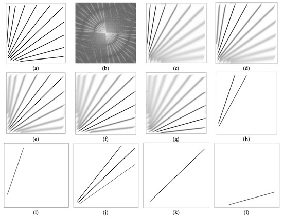
Figure 7.
(a) Binary test image “Lines”; (b) its logarithmic FFT spectrum magnitude; (c–f) directionally filtered output images for orientation angles: (c) , (d) , (e) , (f) , and (g) ; (h–l) binary images showing straight lines oriented at various angles, extracted by applying a given threshold to the previous directionally filtered images. The image and threshold value th is specified as follows: (h) image, (d) th = 0.69; (i) image, (d) th = 0.91; (j) image, (e) th = 0.66; (k) image, (e) th = 0.91; and (l) image, (g) th = 0.91.
Applying a narrow straight directional filter, the output filtered images are shown in Figure 7c–g for the indicated orientation angles. The filter preserves one or a few lines corresponding to its orientation while the other lines are gradually blurred. This directional filtering can be followed by a thresholding operation in order to detect and extract those lines, as shown in Figure 7h–l, for the indicated threshold values (considered subunitary). Prior to applying a given threshold, the pixel values of the filtered images were normalized, i.e., rescaled to the range [0, 1] (with the value 0 corresponding to black and 1 to white). Thus, directional filtering may be a pre-processing step in the application of object detection and extraction from a given image.
The second filtering simulation is run on the test image displayed in Figure 8a, which is a real grayscale texture image of pixels that represents randomly oriented straws. Applying directional filtering to image (a), with orientation angles ,, and , respectively, the resulting filtered images are (b), (c), and (d). As can be noticed, only the straws roughly matching a given orientation remain visible in the output image, while those with other orientations will be more or less blurred. The displayed output images demonstrate a good directional resolution of these filters.
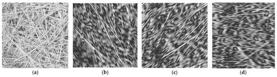
Figure 8.
(a) Straw texture image; filtered output images for (b) , (c) , and (d) .
In the third directional filtering example, the grayscale test image “Oats” contains natural objects, namely oat seeds (grains), which form a specific texture image. The oat seeds are oriented randomly under various angles. Due to their elongated shape, they can be separated through directional filtering, as shown in Figure 9. The output images for the indicated orientation angles are displayed in Figure 9b–h. The filtering effect is clearly visible. The grains whose spectrum is oriented along the filter longitudinal axis are clearly preserved in the output image, while the others are more or less blurred, depending on their orientation.
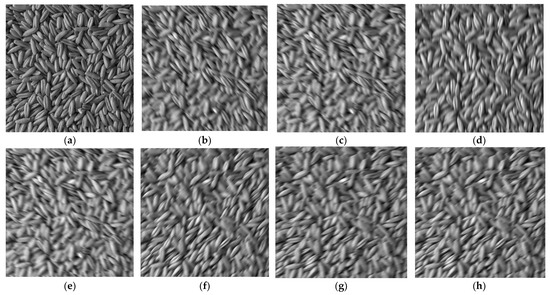
Figure 9.
(a) Test image “Oats”; (b–h) directionally filtered output images for the specified angles, respectively: (b) , (c) , (d) , (e) , (f) , (g) , and (h) .
Another relevant directional filtering is achieved on a grayscale image of 699 × 699 pixels, given in Figure 10a, which shows a view of a very narrow street between high buildings. The image is a cropped version of a photo taken from the free image database (“www.freepik.com” (accessed on 31 January 2024)), and its attribute is “hallway-building_26189437”. The image contains mainly straight lines representing architectural details; due to the narrow angle and the perspective effect, these lines appear oriented under various angles. The logarithmic FFT spectrum of the image has an interesting structure, very similar to the one in Figure 7b, consisting of fine, straight lines of various thicknesses and orientations corresponding to the various straight lines in the image.
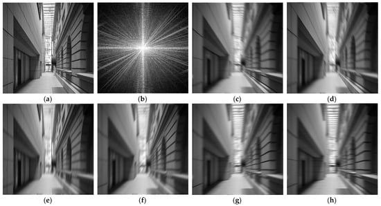
Figure 10.
(a) Grayscale test image “Street”; (b) its logarithmic FFT spectrum magnitude; and (c–h) directionally filtered output images for orientation angles: (c) , (d) , (e) , (f) , (g) , and (h) .
Applying a very selective straight Gaussian directional filter with various orientation angles, the filtered images in Figure 10c–h result. For a specified orientation of the filter, different straight lines (various edges of the street and buildings) are outlined, while others have various degrees of blurring, each one according to its orientation.
A directional filtering on a driving scene image (a road image as seen by the driver) is shown in Figure 11. The image (a) shows a straight road with trees on both sides. Using a very selective directional filter with specified orientation angles, we obtained the filtered images (b–d), in which the white markings and also the white lines representing the road margins are detected. Setting the appropriate orientation angle, the left (b), right (c), and center (d) markings are detected. Using the angle , all vertical lines are detected (tree trunks, lateral fence, etc.). Thus, such directional filters may find applications in image analysis for computer vision.
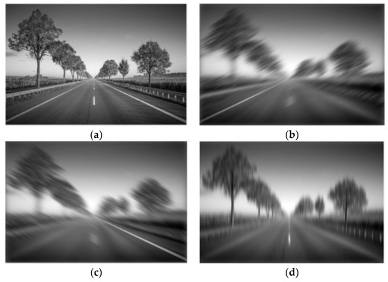
Figure 11.
(a) Driving scene image; directionally filtered images with orientation: (b) , (c) , and (d) .
4.2. Quantitative Evaluation of the Filtering Performance Using RMSE and PSNR
While the provided examples show the capabilities of directional filtering for the designed filters, it would be useful to evaluate their performance in a quantitative manner as well, using some objective metrics commonly applied in image processing. The most appropriate measures, in our case, would be the root mean squared error (RMSE) and, derived from it, the peak signal-to-noise ratio (PSNR), which is the ratio between the maximum value or power of a signal and the power of noise that affects the signal.
Since signals or images may have a very wide dynamic range, PSNR is most commonly expressed as a logarithmic quantity in decibels (dB).
Given a grayscale (monochrome) image unaffected by noise I and its noisy or otherwise distorted version J, RMSE is defined mathematically as:
Based on the root mean squared error, PSNR (in decibels) is given by the following expression:
In the above formula, is the maximum possible pixel value of the image. In the most common situation, when pixels are represented on 8 bits, this value is 255.
In our case, all the test images used in filtering are not affected by noise. An objective measure for the directional filter performance could be obtained by comparing the output images resulting from the ideal directional filter and the effectively designed filter, both with the same specified orientation angle. Referring to the directional filter with the straight frequency response, we should compare the designed filters (like those shown in Figure 4) with their corresponding ideal counterparts (like the one displayed in Figure 2a,b). The effectively designed directional filter can be considered a distorted version of its ideal counterpart since its characteristic has a limited longitudinal bandwidth and possibly some small linearity distortions and a low-level ripple in the stopband region. Therefore, the output filtered image resulting from it will be a distorted version of the output image resulting from the corresponding ideal filter with the same orientation angle. Thus, in calculating the RMSE and PSNR, the noisy image in (38) will be assimilated to the effectively filtered image but will be somewhat distorted as compared to the ideal image .
Next, we will quantitatively evaluate the filtering performance of the designed anisotropic filter with high selectivity (narrow frequency response), designed in Section 3.3 and based on the prototype given by frequency response (5), by comparing it with the filtering result using the ideal filter version of the form (7).
The directional filter’s orientation angle was varied in the range between 0 and with a small step, specifically , and for each orientation, the RMSE and PSNR were calculated with Equations (38) and (39). Their values are displayed in Table 1 and also represented graphically as bar plots in Figure 12. It can be noticed that the RMSE has a minimum value (0.434), and the corresponding PSNR has a maximum value (54.44 dB) for the orientation angle around . This indicates that for this angle, the overall level of distortion (due to the longitudinal band limitation, ripple, etc.) is minimal. As explained in a previous section, it is sufficient to design directional filters in this angle range; a filter with any other orientation can be obtained by simple symmetry operations.

Table 1.
Values of RMSE and PSNR (in dB) for orientation angles varying from 0 to in steps of .
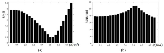
Figure 12.
(a) Bar plot of RMSE for specified orientation angle; (b) bar plot of PSNR for specified orientation angle.
5. Efficient Implementation of the 2D Anisotropic FIR Filters Using Polyphase and Block-Filtering Approach
Next, an efficient implementation with a low arithmetic complexity and a high degree of parallelism is developed at a system level for the designed 2D directional FIR filters, employing a polyphase structure that achieves a 2D filtering task with a relatively large convolution kernel (of size ). In order to implement the convolution operation with a kernel of this size, a block-filtering technique [48], combined with a polyphase decomposition, will be used.
As a preliminary step, employing sub-expression sharing methods, an algorithm that performs 2D filtering with a kernel of size 5 × 5 was developed, as presented below. To achieve this task, the kernel of the 2D filter obtained from the design and the input image to be filtered are decimated by factors 5 and 9, respectively; after this, a polyphase filtering technique is used. Through this approach, four partial output component images are calculated in parallel, namely , , , and , given by Equations (40)–(43) as follows:
in which the block matrices have the following form:
and , , and are the zero matrices of the sizes 5 × 15, 15 × 5, and 15 × 9, respectively. Summing up the partial results , , , and , resulting from (40)–(43), the following output vector containing 25 samples of the filtered image is obtained:
The vector appearing in Equations (40)–(43) is given below:
while the input vector is displayed as follows:
The main objective of the proposed 2D FIR polyphase filtering algorithm was to reduce the computational complexity and simultaneously speed up the calculation using a parallel filtering structure. It is widely acknowledged that applying a direct 2D convolution involves a high level of redundancy in computation due to overlapping blocks of input data; eliminating a large amount of such unnecessary, redundant calculations will result in a significant decrease in the arithmetic complexity of the system.
From this point on, the 2D filtering algorithm discussed above, for a simpler case, will be extended from an elementary kernel of size 5 × 5 to a larger kernel (31 × 31). In order to reach this aim and to obtain an efficient parallel computational structure, block processing combined with a polyphase technique will be further used.
Within the framework of this 2D polyphase structure, a decimation with a factor of 5 of the filter kernel will be performed. However, prior to decimation, the kernel has to be enlarged up to a size multiple of 5, in our case 35 × 35, by bordering it symmetrically with zeros at the margins. Meanwhile, a decimation by a factor of 9 was also applied to the input image, and in this way, an input image of the size 63 × 63 was obtained.
Employing the above-mentioned block processing and polyphase decomposition, as shown before, the following efficient algorithm has been derived for the implementation of the designed 2D FIR filter.
Thus, for the particular case where the kernel matrix is 15 × 15, and the input matrix is 27 × 27, the vectors , , , , , , …, , , …, , , …, , , …, will have the generic form given below (for , ):
For example, the vectors , , and generated by formula (48) will be:
For a simpler explanation of the proposed filtering algorithm, it was first demonstrated in a particular case of lower complexity, where the filter kernel is of the size 15 × 15, while the input image is of the size 27 × 27. Nevertheless, the results can be easily extended for the kernel of the directional FIR filter designed before, of the size 31 × 31, extended to the size 35 × 35 (by bordering with zeros), to be able to perform the decimation with a factor of 5.
Next, the simpler algorithm presented above for a 2D filter with a 5 × 5 kernel and 9 × 9 input matrix can be readily extended by achieving a decimation of the filter kernel by a factor of 5 and a decimation of the input matrix by a factor of 9. Thus, by decimating with a factor of 5, instead of the kernel with the size 15 × 15, 25 matrices of size 3 × 3 are obtained. As an example, for matrix , after decimating by 5, a block matrix of size 3 × 3 will result as follows:
Next, by concatenating the rows of matrix , the matrix is derived from Equation (46). The vector is also substituted with the vector given by (47).
The vectors ,,,, …, , which compose matrix and are given by the input image, are defined by the general indexed expression as follows:
For instance, the vectors ,, resulting from formula (51) will be:
The vectors , , , , …, have been determined as described next. For the purpose of easier understanding, our demonstration considers the simpler case in which the input image is of size 27 × 27 and is decimated by a factor of 9. As a result, instead of the input matrix of size 27 × 27, a number of 81 matrices of size 3 × 3 are derived. Taking the case of as an example, through decimation by a factor of 9, the following 3 × 3 block matrix results are as follows:
Next, the rows of will be concatenated, then the obtained vector is reversed, and finally, the vector is derived from the general Equation (51):
Although the algorithm presentation was restricted to a particular situation where the input matrix is of the size 27 × 27, for an easier understanding, it is also straightforward to apply it in a more general case. For instance, a 2D FIR filtering with a 5 × 5 kernel applied to a 9 × 9 input image matrix was decomposed into 225 1D inner products using the following block matrix equations:
Finally, the following output vector will be derived:
In Equations (55)–(58), the block matrices are, respectively, , where the vector , and , where is the identity matrix (with ones on the main diagonal and zeros elsewhere); we also have . The matrices , , and are null matrices of the sizes 5 × 135, 135 × 45, and 135 × 81, respectively.
6. Discussion
The analytical design technique proposed here for anisotropic Gaussian 2D FIR filters is relatively simple and efficient. Two types of such filters have been approached, with straight and elliptical shapes of the frequency response. As shown in the provided examples, the filters designed through this method have a precise shape with negligible distortions, good linearity along the axes, and wide longitudinal bandwidths. Since they are of the FIR type, these filters are unconditionally stable. Because they are derived from a Gaussian prototype with a real-values transfer function, these filters have a zero phase, which is a desirable feature due to the absence of phase distortions in the filtered image.
A very rigorous comparison regarding performance with directional filters already existing in the literature is quite difficult to make because such filters differ very much in terms of their shape, specifications, and applications. Only some qualitative, general comparative remarks can be made. The analytically designed Gaussian straight directional filter is very selective at a relatively low order (due to the efficient approximation used) compared to other similar filters from the literature. Furthermore, the characteristics and associated contours given in Figure 4 for several orientations show a straight, linear response in the frequency plane, with a visibly wider longitudinal bandwidth, compared with the Gaussian filter using triple-axis decomposition [8] and also the Gaussian smoothing filters in [9,10] with an elliptical shape in the frequency plane.
The advantages of the proposed design technique for these 2D directional filters, which also apply to other types of 2D filters, as presented in [49,50,51,52,53,54], were highlighted in detail in Section 2.1. The most important one would be the flexibility in design due to the fact that the resulting 2D filters have a parametric, factored frequency response, which allows them to be easily tuned and adjusted according to given specifications. The 2D filters derived through frequency mapping inherit the properties of the 1D prototype, and therefore, their shape is exactly controlled and has low distortions and wide longitudinal bandwidths. This ensures a high directional selectivity and makes them suitable for the tasks detailed in Section 4, namely the detection and extraction of oriented lines and other objects from various images—a useful application that has not been approached by other researchers in the image processing field. In regards to the implementation, our novel solution based on polyphase and block filtering ensures a low computational complexity. We have not found any implementation of a 2D filter with the same degree of parallelism in the literature (computing 25 image samples simultaneously).
A comparison can also be made with the first author’s previous works approaching related design methods [49,50,51,52,53,54]. In [49], a class of adjustable Gaussian filters is proposed, but they are of IIR type. While IIR filters are generally of lower order than FIR for similar specifications and, thus, are more computationally efficient, their stability must be ensured for correct operation, which sometimes may be quite difficult. In [50,51], other directional IIR filters, based on different prototypes, are designed analytically. In [52], the proposed directional Gaussian FIR filters using separability and decomposition along three frequency axes have low orders, but their longitudinal bandwidth is narrower. Also, the method used in [52] is more elaborate and difficult to apply. By comparison, the filters developed in the current work do not use 2D Gaussian separability, but they have much wider longitudinal bandwidths, and consequently, their directional selectivity is better; the applied method is also significantly simpler.
The proposed 2D anisotropic directional filters have the advantage of being parametric and, therefore, adjustable. For straight-shaped filters, matrix in (19) depends on the orientation angle , as in (20), and so does the overall filter kernel . For elliptically shaped filters, matrix in (35) depends both on the angle and ellipse semi-axes (E, F), according to (36). Thus, for any specified parameter values, the filter matrices are derived directly. This is one advantage of the analytical approach: The design procedure need not be resumed every time from the beginning when changing the parameters—they are simply substituted in the filter matrices.
Regarding the implementation part, the proposed polyphase block-filtering algorithm continues the algorithm from [54] but is superior in efficiency. It has a higher degree of parallelism and different decimation factors and, therefore, performs better regarding computational complexity, as discussed below. We make a brief comparison between the direct convolution and the polyphase filtering technique proposed above in terms of arithmetic complexity. As is widely known, a 2D filtering of an image with pixels, with a FIR filter having a kernel of the size implies a 2D convolution operation between a matrix and a matrix. As the filter kernel overlaps with the image sliding along the two axes, each pixel requires multiplications; therefore, the overall 2D filtering requires, in total, multiplications. Also, it is easy to evaluate the total number of additions .
In this simplified, demonstrative approach, we used 25 inner products, each implying multiplications and additions, giving in total multiplications and 225 additions, plus 660 additions in the pre-processing stage and additions in the post-processing stage.
The 2D directional filter effectively designed in Section 3.3 has a kernel of size ; in order to obtain a polyphase decomposition with a decimation factor of 5, we need to extend the kernel to size by adding four columns and rows of zeros. In this case, we need multiplications and 4225 additions, plus 660 additions in the pre-processing stage and 135 additions in the post-processing stage.
Aside from a reduction in the arithmetic complexity, a significant speed improvement can be achieved by using a parallel implementation. Thus, we can compute 25 samples simultaneously and 100 computations can be done in parallel, and the partial results are added to obtain those 25 samples in parallel.
7. Conclusions
The proposed design procedure for the two types of 2D Gaussian anisotropic filters is totally analytic, based on 1D prototypes, approximations, and frequency mappings, thus avoiding the use of global numerical optimization. The design is simple and efficient, leading to 2D FIR filters with an accurate shape and factored frequency response. The obtained 2D filters are parametric, and their specifications (selectivity and orientation angle) appear explicitly in the filter matrix; therefore, they are easily adjustable. Simulations show the capability of very selective directional filters to detect and extract straight lines and other various oriented details from images, with potential applications in fields like computer vision, object recognition, etc. The developed parallel implementation, using a polyphase and block processing structure, yields efficient 2D filters, minimizing the arithmetic complexity. In further work on this topic, the authors will investigate how to improve and extend the design method to obtain various anisotropic filters, find new applications, and also to obtain more efficient filter implementations.
Author Contributions
Conceptualization, R.M. and D.F.C.; methodology, R.M. and D.F.C.; software, D.F.C. and R.M; validation, D.F.C. and R.M.; formal analysis, D.F.C. and R.M.; investigation, R.M. and D.F.C.; resources, D.F.C. and R.M.; writing—original draft preparation and writing—review and editing, R.M. and D.F.C.; project administration, D.F.C.; funding acquisition, D.F.C. All authors have read and agreed to the published version of the manuscript.
Funding
This research received no external funding.
Institutional Review Board Statement
Not applicable.
Informed Consent Statement
Not applicable.
Data Availability Statement
All data underlying the results are available as part of the article, and no additional source data are required.
Conflicts of Interest
The authors declare no conflicts of interest.
References
- Lu, W.; Antoniou, A. Two-Dimensional Digital Filters; CRC Press: Boca Raton, FL, USA, 1992. [Google Scholar]
- Najim, M. (Ed.) Digital Filters Design for Signal and Image Processing; Wiley: Hoboken, NJ, USA, 2006. [Google Scholar]
- Woods, J.W. Multidimensional Signal, Image, and Video Processing and Coding, 2nd ed.; Academic Press: Cambridge, MA, USA, 2011. [Google Scholar]
- Chen, C.-K.; Ju-Hong, L. McClellan transform based design techniques for two-dimensional linear-phase FIR filters. IEEE Trans. Circuits Syst. I Fundam. Theory Appl. 1994, 41, 505–517. [Google Scholar] [CrossRef]
- Young, I.T.; van Vliet, L.J. Recursive implementation of the Gaussian filter. Signal Process. 1995, 44, 139–151. [Google Scholar] [CrossRef]
- Geusebroek, J.-M.; Smeulders, A.W.M.; van de Weijer, J. Fast anisotropic Gauss filtering. IEEE Trans. Image Process. 2003, 12, 938–943. [Google Scholar] [CrossRef]
- Lampert, C.H.; Wirjadi, O. An optimal nonorthogonal separation of the anisotropic Gaussian convolution filter. IEEE Trans. Image Process. 2006, 15, 3501–3513. [Google Scholar] [CrossRef] [PubMed][Green Version]
- Lam, S.Y.M.; Shi, B.E. Recursive anisotropic 2-D Gaussian filtering based on a triple-axis decomposition. IEEE Trans. Image Process. 2007, 16, 1925–1930. [Google Scholar] [PubMed]
- Lakshmanan, V. A separable filter for directional smoothing. IEEE Geosci. Remote Sens. Lett. 2004, 1, 192–195. [Google Scholar] [CrossRef]
- Charalampidis, D. Efficient directional Gaussian smoothers. IEEE Geosci. Remote Sens. Lett. 2009, 6, 383–387. [Google Scholar] [CrossRef]
- Paplinski, A.P. Directional filtering in edge detection. IEEE Trans. Image Process. 1998, 7, 611–615. [Google Scholar] [CrossRef]
- Hsiao, P.-Y.; Chen, C.-H.; Chou, S.-S.; Li, L.-T.; Chen, S.-J. A parameterizable digital-approximated 2D Gaussian smoothing filter for edge detection in noisy image. In Proceedings of the IEEE International Symposium on Circuits and Systems (ISCAS), Kos, Greece, 21–24 May 2006. [Google Scholar]
- Austvoll, I. Directional filters and a new structure for estimation of optical flow. In Proceedings of the 2000 International Conference on Image Processing, Vancouver, BC, Canada, 10–13 September 2000; Volume 2, pp. 574–577. [Google Scholar] [CrossRef]
- Nguyen, T.T.; Oraintara, S. Multiresolution direction filterbanks: Theory, design, and applications. IEEE Trans. Signal Process. 2005, 53, 3895–3905. [Google Scholar] [CrossRef]
- Stavrou, V.N.; Tsoulos, I.G.; Mastorakis, N.E. Transformations for FIR and IIR filters’ design. Symmetry 2021, 13, 533. [Google Scholar] [CrossRef]
- Apostolov, P.S.; Yurukov, B.P.; Stefanov, A.K. An easy and efficient method for synthesizing two-dimensional finite impulse response filters with improved selectivity. IEEE Signal Process. Mag. 2017, 34, 180–183. [Google Scholar] [CrossRef]
- Aggarwal, A.; Kumar, M.; Rawat, T.K. Design of two-dimensional FIR filters with quadrantally symmetric properties using the 2D L1-method. IET Signal Process. 2019, 13, 262–272. [Google Scholar] [CrossRef]
- Capizzi, G.; Sciuto, G.L. A novel 2-D FIR filter design methodology based on a Gaussian-based approximation. IEEE Signal Process. Lett. 2019, 26, 362–366. [Google Scholar] [CrossRef]
- Pei, S.C.; Huang, S.G. 2-D Laguerre distributed approximating functional: A circular low-pass/band-pass filter. IEEE Trans. Circuits Syst. II Express Briefs 2019, 66, 818–822. [Google Scholar] [CrossRef]
- Kwan, H.K.; Zhang, M. 2-D linear phase FIR digital filter design using TLBO. In Proceedings of the IEEE 23rd International Conference on Digital Signal Processing (DSP), Shanghai, China, 19–21 November 2018; pp. 1–4. [Google Scholar] [CrossRef]
- Bindima, T.; Elias, E. Low-complexity 2-D digital FIR filters using polyphase decomposition and Farrow structure. IEEE Trans. Circuits Syst. I Regul. Pap. 2019, 66, 2298–2308. [Google Scholar] [CrossRef]
- Hussain, M.; Jenkins, W.K.; Radhakrishnan, C. Use of the Lévy flight firefly algorithm in 2D McClellan unconstrained transform adaptive filters. In Proceedings of the IEEE 63rd International Midwest Symposium on Circuits and Systems (MWSCAS), Springfield, MA, USA, 9–12 August 2020; pp. 856–859. [Google Scholar] [CrossRef]
- Yadav, S.; Yadav, R.; Kumar, A.; Kumar, M. Design of optimal two-dimensional FIR filters with quadrantally symmetric properties using Vortex Search Algorithm. J. Circuits Syst. Comput. 2020, 29, 2050155. [Google Scholar] [CrossRef]
- Zhang, X.; Xiong, Q.; Xu, X. A multimodal biometric recognition algorithm based on second generation curvelet and 2D Gabor filter. In Proceedings of the 2019 4th International Conference on Control, Robotics and Cybernetics (CRC), Tokyo, Japan, 27–30 September 2019; pp. 114–117. [Google Scholar] [CrossRef]
- Kim, J.; Um, S.; Min, D. Fast 2D complex Gabor filter with kernel decomposition. IEEE Trans. Image Process. 2018, 27, 1713–1722. [Google Scholar] [CrossRef] [PubMed]
- Chen, W.T.; Chen, P.Y.; Hsiao, Y.C.; Lin, S.H. A low-cost design of 2D median filter. IEEE Access 2019, 7, 150623–150629. [Google Scholar] [CrossRef]
- Froehly, A.; Herschel, R. Detection of fiber orientation with SAR imaging via amplitude and phase filtering. In Proceedings of the 18th European Radar Conference (EuRAD), London, UK; 2022; pp. 261–264. [Google Scholar] [CrossRef]
- Suresh, S.; Lal, S. Two-dimensional CS adaptive FIR Wiener filtering algorithm for the denoising of satellite images. IEEE J. Sel. Top. Appl. Earth Obs. Remote Sens. 2017, 10, 5245–5257. [Google Scholar] [CrossRef]
- Porzycka-Strzelczyk, S.; Rotter, P.; Strzelczyk, J. Automatic detection of subsidence troughs in SAR interferograms based on circular Gabor filters. IEEE Geosci. Remote Sens. Lett. 2018, 15, 873–876. [Google Scholar] [CrossRef]
- Zhang, Z.; Bian, H.; Song, Z. A multi-view sonar image fusion method based on the morphological wavelet and directional filters. In Proceedings of the IEEE/OES China Ocean Acoustics (COA), Harbin, China, 9–11 January 2016; pp. 1–6. [Google Scholar] [CrossRef]
- Wu, Z.; Jin, Y.; Yi, K.M. Neural Fourier filter bank. In Proceedings of the IEEE/CVF Conference on Computer Vision and Pattern Recognition (CVPR), Vancouver, BC, Canada, 18–22 June 2023; pp. 14153–14163. [Google Scholar] [CrossRef]
- Vasconcelos, C.N.; Oztireli, C.; Matthews, M.; Hashemi, M.; Swersky, K.; Tagliasacchi, A. CUF: Continuous upsampling filters. In Proceedings of the IEEE/CVF Conference on Computer Vision and Pattern Recognition (CVPR), Vancouver, BC, Canada, 18–22 June 2023. [Google Scholar] [CrossRef]
- Struiksma, R.E.; Uysal, F.; van Rossum, W.L. 2D matched filtering with time-stretching; application to orthogonal matching pursuit (OMP). In Proceedings of the 2021 18th European Radar Conference (EuRAD), London, UK, 5–7 April 2022; pp. 249–252. [Google Scholar] [CrossRef]
- Li, Q.; Wang, Q.; Li, X. Exploring the relationship between 2D/3D convolution for hyperspectral image super-resolution. IEEE Trans. Geosci. Remote Sens. 2021, 59, 8693–8703. [Google Scholar] [CrossRef]
- Astola, J.; Neuvo, Y.; Rusu, C. On two-dimensional polynomial predictors. In Proceedings of the 28th European Signal Processing Conference (EUSIPCO), Amsterdam, The Netherlands, 18–21 January 2021; pp. 2254–2258. [Google Scholar] [CrossRef]
- Sreelekha, K.R.; Bindiya, T.S. A new multiplier-free transformation for the design of hardware efficient circularly symmetric wideband 2D filters. In Proceedings of the TENCON 2019-2019 IEEE Region 10 Conference (TENCON), Kochi, India, 17–20 October 2019; pp. 2376–2381. [Google Scholar] [CrossRef]
- Pei, S.-C.; Chang, K.-W. Two dimensional efficient multiplier-less structures of Möbius function for Ramanujan filter banks. IEEE Trans. Signal Process. 2020, 68, 5079–5091. [Google Scholar] [CrossRef]
- Antoniou, G.E.; Coutras, C.A. 2D lattice FIR digital filter with alternate delays: Minimal circuit and state-space realization. In Proceedings of the 2021 International Symposium on Signals, Circuits and Systems (ISSCS), Iasi, Romania, 15–16 July 2021; pp. 1–4. [Google Scholar] [CrossRef]
- Antoniou, G.E.; Bardis, N.; Gonos, I.; Coutras, C. New 2D FIR direct-form minimal circuit and state-space filter structures. In Proceedings of the 2022 12th International Conference on Dependable Systems, Services and Technologies (DESSERT), Athens, Greece, 9–11 December 2022. [Google Scholar] [CrossRef]
- Licciardo, G.D.; Cappetta, C.; Di Benedetto, L. FPGA optimization of convolution-based 2D filtering processor for image processing. In Proceedings of the 8th Computer Science and Electronic Engineering, Colchester, UK, 28–30 September 2016; pp. 180–185. [Google Scholar] [CrossRef]
- Rybenkov, E.V.; Petrovsky, N.A. High performance multiplier-less pipelined FPGA architecture for 2-D non-separable quaternionic filter banks. In Proceedings of the 2020 Signal Processing: Algorithms, Architectures, Arrangements, and Applications (SPA), Poznan, Poland, 23–25 September 2020; pp. 42–47. [Google Scholar] [CrossRef]
- Cheemalakonda, S.; Chagarlamudi, S.; Dasari, B.; Sulthana, S.S.; Gundugonti, K.K. Area efficient 2D FIR filter architecture for image processing applications. In Proceedings of the 6th International Conference on Devices, Circuits and Systems (ICDCS), Coimbatore, India, 21–22 April 2022; pp. 337–341. [Google Scholar] [CrossRef]
- Samanth, R.; Kedlaya, V.; Nayak, S.G. A novel approach to develop low power MACs for 2D image filtering. IEEE Access 2021, 9, 28421–28428. [Google Scholar] [CrossRef]
- Lyakhov, P.A.; Abdulsalyamova, A.S.; Semyonova, N.F.; Nagornov, N.N.; Voznesensky, A.S.; Kaplun, D.I. On the computational complexity of 2D filtering by Winograd method. In Proceedings of the 11th Mediterranean Conference on Embedded Computing (MECO), Budva, Montenegro, 7–10 June 2022; pp. 1–4. [Google Scholar] [CrossRef]
- Bistritz, Y. Bounded-input bounded-output stability tests for two-dimensional continuous-time systems. IEEE Trans. Circuits Syst. I Regul. Pap. 2021, 68, 2134–2147. [Google Scholar] [CrossRef]
- Aggarwal, N.; Karl, W. Line detection in images through regularized Hough transform. IEEE Trans. Image Process. 2006, 15, 582–591. [Google Scholar] [CrossRef] [PubMed]
- Li, C.; Wang, Z.; Li, L. An improved HT algorithm on straight line detection based on Freeman chain code. In Proceedings of the 2009 2nd International Congress on Image and Signal Processing, Tianjin, China, 17–19 October 2009; pp. 1–4. [Google Scholar] [CrossRef]
- Aziz, M.; Boussakta, S.; McLernon, D.C. High performance 2D parallel block-filtering system for real-time imaging applications using the Sharc ADSP21060. Real-Time Imaging 2003, 9, 151–161. [Google Scholar] [CrossRef]
- Matei, R. Design of 2D parametric filters for directional Gaussian smoothing. In Proceedings of the 21st European Conference on Circuit Theory and Design, ECCTD’13, Dresden, Germany, 8–12 September 2013. [Google Scholar] [CrossRef]
- Matei, R. Analytic design of directional and square-shaped 2D IIR filters based on digital prototypes. Multidimens. Syst. Signal Process. 2019, 30, 2021–2043. [Google Scholar] [CrossRef]
- Matei, R. A class of directional zero-phase 2D filters designed using analytical approach. IEEE Trans. Circuits Syst. I Regul. Pap. 2022, 69, 1629–1640. [Google Scholar] [CrossRef]
- Matei, R. Analytical design methods for directional Gaussian 2D FIR filters. Multidimens. Syst. Signal Process. 2018, 29, 185–211. [Google Scholar] [CrossRef]
- Matei, R. Design and Applications of Adjustable 2D Digital Filters with Elliptical and Circular Symmetry. Analog. Integr. Circuits Signal Process. 2023, 114, 345–358. [Google Scholar] [CrossRef]
- Matei, R.; Chiper, D.F. Analytic design technique for 2D FIR circular filter banks and their efficient implementation using polyphase approach. Sensors 2023, 23, 9851. [Google Scholar] [CrossRef] [PubMed]


Disclaimer/Publisher’s Note: The statements, opinions and data contained in all publications are solely those of the individual author(s) and contributor(s) and not of MDPI and/or the editor(s). MDPI and/or the editor(s) disclaim responsibility for any injury to people or property resulting from any ideas, methods, instructions or products referred to in the content. |
© 2024 by the authors. Licensee MDPI, Basel, Switzerland. This article is an open access article distributed under the terms and conditions of the Creative Commons Attribution (CC BY) license (https://creativecommons.org/licenses/by/4.0/).