Development of an Integrated Longitudinal Control Algorithm for Autonomous Mobility with EEG-Based Driver Status Classification and Safety Index

Abstract

During unexpected driving situations in autonomous vehicles, such as a system failure, the driver should take over control from the vehicles in SAE Level 3 to cope with unexpected situations. Therefore, it is necessary to develop reasonable takeover technologies to ensure safe driving. In this study, an electroencephalogram (EEG)-based driver status classification model and a safety index-based integrated longitudinal control algorithm considering the takeover time and driving characteristics are proposed. The driver status is classified into two states: road monitoring and non-driving-related tasks. EEG data are acquired while the driver performs certain tasks. The driver status classification model is presented using the EEG data based on a machine learning method. It is designed such that the desired takeover time is determined based on the classified driver state. To design the integrated longitudinal control algorithm, a safety index is designed and calculated based on the vehicle state and driver’s driving characteristics. The desired clearances based on the desired takeover time and driver characteristics are calculated and selected based on the safety index. A sliding-mode control algorithm is adopted to allow the vehicle to track the desired clearance reasonably. The performance of the proposed control algorithm is evaluated using the MATLAB/Simulink R2019a (Mathworks, Natick, Massachusetts, U.S.A) and CarMaker software 8.1.1 (IPG Automotive, Karlsruhe, Germany).

1. Introduction

At SAE Level 2, advanced drive assistance system (ADAS)-based driving assist technologies such as lane-keeping, cruise control, and collision avoidance have been commercialized. Recently, a conditional automation system has been prepared for commercialization as SAE Level 3. In SAE Level 3, the driver is not required to monitor the road and is guaranteed to engage in various activities in the cabin. The driver should take over control and cope with unexpected situations when the vehicle system requires, such as in the case of system failure. If the driver takes over control while being distracted or not concentrating, they can take over unstably by applying unnecessary steering or acceleration/brake pedal inputs, which can lead to accidents caused by driver negligence. Previous research has confirmed that takeover times differ depending on driver age and tasks (for example, watching a video, listening to music, or playing mobile games) [1,2,3,4,5]. Although the driver status affects the ability to take control, the current ADAS-based autonomous driving assistance system performs assist driving or semi-autonomous driving without considering the driver status. Therefore, it is essential to execute takeover considering the driver status, and ISO and UNECE require driver monitoring systems (DMSs) in autonomous vehicles for safe and stable takeovers. Although various methods have been suggested for monitoring driver status, most studies have been conducted to detect or determine drowsiness, distraction, and mental workload.

Kouchak et al. proposed a distraction detection method that uses long short-term memory in various driving scenarios [6]. Meng et al. proposed a driver drowsiness detection algorithm and classified drowsiness levels for driver monitoring [7]. Driver monitoring has been generally conducted to detect driver distractions or drowsiness using vehicle states such as speed, acceleration, pedal inputs, and steering wheel inputs. Furthermore, it has been used to classify driver behaviors as normal or aggressive. Shagverdy et al. proposed a driver behavior classification model that recognizes normal, aggressive, distracted, drowsy, and drunken [8]. Lattanzi et al. proposed a safe and unsafe driving behavior classification model using machine learning (ML) techniques [9]. Because the aforementioned methodologies are based on vehicle states, it is difficult to use them for DMSs in autonomous vehicles that must make decisions and respond quickly before taking over.

Various driver monitoring methodologies have been utilized driver vital information. A driver situational awareness decision algorithm based on an intelligent fuzzy-based DMSs was proposed using the respiratory rate in [10]. Electrocardiogram and electrodermal activity measurements were used to monitor driver conducting non-driving-related tasks (NDRTs), 2-back, by generating a mental workload in [11]. Persson et al. proposed a driver sleepiness classification algorithm using the heart rate and analyzed its sensitivity by comparing the performances of ML methods [12]. Cardon et al. proposed a classification algorithm for driver mental workload levels using infrared thermal images and heart rate variabilities [13]. In addition, DMSs that use EEG data have been developed to detect fatigue, drowsiness, and distraction in autonomous vehicles [14]. Li et al. proposed a driver distraction detection algorithm using a convolutional neural network (CNN) by analyzing the EEG while the driver conducts secondary tasks (for example, cellphones and 2-back) [15]. Gao et al. proposed a spatiotemporal CNN-based classification model for detecting driver fatigue [16]. Zeng et al. developed a driver mental state classification model by dividing the mental state into eight stages [17]. In [18,19,20], a driver drowsiness detection model was proposed using a learning method, TSK fuzzy system, interpretable CNN, and deep neural network. Jiao et al. suggested a driver sleepiness detection model using EEG and electrooculography signals using a network methodology [21]. Yang et al. developed a driver fatigue detection model by classifying driver status into fatigue and alertness [22]. Research on the detailed classification of driver behavior has primarily been conducted using cameras. Martin et al. suggested a driver behavior recognition algorithm for autonomous vehicles using body and head poses, depth, and interior information from six views of depth cameras [23]. Xing et al. proposed a CNN-based driver activity recognition algorithm for autonomous vehicles using a low-cost camera [24]. The aforementioned studies have classified driver activities into reading, texting, mobile phone use, and side mirror checking. Kose et al. proposed a camera RGB-information-based driver state-monitoring algorithm by classifying driver distraction levels and movement decisions in autonomous vehicles [25]. In addition, driver behavior was analyzed by tracking eye glances using a camera in an autonomous vehicle in [26,27]. In [28], driver behavior indices were suggested to categorize travel patterns, abnormal driving, reaction time, and braking patterns using vision and telematic sensors. Li et al. investigated the effects of NDRTs by analyzing the eye-movement patterns of drivers during autonomous driving [29]. However, when monitoring driver behavior using a camera, the driver must always be within the camera’s field of view and avoid behaviors that can cover the driver’s face or body from the camera.

In autonomous driving technology, obstacle avoidance systems are also important in securing safety, but other technologies should be developed based on systems to prevent collisions first. Therefore, this study aims to develop an algorithm that prioritizes safety to prevent collisions based on the driving characteristics and driver status, determining the vehicle time headway and the desired take-over time, respectively. Because EEGs have information about human behavior intentions [30], an EEG-based driver status monitoring algorithm is proposed in this study for the safe takeover of autonomous mobility by detecting driver status. Additionally, a longitudinal control algorithm is designed to ensure the desired takeover time (TOT) based on the classified driver status. ML methods such as artificial neural networks (ANNs), recurrent neural networks (RNNs), and support vector machines (SVMs) are employed to classify the driver status for road monitoring and NDRT using EEG data. Subsequently, the desired TOT is determined based on the classified driver status, and the desired clearance is calculated to ensure the desired TOT under a car-following situation. The integrated desired clearance is designed to consider the desired TOT and driving characteristics and is determined based on a safety index calculated with vehicle states. Although the sliding mode control (SMC) has a chattering phenomenon, it is usually utilized for nonlinear system control because it can be designed relatively easily and ensures real-time control. In addition, it can guarantee not only stability but also robustness in situations in which various disturbances exist. Therefore, the SMC is used to track the integrated desired clearance by computing the desired longitudinal acceleration for robust longitudinal safety in takeover situations of autonomous vehicles. The main contributions of this paper are summarized as follows:

• The EEG-based driver status classification algorithm is proposed, and the desired TOT is determined by considering the classified driver status.
• The longitudinal control algorithm considering the safety index calculated based on vehicle states is proposed to ensure the desired TOT and driving characteristics.

The performance of the proposed algorithm was verified using the MATLAB/Simulink R2019a and CarMaker software 8.1.1 in car-following scenarios.

The remainder of this paper is organized as follows. Section 2 presents a safety-index-based integrated longitudinal control with a driver status classification model. Performance evaluation was conducted using the MATLAB/Simulink R2019a and CarMaker software 8.1.1 under the car-following scenario described in Section 3. Finally, future work and conclusions are presented in Section 4.

2. Integrated Longitudinal Control Algorithm

In this section, a driver status classification and safety index-based integrated longitudinal control algorithm are established to ensure safe takeover for autonomous vehicles. The proposed algorithm comprises the desired TOT determination based on driver status, desired clearance calculation, desired clearance integration with the safety index, and a longitudinal controller using the SMC. Figure 1 depicts block diagrams of the proposed takeover and longitudinal control algorithm.

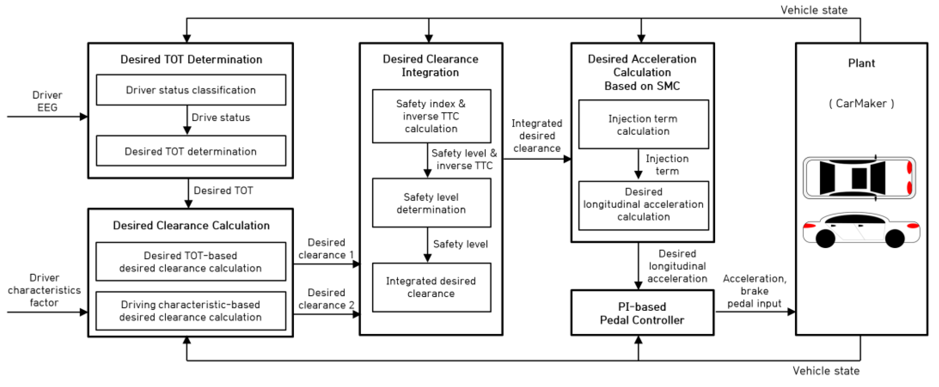
The driver status is determined using the driver’s EEG based on the ML method, and the desired TOT is determined based on the determined driver status. The desired clearance is calculated to ensure the desired TOT. The safety index is calculated considering the driving situation using the vehicle states, and the integrated desired clearance is calculated considering the desired TOT and driving characteristics. The SMC is designed to calculate the desired longitudinal acceleration and track the desired integrated clearance. A proportional–integral (PI) controller is utilized to control the acceleration and brake pedal to track the desired longitudinal acceleration calculated from the SMC and applied to the vehicle control input as the pedal input.

2.1. EEG-Based Driver Status Classification

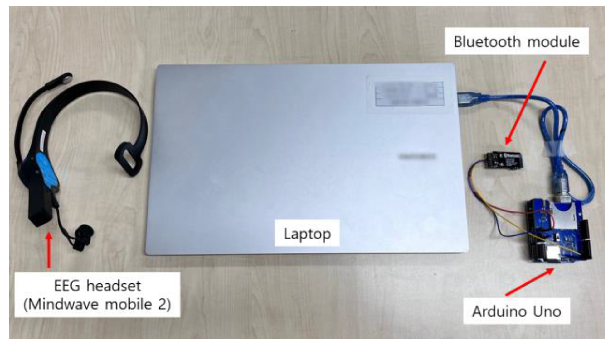
In this section, an EEGs in which drivers performed specific tasks are acquired and analyzed, and a driver status classification model using ML methods (that is, ANN, RNN, and SVM) is proposed. EEG data acquisition equipment and experiments are established in the design of the driver status classification process. The EEG data acquisition equipment is comprised of an EEG headset (NeuroSky MindWave Mobile 2), Bluetooth module, Arduino Uno, and laptop, as shown in Figure 2.

The EEG headset sends the EEG data to the Arduino Uno through Bluetooth at 1 Hz and saves them using a laptop. The acquired EEG data include the delta, theta, high alpha, low alpha, high beta, low beta, high gamma, and middle gamma waves, and their range of frequencies is in

Table 1. The range of EEG frequency.

Division	Value
Delta	<4 Hz
Theta	4–7 Hz
Low alpha	8–9 Hz
High alpha	10–12 Hz
Low beta	13–18 Hz
High beta	18–30 Hz
Low gamma	31–40 Hz
Middle gamma	<41 Hz

[31].

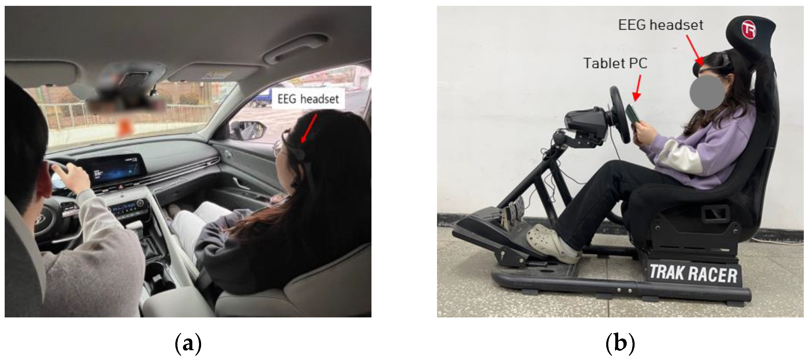
In the EEG data acquisition experiment, ten drivers participated (seven males and three females) with an average age of 25.1 years; they have driving licenses and different driving experiences. The experiment was conducted to acquire the driver EEG data for 5 min while the drivers were engaged in road monitoring or NDRT. Drivers were told to concentrate on the task that they were performing. The experimental environment was constructed using a real vehicle and driving simulator (Logitech G29), as shown in Figure 3.

As shown in Figure 3, the drivers wore the EEG headsets during road monitoring and NDRT. The driver performed road monitoring by getting into the passenger seat, assuming that they were in an autonomous vehicle. 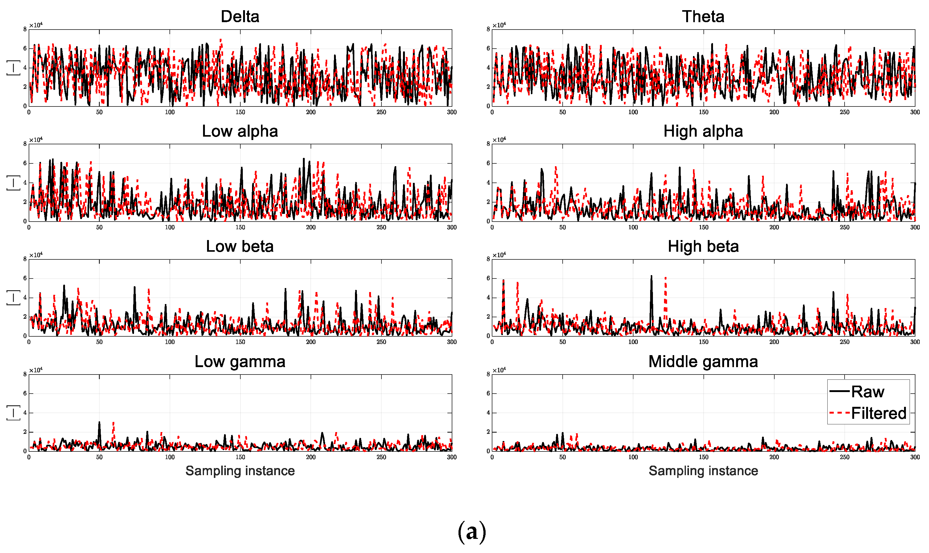Because watching movies is a common activity in autonomous vehicles and can cause driver distraction, affecting takeover ability, watching movies was applied as the NDRT in this study [29,32,33,34]. Owing to the driver being able to carry on various activities in autonomous vehicles, it is planned to acquire the EEG data in various situation and drivers such as conversations with passengers and reading books to establish the robustness and generalizability of the proposed driver status classification model in the future. The driver used a tablet PC to watch movies and videos during the experiment in the driving simulator. The EEG data during NDRT were acquired when the driver concentrated on the NDRT, and the experiment was conducted indoors to eliminate factors that could affect driver brain signals, such as car sickness or driving environment (traffic condition, ride comfort, etc.), during the acquisition process. In total, 100 EEG data points—delta, theta, high alpha, low alpha, high beta, low beta, high gamma, and middle gamma waves—were acquired, with 10 data points acquired from each person, and the Savitzky–Golay filter was utilized to smooth the acquired EEG data in real time. 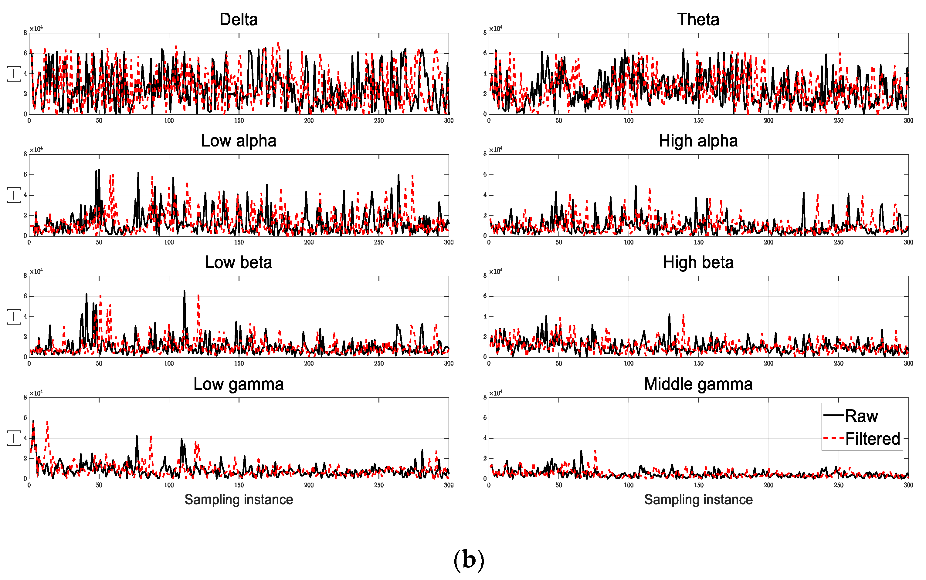Figure 4 shows the acquired raw data and smoothing of the EEG data, which is fitted of 11 data into a 5th-order polynomial function and selected the first of the fitted EEG data when the driver conducts road monitoring and NDRT.

As can be seen from Figure 4, since the raw or filtered data of the EEG is difficult to categorize between the two tasks, road monitoring and NDRT, there is a possibility that classification performance degradation can be occurred when the raw or filtered data of the EEG is used as an input for ML method. Therefore, a sliding window method is employed for feature extraction by calculating the standard deviation and difference between the maximum and minimum EEG data in the window. The standard deviations and differences in the window are expressed by Equation (1) and Equation (2), respectively:

$${\sigma }_{EEG}=\sqrt{\frac{\sum _{i=1}^N{\left(x_i-\mu \right)}^2}{N}}$$

(1)

$${\Delta x}_{EEG}=x_{max}-x_{min}$$

(2)

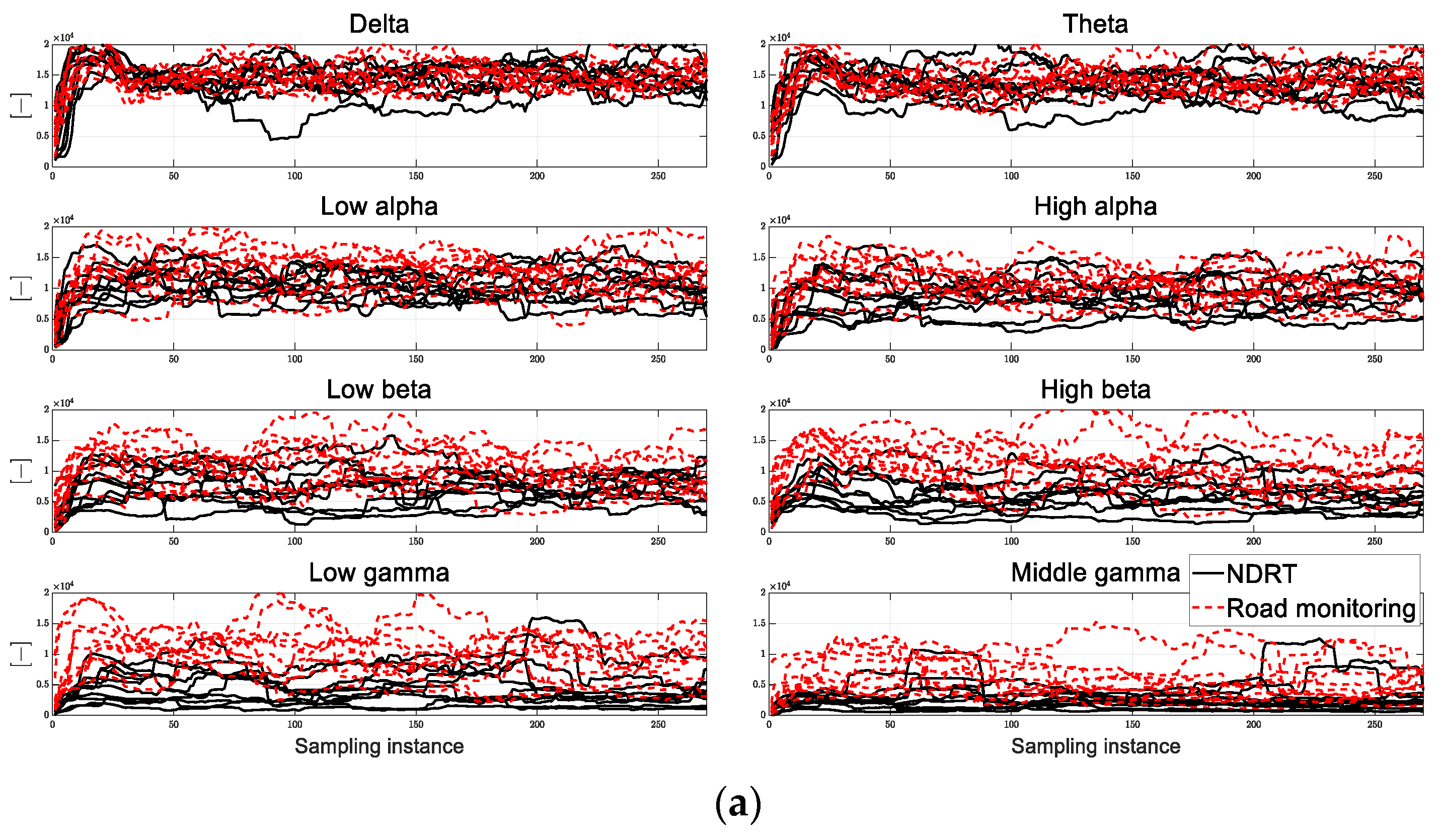
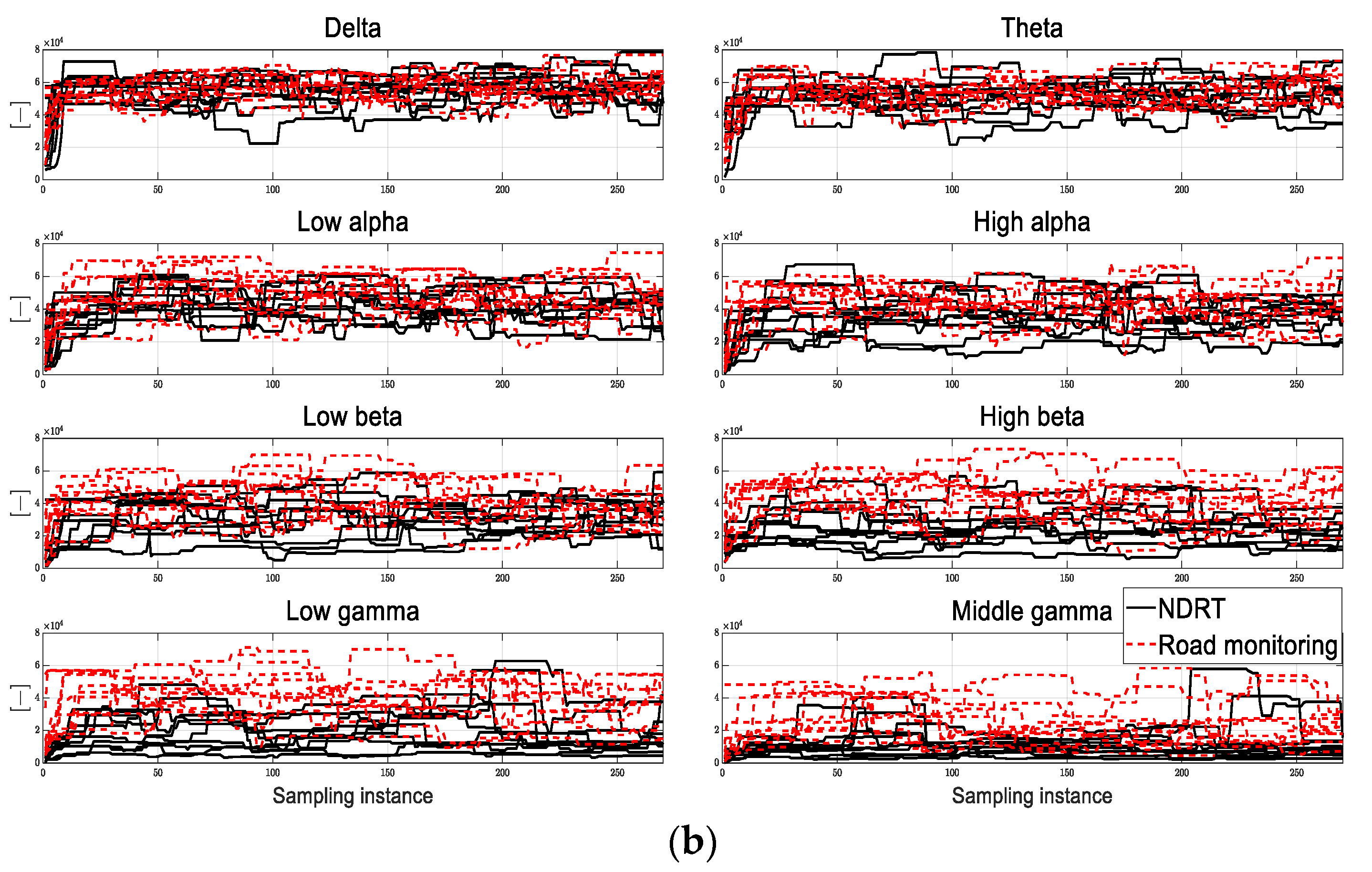
where $x_i$ is the $i$-th EEG data in the sliding window, $\mu$ is the average of the EEG data in the sliding window, $N$ denotes the size of the sliding window, and $x_{max}$ and $x_{min}$ represent the maximum and minimum value of the EEG data in the window, respectively. The calculated values are shown in Figure 5. The applied size of the sliding window is 30.

As shown in Figure 5, it is difficult to confirm the differences between road monitoring and NDRT in the delta, theta, low alpha, and high alpha waves. In contrast, in the low beta, high beta, low gamma, and middle gamma waves, there are significant differences between road monitoring and NDRT. For a quantitative comparison, the average of standard deviation and differences of each EEG signal are calculated, and they are shown in

Table 2. Averages of standard deviations of the EEG in the window.

EEG	Road Monitoring	NDRT
Delta	about 14,983.06	about 14,531.25
Theta	about 14,121.94	about 13,544.83
Low alpha	about 12,370.38	about 10,448.10
High alpha	about 10,750.72	about 8748.90
Low beta	about 10,253.70	about 7384.47
High beta	about 10,872.04	about 6126.67
Low gamma	about 9853.70	about 4515.01
Middle gamma	about 5869.92	about 2733.34

and

Table 3. Averages of differences between minimum and maximum of the EEG in the window.

EEG	Road Monitoring	NDRT
Delta	about 56,554.25	about 55,355.35
Theta	about 53,743.31	about 51,449.74
Low alpha	about 49,196.20	about 42,089.05
High alpha	about 43,577.83	about 35,903.78
Low beta	about 40,718.12	about 30,682.91
High beta	about 42,734.05	about 25,410.22
Low gamma	about 39,355.42	about 18,967.68
Middle gamma	about 24,954.94	about 11,577.92

.

By comparing the calculated averages listed in Table 2 and Table 3, the low beta, high beta, low gamma, and middle gamma waves show the highest differences between road monitoring and NDRT compared to that with the delta, theta, low alpha, and high alpha waves between road monitoring and NDRT. Therefore, it is used to train the standard deviation and differences between the maximum and minimum values in the window for the classification of driver status. To classify driver status, 30,000 pieces of training data are acquired through experimentation. In addition, various ML methods (ANN, RNN, and SVM) are used, and their performances are investigated by comparing the corresponding performance indices to apply proper method to proposed driver status classification. The training processes of the ANN, RNN, and SVM are as follows.

• ANN

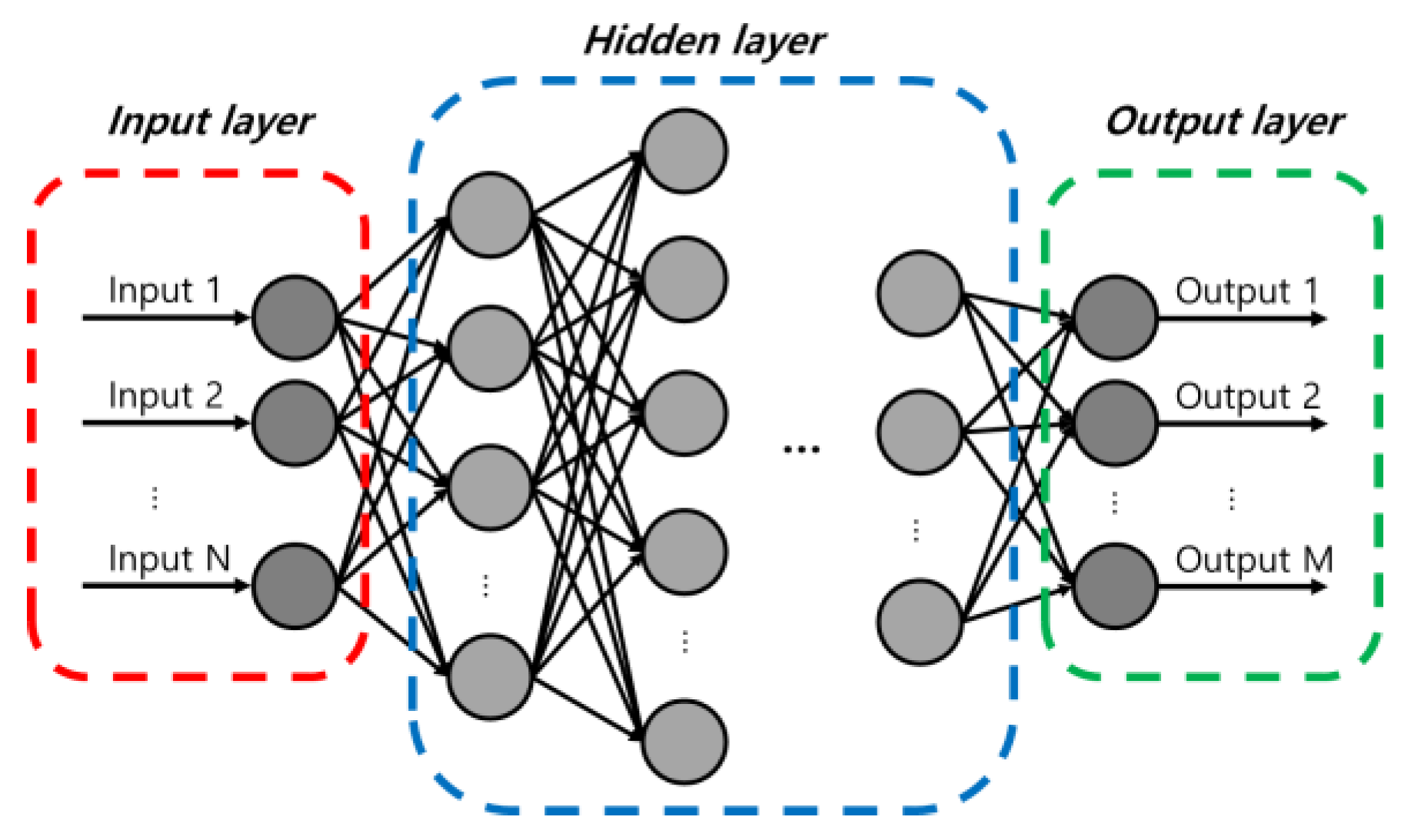
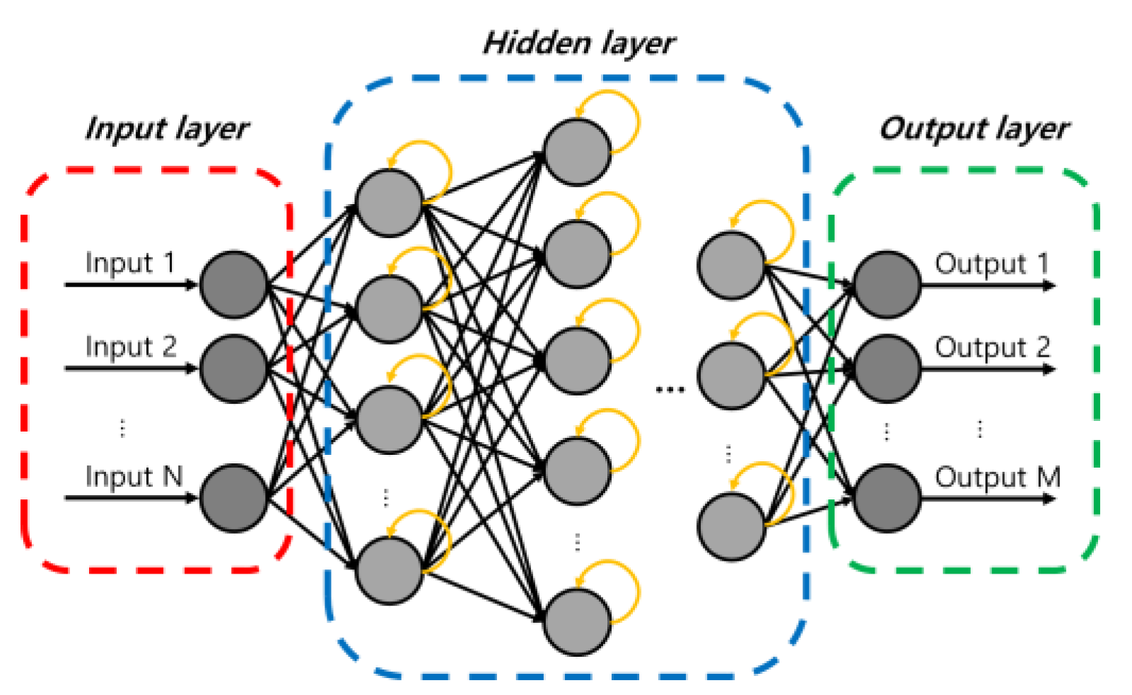
An ANN is a basic neural network structure that includes an input layer, hidden layer, and output layer, as shown in Figure 6. The ANN is designed using the MATHWORKS toolbox(R2019a), deep learning toolboxes, and a pattern recognition method is used to classify the driver status. In this study, 100 hidden layers are applied, and the ratio of training, validation, and test datasets is 8:1:1.

B.

RNN

As shown in Figure 7, an RNN is a neural-network-based learning structure that uses current and past information and predictions on time series or sequences. In this study, an RNN is designed using the MATHWORKS toolbox(R2019a), which is a deep learning toolbox. The dropout technique is used and the Softmax function was adopted as the activation function. Additionally, 100 hidden layers are applied, and the ratio of training, validation, and test data is set as 8:1:1.

C.

SVM

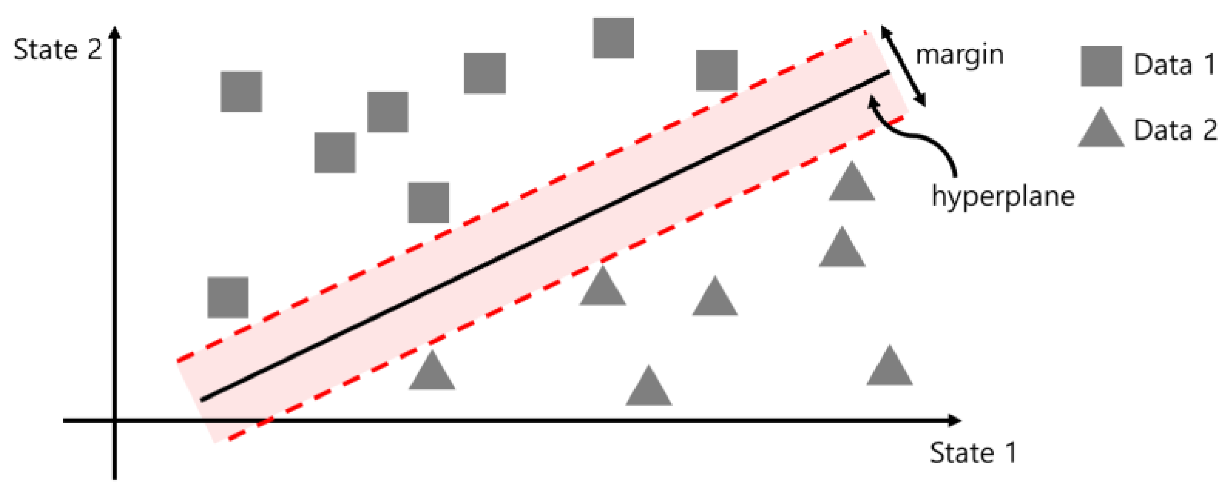
As shown in Figure 8, an SVM is a binary classifier that calculates hyperplanes to optimize the margin between data and hyperplanes. For design, the SVM, MATHWORKS toolbox(R2019a), statistics, and machine learning toolbox are used, and the kernel trick is applied to improve classification performance by applying a kernel radial basis function. In this study, the training and validation datasets are applied in a ratio of 8:2.

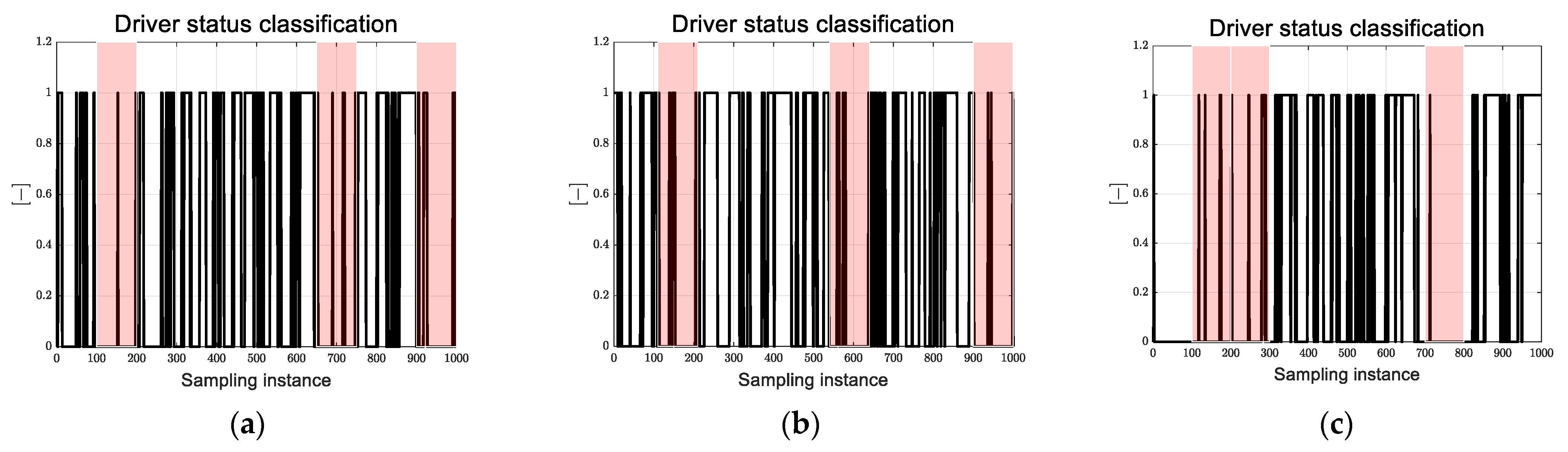
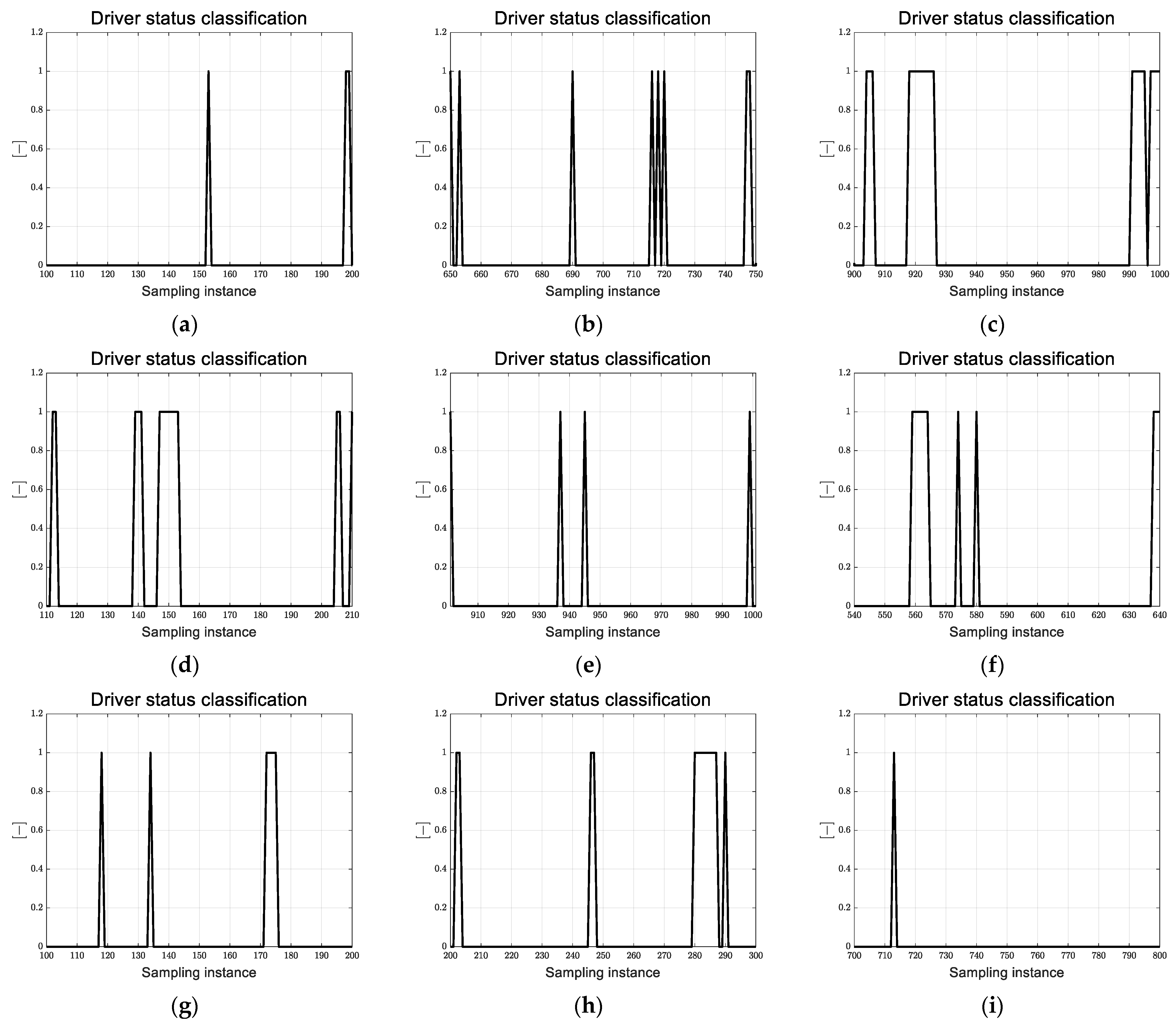
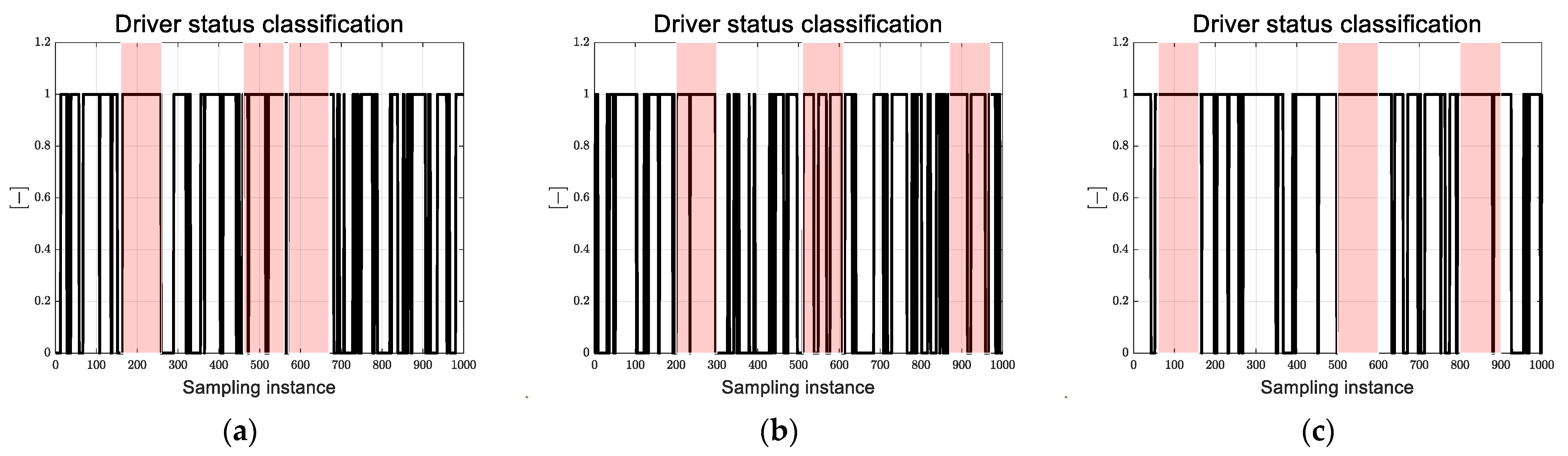
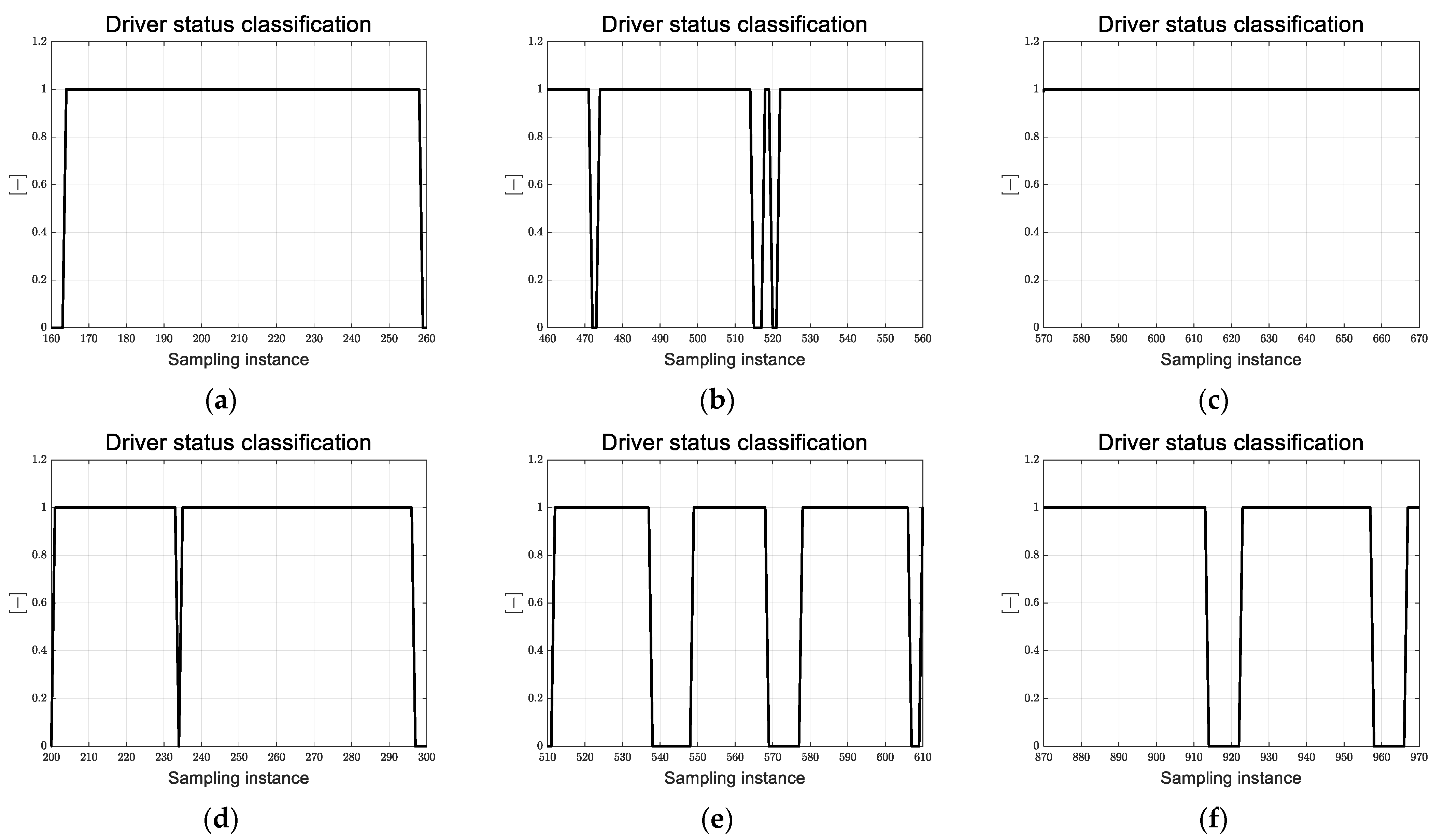
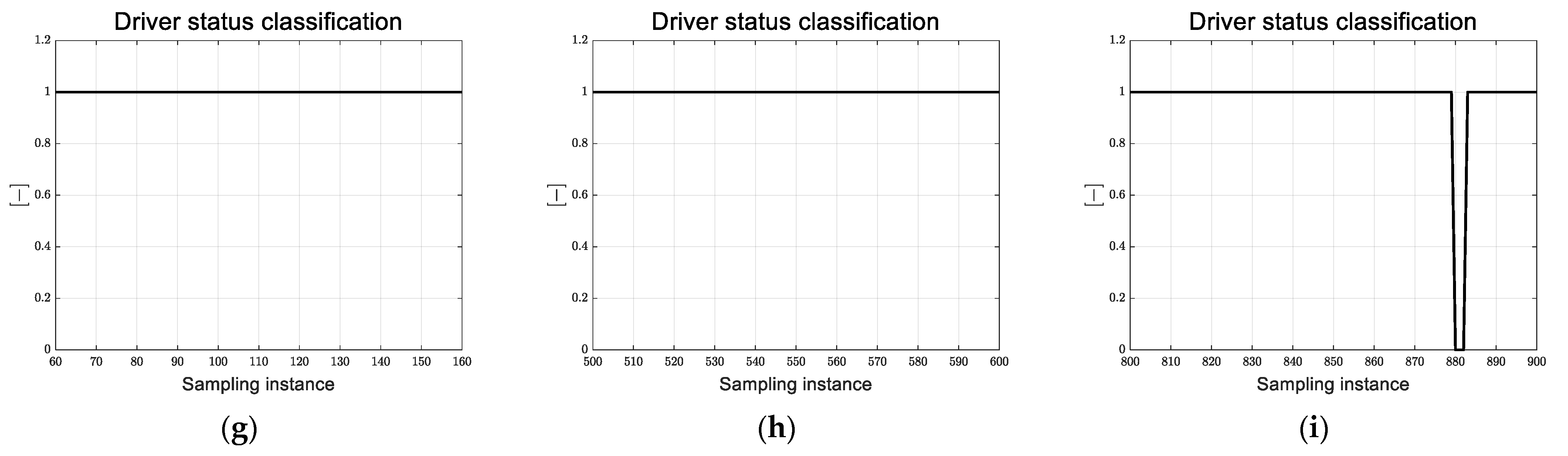
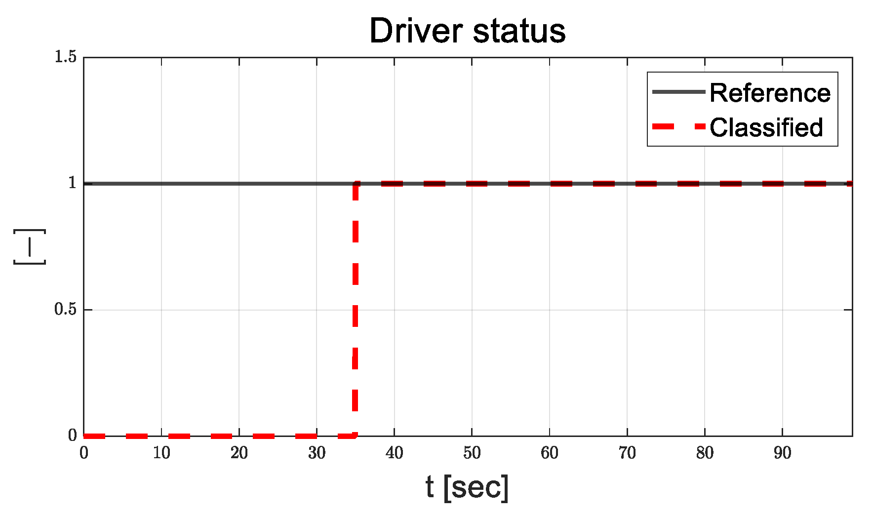
The input data are the extracted feature, which are the standard deviation and differences between the maximum and minimum EEG signals in the window. The outputs are zero or one, indicating road monitoring and NDRT, respectively. The performance of the driver status classification model is evaluated using the Precision, Recall, Accuracy, and F1 scores expressed in Equations (3)–(6).

$$Precision=\frac{TP}{TP+FP}$$

(3)

$$Recall=\frac{TP}{TP+FN}$$

(4)

$$Accuracy=\frac{TP+TN}{TP+FN+FP\_FN}$$

(5)

$$F1 score=2\times \frac{Precision\times Recall}{Precision+Recall}$$

(6)

where TP is true positive, FN is true negative, FP is false positive, and FN is false negative. The performances of ANN, RNN, and SVM are compared in

Table 4. Performance index of driver status classification model.

Performance	ANN	RNN	SVM
Precision	86.5%	62.97%	93.08%
Recall	79.4%	77.01%	89.17%
Accuracy	81.9%	65.86%	91.27%
F1 Score	82.8%	69.29%	91.08%

. Table 4 also presents the results of the driver status classification model.

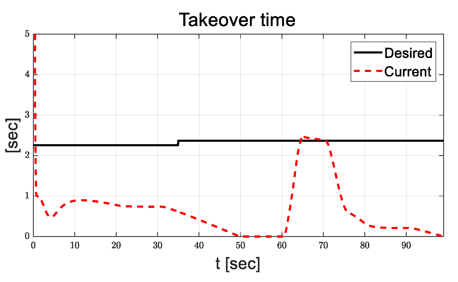
Table 3 lists the performance indices of the ANN, RNN, and SVM. The precisions are 86.5%, 62.97%, and 93.08% for ANN, RNN, and SVM, respectively. The recalls are calculated to be 79.4%, 77.01%, and 89.17%, respectively. The accuracies of the ANN, RNN, and SVM are 81.9%, 65.86%, and 91.27%. The F1 scores are 82.8%, 69.29%, and 91.08%. This evaluation shows that the RNN has the lowest performance and the SVM has the highest performance by comparing the calculated performance index. Because the SVM shows the highest performance, it is suitable for classifying driver status using the EEG in this evaluation. The EEG acquisition equipment constructed in this study can acquire the EEG data in the frequency domain. Because the input data of ML are calculated using the sliding window method by calculating the standard deviation and min/max values and the calculated values, training data, show linearity, it is found that ANN and SVM show relatively higher accuracies than RNN, which shows strength in time series data. Because the proposed feature extraction method can drive spike at noisy EEG data, it is needed to investigate the various method or parameter study to enhance the classification performance. In this study, watching movies is considered as an NDRT. In the future, drivers are expected to be able to perform various tasks in autonomous vehicles. Therefore, it is necessary to acquire and analyze the EEG data affected by various factors that may occur in actual vehicles and to advance the driver status classification model by considering reading, listening to music, and playing mobile games. According to the driver status classified using the EEG, the desired TOT is determined based on [1]. The desired TOT was set to 2.256 s and 2.369 s when the driver conducted road monitoring and NDRT, respectively.

2.2. Desired Clearance Derivation

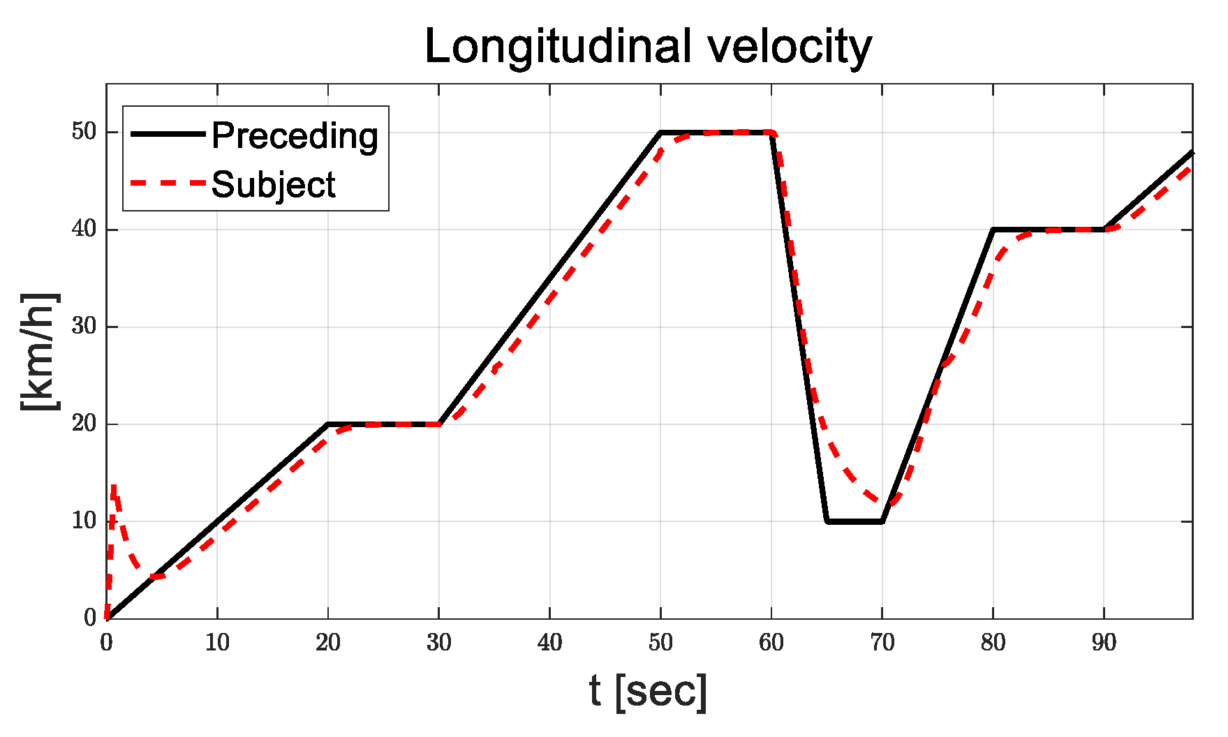
The desired clearance is calculated to ensure the desired TOT or to consider the driving characteristics. The desired TOT is determined as the driver status, as described in Section 2.1. To consider the driving characteristics, a driving experiment was performed using a simulator, and the driving characteristic factor is derived by calculating the time headway. The desired clearance is derived to secure the desired TOT and time headway respectively. First, to ensure the desired TOT, the desired clearance is calculated for three cases based on the longitudinal velocity relationship between the subject and the preceding vehicles in [35]. To ensure a safe takeover, it is assumed that the subject vehicle decelerates to a predetermined deceleration after the takeover request and stops braking deceleration in consideration of the situation in which the driver cannot take over during the desired TOT. Then, the time–velocity plane is designed to calculate the desired clearance ($C_{des,1}$) using the longitudinal velocity of the subject and preceding vehicles by calculating the geometrical area. To prevent collisions, the minimum clearance ($C_{min}$), which is the distance between the subject and preceding vehicles when the subject vehicle stops, is adopted. The derived desired clearance for each case is as follows:

• Case 1. $V_{x,pre}=0\mathrm{k}\mathrm{m}/\mathrm{h}$ (stop condition)

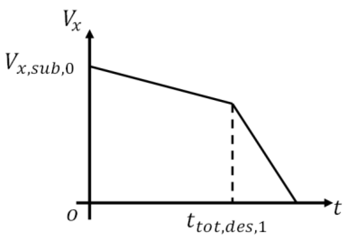
In Case 1, it is assumed that the preceding vehicle stopped, the longitudinal velocity was 0 km/h at the takeover request, and the subject vehicle decelerated. Figure 9 shows an example of the designed time–velocity plane in Case 1.

Here, $V_{x,sub,0}$ is the longitudinal velocity at the takeover request, and $t_{tot,des,1}$ denotes the desired TOT in Case 1. The desired clearance can be expressed by geometrically analyzing the distance while the subject vehicle travels in deceleration, as shown in Equation (7).

$$C_{des,c1}=-\frac{1}{2a_b}{V}_{x,sub,0}^2+\frac{\left(a_b-a_t\right)t_{tot,des,1}}{a_b}{V}_{x,sub,0}+\frac{a_t\left(a_b-a_t\right)t_{tot,des,1}^2}{2a_b}+C_{min}$$

(7)

where $a_b$ and $a_t$ denote the braking and predetermined deceleration, respectively.

B.

Case 2. $V_{x,pre}<V_{x,sub}$

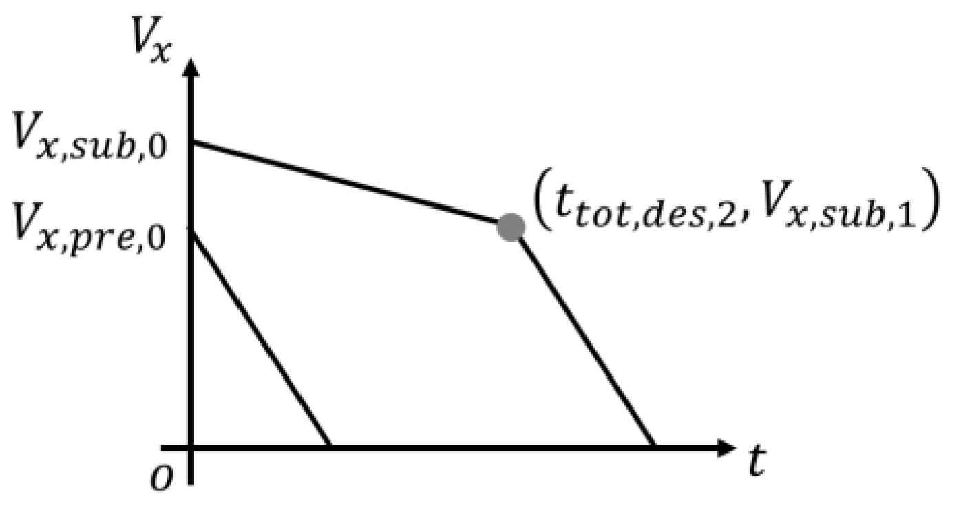
Case 2 represents the situation in which the longitudinal velocity of the subject vehicle is higher than that of the preceding vehicle with braking deceleration at the takeover request. Figure 10 shows an example of the designed time–velocity plane in Case 2.

Here, $V_{x,sub,0}$ and $V_{x,pre,0}$ are the longitudinal velocities of the subject vehicle and preceding vehicle, respectively. At the takeover request, $V_{x,sub,1}$ denotes the longitudinal velocity of the subject vehicle at takeover and $t_{tot,des,2}$ denotes the desired TOT in Case 2. By calculating the clearance between the decelerating subject vehicle and the braking preceding vehicle, the desired clearance can be derived, as expressed in Equation (8).

$$C_{des,c2}=\frac{1}{2}{t}_{tot,des,2}\left(V_{x,sub,0}+V_{x,sub,1}\right)+\frac{V_{x,pre,0}^2-V_{x,sub,1}^2}{2a_b}+C_{min}$$

(8)

C.

Case 3. $V_{x,pre}\ge V_{x,sub}$

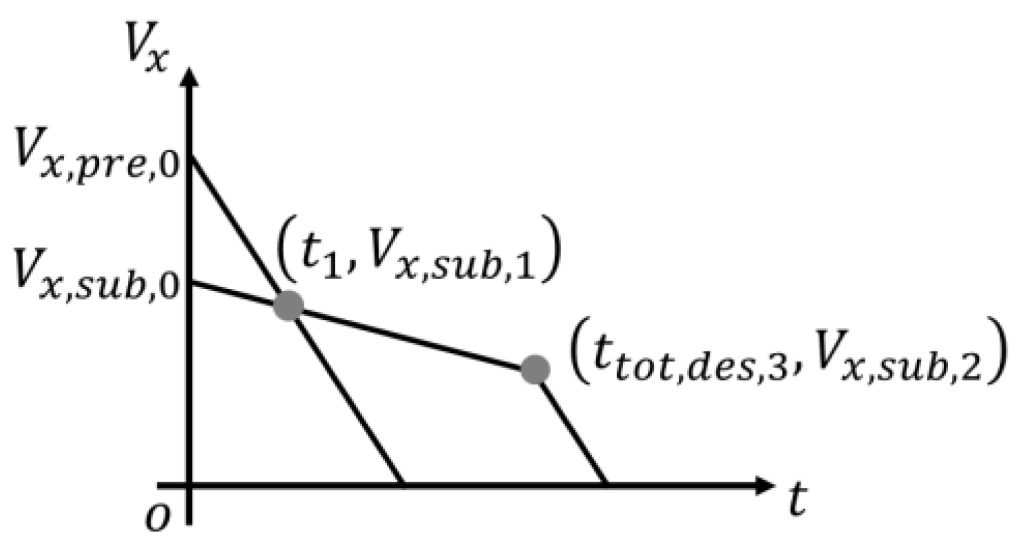
In Case 3, the longitudinal velocity of the preceding vehicle exceeds that of the subject vehicle at the takeover request. It is assumed that the preceding vehicle decelerates to braking deceleration, and the subject vehicle decelerates to predefined deceleration and braking deceleration after takeover. Figure 11 shows an example of the designed time-velocity plane in Case 3.

Where $V_{x,sub,0}$ and $V_{x,pre,0}$ represent the longitudinal velocity of the subject and preceding vehicle, respectively; $t_1$ and $V_{x,sub,1}$ denote the time and longitudinal velocity, respectively, of the subject vehicle when the longitudinal velocities of the subject and preceding vehicles coincide after the takeover request; $t_{tot,des,3}$ is the desired TOT; and $V_{x,sub,2}$ is the longitudinal velocity at takeover. The desired clearance derived by calculating the geometrical area in the time–velocity plane in Case 3 is presented as follows:

$$C_{des,c3}=-\frac{1}{2}{t}_1\left(V_{x,pre,0}-V_{x,sub,0}\right)+\frac{\left(V_{x,sub,1}+V_{x,sub,2}\right)\left(t_{tot,des,3}-t_1\right)}{2}+\frac{V_{x,sub,1}^2+V_{x,sub,2}^2}{2a_b}+C_{min}$$

(9)

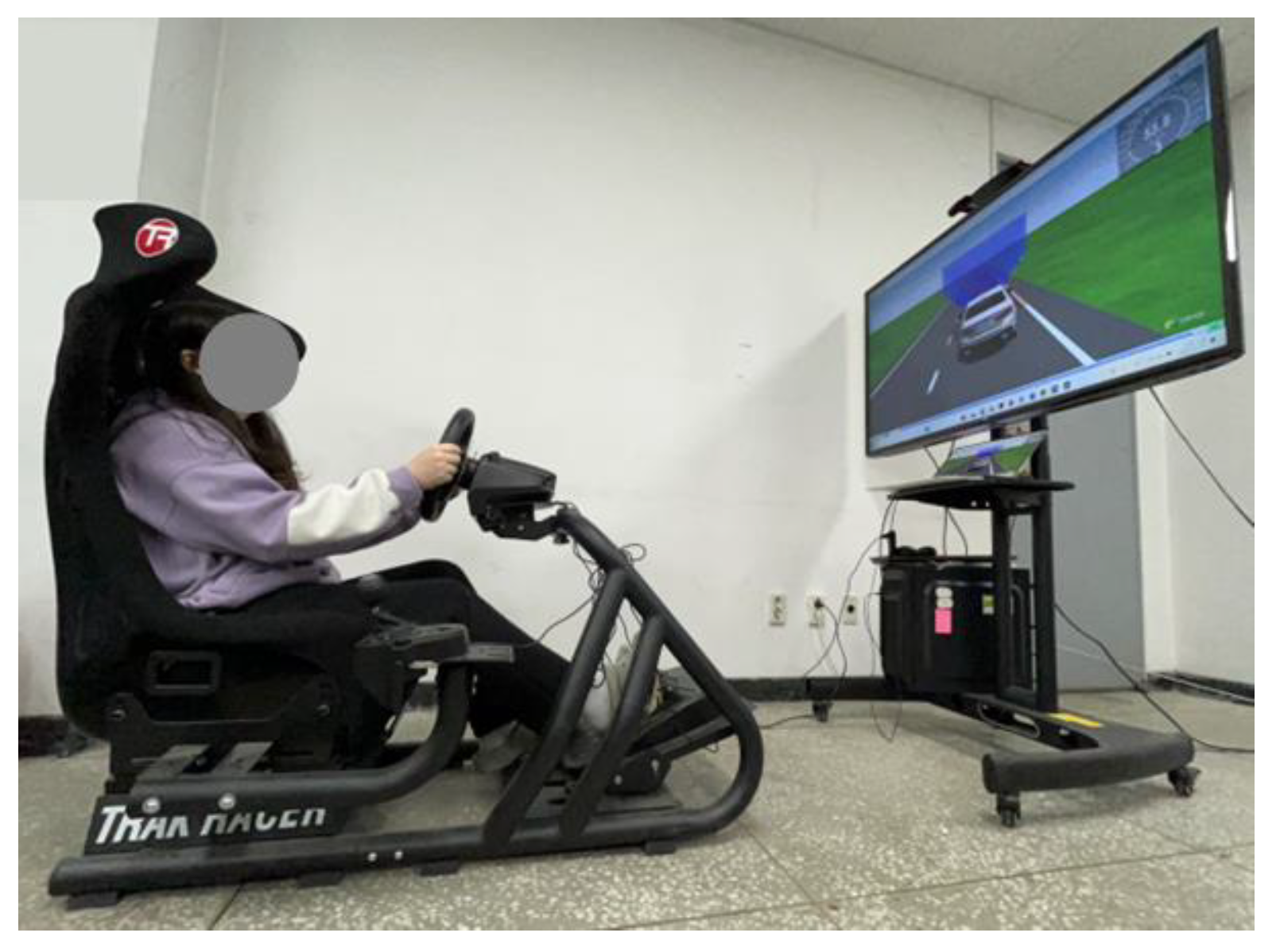
Second, the driving characteristics of each driver are considered to reduce the sense of heterogeneity in autonomous vehicles. To analyze the driving characteristics, an indoor driving experiment using a simulator (Logitech G29) was carried out three times using the CarMaker software to construct a virtual driving environment. Figure 12 shows the environment for the data acquisition of the driving characteristics.

Driving data, including the clearance and longitudinal velocity of the subject and preceding vehicles, were acquired. Using the acquired driving data, the driving characteristics are derived by calculating the time headway, and the desired clearance to secure the driving characteristics is calculated based on the time headway and longitudinal velocity of the subject vehicle, as expressed in Equation (10) and Equation (11), respectively.

$$t_h=\frac{C_{cur}}{V_{x,sub}}$$

(10)

$$C_{des,2}=t_h{V}_{x,sub}$$

(11)

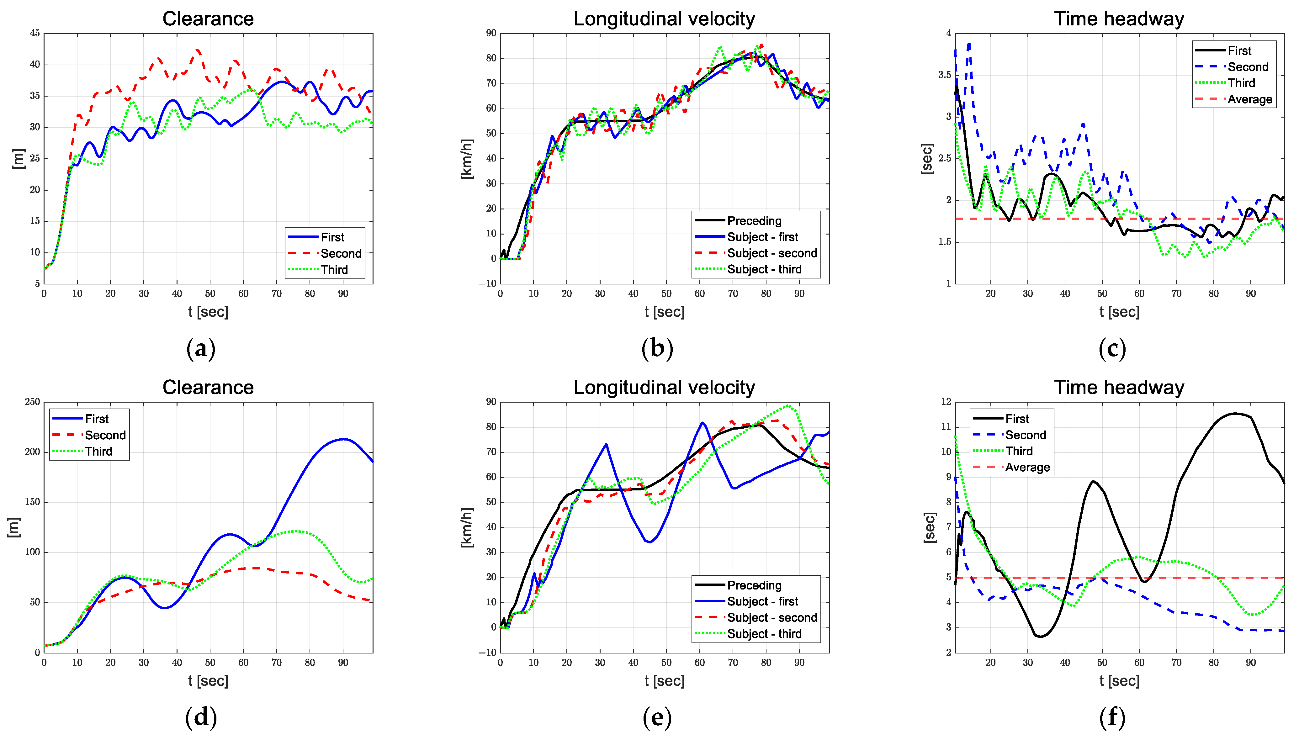
where $C_{cur}$ is the current clearance between the subject and preceding vehicles and $C_{des,2}$ is the desired clearance to consider the driver characteristics. Figure 13 shows the representative acquired driving data of the drivers who were familiar (Driver 3) and unfamiliar (Driver 9) with driving.

For drivers who are familiar with driving, such as Driver 3, driving characteristics can be confirmed by the propensity of each driver, such as maintaining constant clearance or increasing clearance proportionally with longitudinal velocity. For drivers who are not familiar with driving, such as Driver 9, it is difficult to analyze a certain propensity.

Table 5. Calculated time headway of each driver.

Driver	Time Headway (Average)
Driver 1	1.4171 s
Driver 2	1.4551 s
Driver 3 (data are in Figure 10)	1.7825 s
Driver 4	2.1465 s
Driver 5	1.4202 s
Driver 6	1.5684 s
Driver 7	1.5671 s
Driver 8	2.6198 s
Driver 9 (data are in Figure 10)	4.9874 s
Driver 10	2.1954 s

lists the calculated average time headway of each driver.

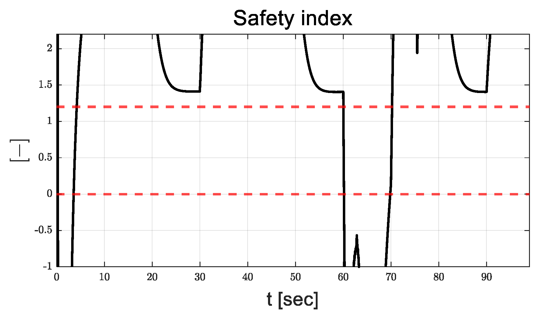
2.3. Safety-Index-Based Desired Clearance Transition

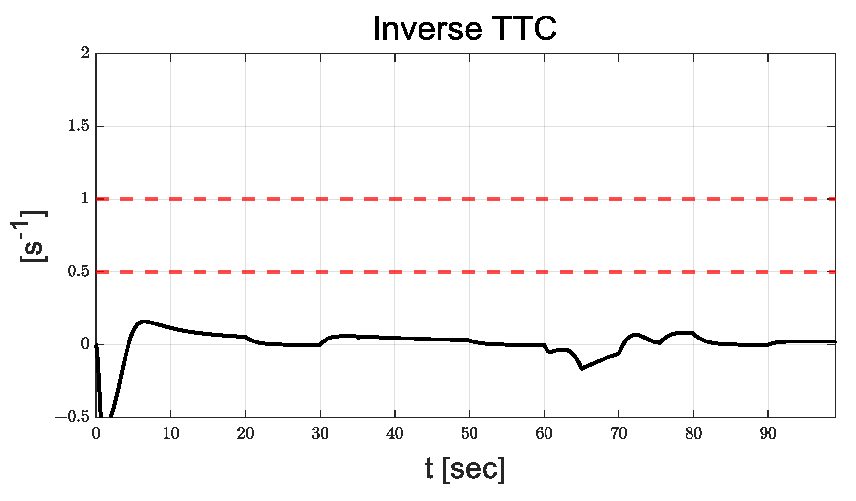
In this research, a safety index is designed to determine the driving situation and includes safety, warning, and emergency, with inverse time-to-collision (TTC) based on [36,37,38]. The safety index is expressed by Equation (12) according to the current vehicle state, braking distance, and warning distance.

$$I_{safety}=\frac{C_{cur}-d_{br}}{d_w-b_{br}}$$

(12)

where $C_{cur}$ denotes the current clearance between the subject and preceding vehicles, $d_{br}$ denotes the braking distance, and $d_w$ denotes the warning distance. The braking and warning distances indicate that if $C_{cur}$ exceeds $d_{br}$ or $d_w$, the driving situation is safe, whereas when $C_{cur}$ is below $d_{br}$, it is dangerous. The braking and warning distances are calculated using Equation (13) and Equation (14), respectively.

$$d_w=V_{rel}{\tau }_{sys}+f(\mu )\left(\frac{V_{x,sub}^2-{\left(V_{x,sub}-V_{rel}\right)}^2}{2a_{ax,max}}\right)$$

(13)

$$d_{br}=V_{rel}{\tau }_{sys}+f(\mu )\left(\frac{V_{x,sub}^2-{\left(V_{x,sub}-V_{rel}\right)}^2}{2a_{x,max}}\right)+V_{sub}{\tau }_{human}$$

(14)

where $V_{rel}$ is relative longitudinal velocity between subject and preceding vehicles, ${\tau }_{sys}$ is system time delay, ${\tau }_{human}$ is human time delay, and $a_{x,max}$ is maximum of longitudinal deceleration on normal road. The inverse TTC is expressed by Equation (15).

$${TTC}^{-1}=\frac{V_{x,pre}-V_{x,sub}}{C_{cur}}$$

(15)

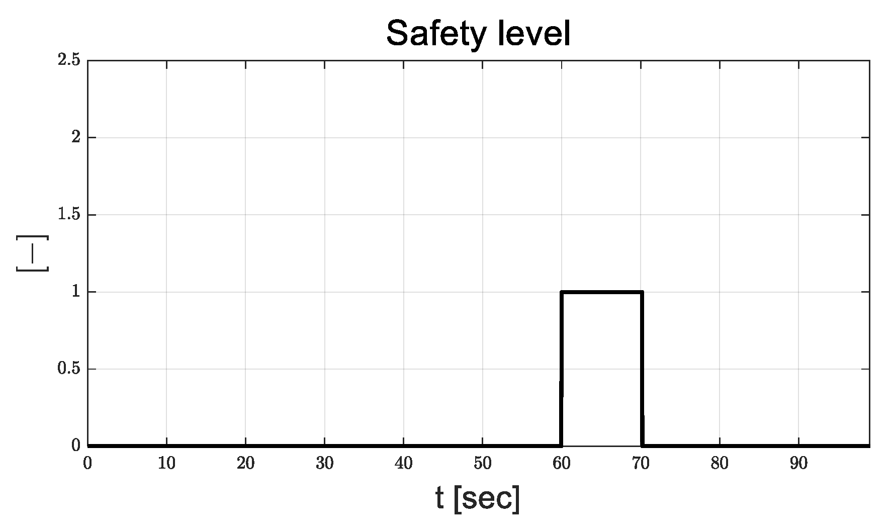
According to the safety index and inverse TTC, safety level, safety, warning, and emergency are determined as follows:

• Inequality condition for safety level

$$I_{sfaety}\ge I_{safety,th,1}\mathrm{a}\mathrm{n}\mathrm{d}{TTC}^{-1}\le {TTC}_{th,1}^{-1}$$

(16)

B.

Inequality condition for warning level

$$I_{sfaety}<I_{safety,th,1}\mathrm{o}\mathrm{r}{TTC}^{-1}>{TTC}_{th,1}^{-1}$$

(17)

C.

Inequality condition for emergency level

$$I_{sfaety}\le I_{safety,th,2}\mathrm{a}\mathrm{n}\mathrm{d}{TTC}^{-1}>{TTC}_{th,2}^{-1}$$

(18)

When the current driving situation is determined to be safe, the safety level is zero, and the desired clearance is determined based on the driving characteristics, which are analyzed experimentally. When the current driving situation is determined as a warning or emergency, indicating a safety level of 1 or 2, respectively, the desired clearance is calculated based on the desired TOT described in Section 2.2.

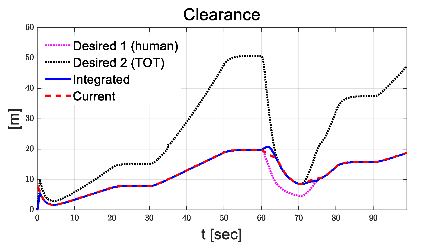
The integrated desired clearance is determined based on safety index and calculated using the third-order polynomial function ($\alpha$) in transient time.

$$C_{des,int}=(1-\alpha )C_{des,1}+\alpha C_{des,2}$$

(19)

where $C_{des,int}$ is the integrated desired clearance, $C_{des,1}$ is the desired clearance considering the driver characteristics, and $C_{des,2}$ represents the desired clearance ensuring the desired TOT, which is determined by the driver status.

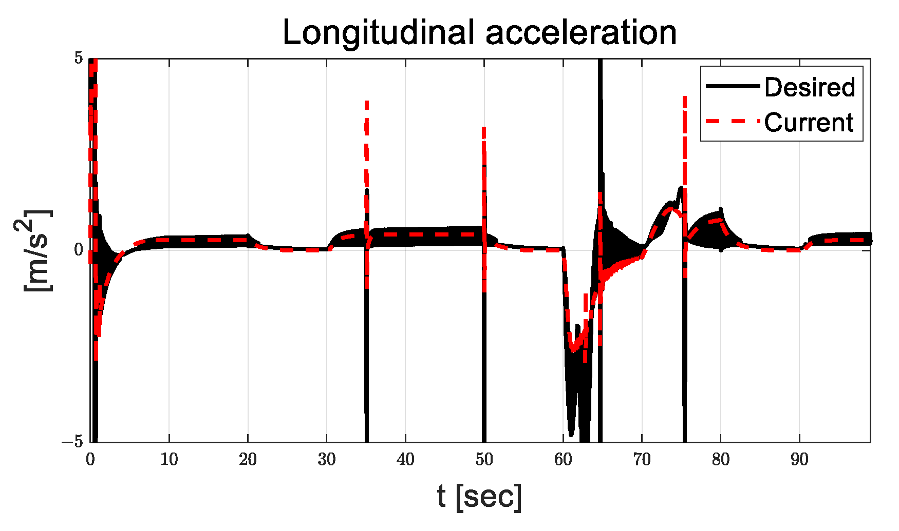
2.4. SMC-Based Longitudinal Control Algorithm

The SMC is designed to track the desired clearance by calculating the desired longitudinal acceleration under Lyapunov stability conditions. To design the SMC, the control error is defined using the desired and current clearances, and the control input is derived based on the Lyapunov stability conditions. The control errors are defined using the clearance and longitudinal velocity in Equation (20) and Equation (21), respectively.

$$e_1=C_{des,int}-C_{cur}$$

(20)

$${\dot{e}}_1=e_2={\dot{C}}_{des,int}-\left(V_{x,pre}-V_{x,sub}\right)$$

(21)

The sliding surface is defined as follows.

$$\sigma =e_2+\lambda e_1\mathrm{where}\lambda >0.$$

(22)

In this paper, the sliding surface is designed using a linear combination of control errors simply, however, it is considered an advancement in the design process to reduce the chattering phenomenon. To calculate the control input that ensures Lyapunov stability, a cost function is designed based on the Lyapunov candidate function, as expressed in Equation (23).

$$J=\frac{1}{2}{\sigma }^2$$

(23)

Based on the definition of a sliding surface in Equation (22), the time derivative of the designed cost function can be obtained using Equation (24).

$$\dot{J}=\sigma \dot{\sigma }=\sigma \left({\ddot{C}}_{des,int}-\left(a_{x,pre}-a_{x,sub}\right)+\lambda e_2\right)$$

(24)

The disturbance boundary and injection term are defined in Equations (25) and (26), the time derivative of the cost function can be rewritten as Equation (27).

$$\left|{\ddot{C}}_{des,int}-a_{x,pre}+\lambda e_2\right|\le L_b$$

(25)

$$a_{x,sub}=\nu \mathrm{w}\mathrm{h}\mathrm{e}\mathrm{r}\mathrm{e}\nu =-\rho sign(\sigma ).$$

(26)

$$\dot{J}\le -\left|\sigma \right|\left(\rho -L_b\right)$$

(27)

Using finite-time convergence conditions, the time derivative of the cost function can be described as Equation (28).

$$\dot{J}\le -\alpha J^{\frac{1}{2}}=-\alpha \frac{\left|\sigma \right|}{\sqrt{2}}$$

(28)

where $\alpha$ denotes decay rate of Lyapunov function. Then, by subtracting Equations (27) and (28), the magnitude of the injection term can be derived as:

$$\rho =L_b+\frac{\alpha }{\sqrt{2}}$$

(29)

Therefore, the control input is calculated as the desired longitudinal acceleration by subtracting Equations (26) and (29), which are expressed as Equation (30).

$$a_{x,des}=a_{x,sub}=-\left(L_b+\frac{\alpha }{\sqrt{2}}\right)sign(\sigma )$$

(30)

To reduce the chattering phenomenon in the SMC, a sigmoid function is utilized as a sign function, as expressed in Equation (31).

$$S(\sigma ,m)=\frac{m\sigma }{1+m\left|\sigma \right|}$$

(31)

where $m$ denotes the gradient of the sigmoid function determined by trial and error.

2.5. Stability Analysis of the SMC

In this section, the stability analysis is performed based on Lyapunov direct method. By subtracting Equations (27) and (29), the time derivative of cost function can be satisfied inequality condition as Equation (32).

$$\dot{J}\le -\left|\sigma \right|\left(\left(L_b+\frac{\alpha }{\sqrt{2}}\right)-L_b\right)=-\frac{\alpha }{\sqrt{2}}\left|\sigma \right|$$

(32)

$\alpha$ is designed as positive value, and the time derivative of cost function is always negative, excepting when $\sigma$ is 0. Since the cost function $J$ is a positive definite and $\dot{J}$ is a semi-negative definite, the SMC-based longitudinal controller satisfies the Lyapunov stability condition.

3. Performance Evaluation

3.1. Driver Status Classification Model Evaluation in Real Time

In this experiment, because the SVM showed greatest classification performance in Section 2.1, the SVM-based driver status classification model was evaluated using the MATLAB(R2019a) and EEG data acquisition equipment in real time. The SVM was trained to classify the driver status using the standard deviation and differences between the maximum and minimum values in the windows of low beta, high beta, low gamma, and high gamma waves. The output of the SVM was set to 0 or 1, indicating that the driver status is road monitoring and NDRT, respectively. Three drivers (two males and one female) from the previous experiment volunteered to carry on the experiment for 1000 sampling instances. The performance of the driver status classification model is verified using the accuracy in Equation (5). Figure 14 shows the real time evaluation results for each driver, and Figure 15 shows the highest accuracy results for 100 sampling instances during road monitoring.

In this situation, three drivers conducted road monitoring for 1000 sampling instances. The reference driver status is 0, which indicates road monitoring. As shown in Figure 14, the performance of the proposed driver status classification model over the entire experiment is relatively low. However, during a specific set of 100 sampling instances, it shows a relatively high performance in the red-shaded box. To analyze the performance of the real time classification model, the accuracy is calculated using the EEG data after 30 sampling instances, considering the application of the sliding window method for feature extraction. The accuracies for Driver 1 are 98%, 93%, and 80%. The accuracies for Driver 2 are 86%, 97%, and 90%, and those for Driver 3 are 95%, 88%, and 99%. The results of the real-time evaluation of the NDRT are shown in Figure 16 and Figure 17.

In this situation, the driver conducted an NDRT, watching a movie, for 1000 sampling instances, and the reference for classification is 0. As the driver performed road monitoring, they showed a relatively low accuracy for the entire experiment; however, they had a relatively high accuracy for 100 sampling instances, as shown in the red-shaded box in Figure 16. The accuracies for Driver 1 are 95%, 94%, and 100%, and those for Driver 2 are 95%, 76%, and 83%. The accuracies for Driver 3 are 100%, 100%, and 98%. In this research, the EEG data are acquired when the driver is focusing on the specific task (i.e., road monitoring or watching a movie), and factors that can affect the driver EEG signal that may occur during the experiment (e.g., workload, emotion, noise) are not considered. Since the EEG is affected by the subject’s condition and experiment [39,40], it is expected that the proposed EEG-based driver status classification model can be applied to an actual system if the EEG is analyzed considering various effects in the future.

3.2. Integrated Longitudinal Control Algorithm Evaluation

The performance of the proposed algorithm was evaluated via the MATLAB/Simulink R2019a and CarMaker software 8.1.1 in a car-following scenario. The longitudinal velocity of the preceding vehicle varied up to 50 km/h, and the subject vehicle calculated the desired clearance between the subject and preceding vehicles, considering the driver status and driving characteristics. The driver status was classified based on the SVM-based driver status classification model using the acquired EEG data. The desired clearance was calculated to ensure the desired TOT and driving characteristics. The desired TOT was determined based on the classified driver status, and the driving characteristic factor was applied using the time headway derived from the experiment. To determine the integrated desired clearance, the safety level was determined by calculating the safety index and inverse TTC using the vehicle states. The SMC was utilized to track the integrated desired clearance by computing the desired longitudinal acceleration.

Table 6. Vehicle specifications for the performance evaluation.

Division	Value
Length between front wheel axle and mass center	1.47 m
Length between rear wheel axle and mass center	1.5 m
Track width (front/rear)	0.831 m/0.85 m
Vehicle mass	2108 kg
Moment of inertia of vehicle	3170.6 kg·m2

and

Table 7. Control and threshold parameters for the performance evaluation.

Division	Value
Decay rate of sliding surface ($\lambda$)	7
Decay rate of Lyapunov function ($\alpha$)	6
Gradient of sigmoid function ($m$)	0.1
Threshold for safety index ($I_{safety,th,1}/I_{safety,th,2}$)	0/1
Threshold for inverse TTC (${TTC}_{th,1}^{-1}/{TTC}_{th,2}^{-1}$)	0.5/1

present the vehicle specifications and tuning parameters used for performance evaluation, respectively.

The desired TOT when driver conducts road monitoring and NDRT are 2.256 s and 2.369 s, respectively, and the time headway is 1.4171 s for Driver 1. The EEG data when the driver status is NDRT are used as described in Section 2.1. Figure 18, Figure 19, Figure 20, Figure 21, Figure 22, Figure 23, Figure 24 and Figure 25 present the performance evaluation results.

Figure 18 shows the longitudinal velocity, and the longitudinal velocity of the subject vehicle drives similar to the preceding vehicle. Figure 19 shows the desired and current clearance between the subject and preceding vehicle. Desired Clearance 1 is calculated based on the driving characteristics, and Desired Clearance 2 indicates the calculated clearance, ensuring the desired TOT. The integrated desired clearance was determined between Desired Clearances 1 and 2 in transient times of approximately 60–65 s and 70–75 s. The subject vehicle tracks the integrated desired clearance reasonably because the maximum clearance error is approximately 2.5 m and the standard deviation of the clearance error is 0.5842 m. The driver status was classified as 1 according to the driver status being set to NDRT, as shown in Figure 20. A classification delay occurs for approximately 30 s by using the sliding window method, because a window size of 30 was adopted. Figure 21 shows the safety index, which has a value above the threshold before 60 s and after 70 s and a value between or below the two thresholds at 60–70 s. The inverse TTC has a value below the two thresholds, as shown in Figure 22. As the safety index and reverse TTC are calculated as described above, the safety index was determined to be 1, indicating a warning level between 60–70 s. The desired longitudinal acceleration from the SMC and current longitudinal acceleration of the subject vehicle are shown in Figure 24. It can be confirmed that the longitudinal acceleration is calculated as a negative value as the safety level increases from safe (0) to warning (1) level and the desired clearance increased from 60–70 s. Since the chattering phenomenon of the SMC occurred significantly, the advancement of the SMC and lower-level controller, the PI-based pedal controller, is considered for the future. Figure 25 illustrates the desired TOT and current TOT, and it can be seen that the desired TOT is secured from 60–70 s, where the safety level is determined as warning level. If the control error is higher than 2 m, it can lead to a relatively dangerous situation. This is analyzed to be influenced by the chattering phenomenon of the SMC and the PI-based pedal controller and the safety index that responds to the vehicle status sensitivity. Therefore, we plan to consider the development of an advanced SMC and lower-level controller and the safety index.

4. Conclusions

The driver’s status can affect their perception and response ability. However, the development of an autonomous driving system considering the driver status has been insufficiently carried out. Therefore, the DMSs and autonomous control algorithm considering driver status are required to ensure safety and stability in autonomous vehicles at SAE Level 3. In this study, to monitor the driver status, the EEG-based driver status classification model was proposed to categorize the driver status as road monitoring or NDRT. Then, the desired TOT was determined based on the classified driver status. The safety index and inverse TTC were calculated using vehicle states to determine the safety levels as safe, warning, and emergency. In order to secure longitudinal safety, the SMC-based longitudinal control algorithm was designed to track the desired TOT and driving characteristics considering the safety index. The performance of the proposed algorithm was evaluated in a car-following scenario using the MATLAB/Simulink R2019a and CarMaker software 8.1.1.

In this study, we investigated the possibility of using the EEG-based driver status monitoring by excluding various external factors during EEG data acquisition. In the future, we aim to acquire the EEG data by considering various outdoor driving factors (for example, car sickness, traffic conditions, and noise), and it is also necessary to analyze the EEG when driver status is converted in transient time. In addition, to advance the proposed driver status classification model, the driver status was classified into various statuses, including conversations with passengers, reading books, listening to music, texting, and playing mobile games. Since the performance of the SMC and the lower-level controller can affect control performance, such as the chattering phenomenon, it is planned to advance the controller by applying a second-order SMC and a reasonable switching method for lower-level controllers. Moreover, a lateral safety feature such as obstacle avoidance is also valuable to ensure driver safety in autonomous vehicles. Therefore, to advance the proposed takeover system, it is necessary to develop and analyze the lateral response of drivers and vehicles in the future.

This study presents the possibility of using the EEG for DMSs in autonomous mobilities by proposing the driver status classification model with driver EEG. Moreover, the proposed takeover and longitudinal control algorithm is expected to be utilized as a DMSs by ensuring driver safety for commercialization over SAE Level 3 autonomous vehicles. This study presents the possibility of using the EEG for DMSs in autonomous vehicles by proposing a driver status classification model using the driver EEG. Moreover, the proposed takeover and longitudinal control algorithm is expected to be utilized as a DMSs to ensure driver safety for commercialization over SAE Level 3 autonomous mobilities.