Non-Fragile Prescribed Performance Control of Robotic System without Function Approximation

Abstract

In order to address the fragility issues associated with the current prescribed performance control (PPC) strategy and ensure both transient and steady-state performance of the tracking error, a non-fragility prescribed performance control scheme is proposed. A non-fragile prescribed performance control method for robotic systems with model uncertainties and unknown disturbances is developed. This method not only addresses the inherent vulnerability defects of the existing prescribed performance control but also effectively reduces the computational complexity of the controller. Firstly, addressing the fragility issues of existing PPC, a new non-fragile prescribed performance control strategy is proposed. To address the fragile issue with the current PPC, the shift function is employed to handle the tracking error. Based on the non-fragile PPC mentioned above, a new prescribed performance controller is designed without the requirement for approximation or estimation. This effectively reduces the complexity of controller design. At last, the feasibility of achieving non-fragile prescribed performance is verified through stability analysis, and the superiority of the designed controller is confirmed through simulation comparisons. The results show that the designed controller effectively resolves the control singularity issue arising from the inherent limitations of the PPC.

1. Introduction

Robot systems have great potential for development in industrial applications. The inherent nonlinear, strong coupling, and uncertain dynamic characteristics of robot systems pose significant challenges for controller design [1,2,3]. As a result, the design of robot control systems has become an important area of research. The primary objective of robot system control is to ensure that the control system can achieve ideal transient performance, high-precision tracking performance, and fast response capability, as well as exhibit high robustness to handle unknown dynamics.

In order to ensure the ideal transient performance of the control system, several control strategies based on prescribed performance control have been proposed [4,5,6,7,8]. In reference [4], a non-singular fixed-time terminal sliding mode prescribed performance control strategy is proposed. This strategy combines terminal sliding mode control with PPC for the robot manipulator system, considering external disturbances and parameter uncertainties. The designed controller can offer faster transient performance and higher steady-state tracking accuracy. Based on this, the controller is further extended in reference [5]. A fixed-time fault-tolerant PPC is designed by integrating fault-tolerant control with PPC to tackle the tracking control issue in the event of actuator failure. This design improvement enhances both the transient and steady-state accuracy and increases the robustness of the control method. In reference [6], the combination of neural networks and observers is employed to achieve prescribed performance control of the robot system for various types of actuator faults. This approach ensures both transient and steady-state performance of the system. In reference [7], the fixed-time sliding mode control is combined with PPC, and a radial basis neural network is employed to address the lumped uncertainty of the system. A method for controlling the performance of a robot system based on a fixed-time neural network is proposed. This method achieves the prescribed performance within a fixed time and effectively addresses the issue of synovial buffeting. Different from the aforementioned PPC control strategies that all need to meet certain initial conditions, reference [8] converts the tracking error into an intermediate variable by designing certain correlation functions and imposes new performance constraints on these intermediate variables. In this way, the dependence on initial conditions is resolved, the limitations of existing PPC related to initial conditions are eliminated, and the global tracking control effect is achieved without considering initial conditions. In reference [9], PPC is combined with robust adaptive control and applied to the manual 3T1R parallel robot to ensure the system meets steady-state and transient tracking requirements during high-speed grabbing. In reference [10], a performance-based neural adaptive control scheme for manipulators is proposed. The designed controller has minimal measurement and hardware requirements for manipulator trajectory tracking in industrial automation. In reference [11], a coordinated tracking control strategy for tractor-towing systems is proposed. Through the effective application of PPC technology, the performance requirements of the controller are guaranteed.

Another concern is the challenge of high-precision tracking in the presence of unknowns and external disturbances. In recent years, the control method based on disturbance observer has become one of the most effective methods to address the impact of disturbances [12,13,14,15]. The fundamental concept of this method involves designing a disturbance observer to estimate and compensate for unknown disturbances. The control law is then designed based on the estimated information to ensure system stability. However, constructing the general observer requires system information. The observer-based control method is only effective for systems that are partially unknown. Therefore, the global approximator based on fuzzy system/neural network approximation is applied to the controller with completely unknown system dynamics [16,17,18]. The fuzzy/neural approximator requires online learning parameters for training [19,20,21] and additional design based on Lyapunov’s adaptive law to adjust its weight. To enhance tracking accuracy, it is essential to have adequate online learning parameters and adaptive parameters. However, the real-time performance of the robot control system is a crucial factor that needs to be taken into account during actual operation. Excessive online learning parameters and adaptive parameters can result in poor real-time performance of the controller. This can significantly increase the amount of calculations, which is not conducive to effectively controlling the robot system.

Despite the attainment of the aforementioned results, there are still unnoticed problems. Specifically, the current prescribed performance control strategy [4,5,6,7,8] still has issues with fragility. The sudden external interference in the robot system can cause fluctuations in the tracking error. When external interference occurs, the system is affected, resulting in the tracking error fluctuating over time. If the error fluctuation caused by interference is too large, it may lead to the error reaching or directly crossing the set performance constraint, which can result in control singularity. This is about the fragility issues of PPC [22,23]. According to the analysis above, the current prescribed performance control scheme demonstrates a clear fragility to sudden system interference. Furthermore, the current control strategy, based on fuzzy systems and neural approximation, has proven to be effective in addressing the uncertainties in the dynamics of the controlled system model and guaranteeing the desired robust performance. However, it requires a specific number of online learning parameters for the fuzzy/neural approximator. The impact of these online learning parameters and adaptive parameters on the real-time performance and computational complexity of the controller is evident. Therefore, it is necessary to further reduce the number of online learning parameters and adaptive parameters in order to ensure the real-time performance of the control system. Driven by the above discussion and inspired by reference [8], a new non-fragile PPC scheme is designed to ensure that the tracking error can exhibit ideal transient and steady-state performance even in the presence of interference. The controller does not involve function approximation or adaptive parameters. The main contributions are summarized as follows:

(1)

Unlike existing PPC strategies, control singularity occurs when bursts of interference cause tracking errors to be close to performance boundaries. In this paper, a non-fragility control strategy with a shift function is designed. When the error is close to the boundary, the shift function can adjust the error based on its own characteristics. Therefore, the aforementioned issues are avoided, and the tracking error can meet the prescribed performance.

(2)

Different from the existing methods that rely on adaptive laws, neural networks, or fuzzy logic systems to handle the nonlinear uncertainty of the system [24,25,26], the proposed approach does not require similar approximate constructions. This approach avoids the high complexity of controller design and offers better real-time performance.

(3)

The controller designed in this paper does not contain any prior knowledge of system nonlinearity, nor does it include the relevant boundary functions. This approach relaxes the key assumptions in the relevant literature [4,5]. This enhances the suitability of the controller and its robustness to system uncertainties.

The rest of this article is summarized as follows. The problem description is proposed in Section 2, and the controller is developed in Section 3. In Section 4, we present the simulation results, which confirm the effectiveness and superiority of the method. The conclusion is finally presented Section 5.

2. Problem Statement

In this section, the dynamic modeling of robots under external interference is first discussed, and some necessary properties and assumptions are provided. To address the control singularity issue, where the tracking error might exceed performance limits during perturbations, a non-fragile PPC strategy is developed by introducing a shift function. On this basis, the design process and stability proofs of the controller will be presented in the following chapters.

2.1. Robot Dynamics

The dynamics of an n-DOF rigid robot manipulator in joint space can be described as follows [6]:

$$M\left(q\right)\ddot{q}+C(q,\dot{q})\dot{q}+G\left(q\right)=\tau \left(t\right)-d\left(t\right)$$

(1)

where $q\in R^n$, $M\left(q\right)\in R^{n\times n}$, $C(q,\dot{q})\in R^{n\times n}$, $G\left(q\right)\in R^n$, $\tau \left(t\right)\in R^n$, $d\left(t\right)\in R^n$ represent joint angular displacement, robot inertia matrix, centrifugal force and Coriolis force matrix, gravity term, control torque, and unknown disturbance, respectively.

Considering the uncertainty of Equation (1) in the actual model, we have obtained the following dynamic model:

$$M\left(q\right)\ddot{q}+C(q,\dot{q})\dot{q}+G\left(q\right)=\tau \left(t\right)+\Delta$$

(2)

where $\Delta$ represents the concentrated disturbance, which includes model uncertainty and unknown external disturbances. In this study, the actual joint angular displacement and joint angular velocity are supposed as measurable and bounded. The rest of the permits are completely unknown, but the aim is to meet the following properties and assumptions:

Property 1 

([27]). Matrix $M^{-1}\left(q\right)$ in Equation (2) exists and is positive definite and bounded; that is:

$$∥M^{-1}\left(q\right)∥\le \alpha$$

(3)

where $∥·∥$ denotes the Euclidean norm and α denotes the known normal number.

Property 2 

([28]). If $∥q∥$ and $∥\dot{q}∥$ of the system are bounded, so are $∥C(q,\dot{q})∥$ and $∥G\left(q\right)∥$.

Assumption 1 

([29]). The concentrated perturbation is bounded; that is, $∥\Delta ∥\le {\Delta }^{\mathrm{M}}$.

Assumption 2. 

The expected joint angular displacement $q_d={\left[q_{d1},\dots ,q_{dn}\right]}^{\mathrm{T}}$ and the expected joint angular velocity ${\dot{q}}_d={\left[{\dot{q}}_{d1},\dots ,{\dot{q}}_{dn}\right]}^{\mathrm{T}}$ of the robot manipulator are bounded and continuous over time t; i.e., there exists a positive number $q_{di}^{*}$ such that:

$$\left|q_{di}\right|\le q_{di}^{*},i=1,\dots ,n$$

(4)

Lemma 1 

([30]). For any positive definite symmetric matrix $G\in R^{n\times n}$, $\forall a\in R^n$, there exist positive constants $b_{min}$ and $b_{max}$ such that the following inequalities hold:

$$b_{min}{∥a∥}^2\le a^{\mathrm{T}}Ga\le b_{max}{∥a∥}^2$$

(5)

Remark 1. 

As with the adoption and interpretation in [4,31], these assumptions and properties are common in robotic trajectory tracking control.

The primary control objective of this paper is to design a non-fragile PPC strategy with low complexity for the robot system in the presence of bounded interference. This strategy aims to ensure that the system’s tracking error meets the prescribed performance and prevents control singularity. And the controller has low computational complexity. To quantify this goal, the position following error is defined as:

$$e\left(t\right)=q-q_d$$

(6)

where $e\left(t\right)\in R^n$.

2.2. Non-Fragile PPC Scheme

In the context of traditional prescribed performance control, the primary objective is to enforce prescribed performance constraints on the state (tracking error $e\left(t\right)$) of the controlled system, denoted as $-\omega \left(t\right)<e\left(t\right)<\omega \left(t\right)$, where $\omega \left(t\right)$ represents the prescribed performance function. However, in practical control scenarios, when the state $e\left(t\right)$ of the controlled system experiences fluctuations as a result of external interference, it may surpass the performance function $\omega \left(t\right)$, thereby failing to meet the performance constraint. The aforementioned scenario will ultimately give rise to the control singularity problem, which pertains to the inherent fragility issues associated with PPC. Similar to the fragility issues of PPC, the global control problem of PPC [8] also takes into account the impact on the controller caused by the failure of performance constraints. The current PPC control schemes must satisfy specific initial conditions. This means that the state of the controlled system at the initial time must be within the performance constraint envelope. As a result, the final control effect is semi-global. In reference [8], the scaling function and normalized function are designed to address the tracking error of the system. Subsequently, the global PPC control strategy is derived to eliminate the limitations imposed by the initial conditions. Inspired by the global control problem in reference [8], this paper proposes a new prescribed performance control scheme that can address the fragility issues of traditional PPC.

Theorem 1. 

To circumvent the issue of tracking error surpassing the prescribed performance function, the introduction of the following shift function is proposed.

$$\begin{array}{c}\hfill \psi \left(t\right)=\left\{\begin{array}{c}0.5cos\left(2\pi \left(\frac{t_2-t}{t_2-t_1}\right)\right)+0.5,t_1<t<t_2\hfill \\ 1,else\hfill \end{array}\right.\end{array}$$

(7)

where $t_1>0$ represents the moment when the tracking error approaches the boundary of the performance constraint (specifically, when $t=t_1$, $\omega \left(t\right)-\left|e\left(t\right)\right|\le \tau \omega \left(t\right)$ are satisfied, where $0<\tau <0.5$ denote the design parameter); $t_2=t_1+T_s$ and $T_s>0$ represent the design parameter. The shifting function exhibits the following properties:

(i) 

$\psi \left(t\right)$ is continuous, $0<\psi \left(t\right)<1$ when $t_1<t<t_2$, and $\psi \left(t_1\right)=\psi \left(t_2\right)=1$.

(ii) 

$\dot{\psi }\left(t\right)$ is continuous and bounded on $\dot{\psi }\left(t\right)$; i.e., there exists an unknown positive constant such that $\left|\dot{\psi }\left(t\right)\right|\le {\psi }_m$.

Proof of Theorem 1. 

Since ${lim}_{t\to t_1^{-}}\psi \left(t\right)={lim}_{t\to t_1^{+}}\psi \left(t\right)=1$ and ${lim}_{t\to t_2^{-}}\psi \left(t\right)={lim}_{t\to t_2^{+}}\psi \left(t\right)=1$, the continuity of $\psi \left(t\right)$ can be demonstrated.

$$\dot{\psi }\left(t_1^{-}\right)=\underset{t\to t_1^{-}}{lim}\frac{\psi \left(t\right)-\psi \left(t_1\right)}{t-t_1}=\underset{t\to t_1^{-}}{lim}\frac{1-1}{t-t_1}=0$$

(8)

$$\begin{array}{c}\hfill \begin{array}{cc}\dot{\psi }\left(t_1^{+}\right)\hfill & =\underset{t\to t_1^{+}}{lim}\frac{\psi \left(t\right)-\psi \left(t_1\right)}{t-t_1}=\underset{t\to t_1^{+}}{lim}\frac{0.5 cos\left(2\pi \left(\frac{t_1-t}{t_2-t_1}\right)\right)-0.5}{t-t_1}\hfill \\ \hfill & =\underset{t\to t_1^{+}}{lim}\frac{-0.25{\left(2\pi \left(\frac{t_1-t}{t_2-t_1}\right)\right)}^2}{t-t_1}=0\hfill \end{array}\end{array}$$

(9)

According to $\dot{\psi }\left(t_1^{-}\right)=\dot{\psi }\left(t_1^{+}\right)$, it can be inferred that the derivative exists at $t=t_1$. Similarly, the derivative of $\psi \left(t\right)$ at $t=t_2$ also exists.

$$\begin{array}{c}\hfill \dot{\psi }\left(t\right)=\left\{\begin{array}{cc}\frac{\pi }{t_2-t_1}sin\left(2\pi \left(\frac{t_2-t}{t_2-t_1}\right)\right),\hfill & t_1<t<t_2\hfill \\ 0,\hfill & else\hfill \end{array}\right.\end{array}$$

(10)

Then it can be readily deduced that the derivative of $\psi \left(t\right)$ is bounded. □

Remark 2. 

The selection of parameters τ and $T_s$ in this paper should be based on the specific circumstances. Although it is theoretically possible to make arbitrary choices within the specified range, if significant external disturbances with large amplitudes occur and the values of variables τ and $T_s$ are too small, the value of $e\left(t\right)$ may closely approach the performance function. The risk of control singularity still exists. Simultaneously, the value of $T_s$ will cause the control input to be too large, which is not allowed in practice. Therefore, the selection of parameters should not only take into account the performance requirements of the system, but also the constraints imposed by practical application scenarios.

To overcome the problem of fragility, the shifting function is introduced:

$$\theta \left(e\right)=\psi e$$

(11)

The variable $\theta \left(e\right)$ after transformation must converge in the compact set: ${\mathsf{\Omega }}_{\theta }:=\left\{\theta \left(e\right)|\left|\theta \left(e\right)\right|<\omega \left(t\right)\right\}$. Then, in order to facilitate the subsequent analysis, the following auxiliary variables are defined:

$$\xi \left(t\right)=\frac{\theta \left(e\right)}{\omega \left(t\right)}$$

(12)

Simultaneously, the following form of an obstacle function is constructed:

$$\epsilon \left(t\right)=\frac{1}{2}ln\left(\frac{\xi \left(t\right)+1}{1-\xi \left(t\right)}\right)$$

(13)

For the above equation, if and only if $\xi \left(t\right)$ is close to 1, $\epsilon \left(t\right)$ tends to infinity. If we can guarantee that $\epsilon \left(t\right)$ is bounded, then $\xi \left(t\right)$ always exists in the compact set ${\mathsf{\Omega }}_{\xi }:=\left\{\xi \left(t\right)\in R\left|\left|\xi \left(t\right)\right|<1\right.\right\}$. Specifically, for $\forall t\ge 0$, there exists a positive number $\delta$ such that:

$$\left|\xi \left(t\right)\right|\le \delta <1$$

(14)

Remark 3. 

To address the fragility issues of the existing PPC, a shifting function $\theta \left(e\right)$ is introduced. By Theorem 1, it is established that as the error approaches the constraint boundary, $\psi \left(t\right)$ utilizes its property (1) to adjust $e\left(t\right)$. This adjustment ensures that the transformation error $\theta \left(e\right)=\psi e$ is prevented from crossing the performance function. Therefore, designing the controller by transforming the error $\theta \left(e\right)$ can avoid the occurrence of PPC fragility issues. When the variable $e\left(t\right)$ experiences significant fluctuations, the value of $\theta \left(e\right)$ can always remain within the predetermined range $\left(-\omega \left(t\right),\omega \left(t\right)\right)$. And when condition (14) is satisfied, we can deduce that $-\omega \left(t\right)<-\delta \omega \left(t\right)<\theta \left(e\right)<\delta \omega \left(t\right)<\omega \left(t\right)$ based on Equation (11), thereby ensuring the fulfillment of the prescribed performance. Therefore, the control objective of this paper can be attributed to the boundedness of $\epsilon \left(t\right)$.

3. Main Results

The design process for the controller is outlined in this section. Firstly, the shift function is combined with the position tracking error to design a low-complexity controller. This approach ensures that the tracking error meets the prescribed performance and prevents control singularity. Finally, a detailed stability proof process is provided.

3.1. Controller Design

Robot manipulator dynamics model Equation (2) can be written as follows:

$$\begin{array}{c}\hfill \left\{\begin{array}{cc}{\dot{x}}_1\hfill & =x_2\hfill \\ {\dot{x}}_2\hfill & =M^{-1}\left(x_1\right)(u+\Delta )+\varphi (x_1,x_2)\hfill \\ y\hfill & =x_1\hfill \end{array}\right.\end{array}$$

(15)

where $x_1=q$ and $x_2=\dot{q}$ denote state vectors, $\varphi (x_1,x_2)=M^{-1}\left(x_1\right)(-C(x_1,x_2)x_2-G\left(x_1\right))$, $\varphi ={\left[{\varphi }_1,\dots ,{\varphi }_n\right]}^{\mathrm{T}}$, $\Delta ={\left[{\Delta }_1,\dots ,{\Delta }_n\right]}^{\mathrm{T}}$, and y represents the system output.

Define generalized tracking error $S\left(t\right)={\left[s_1\left(t\right),\dots ,s_n\left(t\right)\right]}^{\mathrm{T}}$ as follows:

$$\begin{array}{c}{s}_i\left(t\right)={\dot{e}}_i\left(t\right)+{\mathsf{\Lambda }}_i{e}_i\left(t\right),i=1,\dots ,n\end{array}$$

(16)

where $e_i\left(t\right)$ is an element of vector $e\left(t\right)={\left[e_1\left(t\right),\dots ,e_n\left(t\right)\right]}^{\mathrm{T}}$; ${\mathsf{\Lambda }}_i$ denotes a positive constant.

When the generalized tracking error $s_i\left(t\right)$ converges rapidly and is bounded within the prescribed range, it can be determined that the controller satisfies the prescribed performance [30]. Specifically, the prescribed performance can be described as:

$$-{\omega }_i\left(t\right)<s_i\left(t\right)<{\omega }_i\left(t\right),i=1,\dots ,n$$

(17)

${\omega }_i\left(t\right)$ denotes a smooth, positive, strictly decreasing function. The performance function ${\omega }_i\left(t\right)$ is defined in the following form:

$$\begin{array}{c}\hfill {\omega }_i\left(t\right)=\left\{\begin{array}{cc}({\omega }_{0,i}-{\omega }_{T_f,i})exp(-\frac{T_{\omega ,fi}t}{T_{\omega ,fi}-t})+{\omega }_{T_f,i},\hfill & t\in (0,T_{\omega ,fi}]\hfill \\ {\omega }_{T_f,i},\hfill & t\in (T_{\omega ,fi},\infty )\hfill \end{array}\right.\end{array}$$

(18)

where the design parameters ${\omega }_{0,i}$ and ${\omega }_{T_f,i}$ denote positive constants and satisfy ${\omega }_{0,i}>{\theta }_i\left(t\right)$. $T_{\omega ,fi}$ represents the prescribed convergence time. On the basis of this, the shifting function Equation (11) is utilized to acquire:

$${\theta }_i\left(s_i\right)={\psi }_i{s}_i\left(t\right),i=1,\dots ,n$$

(19)

To attain the prescribed performance of the final control effect, the error transformation function is introduced. The error transformation function $R\left({\epsilon }_i\right),i=1,\dots ,n$ must be strictly increasing, and its inverse function always exists. $R\left({\epsilon }_i\right)$ also satisfies the following conditions:

$${\theta }_i\left(s_i\right)=R\left({\epsilon }_i\right){\omega }_i\left(t\right),i=1,\dots ,n$$

(20)

According to the aforementioned requirements, the following error conversion function has been selected:

$$R\left({\epsilon }_i\right)=\frac{e^{{\epsilon }_i}-e^{-{\epsilon }_i}}{e^{{\epsilon }_i}+e^{-{\epsilon }_i}},i=1,\dots ,n$$

(21)

By defining the auxiliary variable ${\xi }_i\left(t\right)={\theta }_i\left(s_i\right)/{\omega }_i\left(t\right)$, the inverse function of the transformation error function can be defined as:

$${\epsilon }_i\left(t\right)=\frac{1}{2}ln\left(\frac{{\xi }_i\left(t\right)+1}{1-{\xi }_i\left(t\right)}\right),i=1,\dots ,n$$

(22)

The first derivative form of ${\xi }_i\left(t\right)$ can be obtained by combining Equation (19) as follows:

$${\dot{\xi }}_i\left(t\right)=\frac{1}{{\omega }_i}({\psi }_i{\dot{s}}_i+{\dot{\psi }}_i{s}_i-R\left({\epsilon }_i\right){\dot{\omega }}_i),i=1,\dots ,n$$

(23)

Then, utilizing the system state Equation (15) and the derivation of Equation (22), we can obtain:

$$\dot{\epsilon }\left(t\right)=L\left(t\right)[P\left(t\right)(M^{-1}(u+\Delta )+H\left(t\right)+\varphi (x_1,x_2))-R\left(\epsilon \right)\dot{\omega }\left(t\right)]$$

(24)

where $\dot{\epsilon }\left(t\right)={\left[{\dot{\epsilon }}_1\left(t\right),\dots ,{\dot{\epsilon }}_n\left(t\right)\right]}^{\mathrm{T}}$, $L\left(t\right)=diag(l_1\left(t\right),\dots ,l_n\left(t\right))$, $P\left(t\right)=diag(p_1\left(t\right),\dots ,p_n\left(t\right))$, $H\left(t\right)={\left[h_1\left(t\right),\dots ,h_n\left(t\right)\right]}^{\mathrm{T}}$, $R\left(\epsilon \right)=diag(R\left({\epsilon }_1\right),\dots R\left({\epsilon }_n\right))$, $\dot{\omega }\left(t\right)={\left[{\dot{\omega }}_1\left(t\right),\dots ,{\dot{\omega }}_n\left(t\right)\right]}^{\mathrm{T}}$. And the forms of $l_i\left(t\right)$, $p_i\left(t\right)$ and $h_i\left(t\right)$ are as follows:

$$\begin{array}{c}{l}_i\left(t\right)=\frac{1}{(1-{\xi }_i^2\left(t\right)){\omega }_i\left(t\right)}\end{array}$$

(25)

$$\begin{array}{c}{p}_i\left(t\right)={\psi }_i\end{array}$$

(26)

$$\begin{array}{c}{h}_i\left(t\right)=-{\dot{x}}_{2,d_i}\left(t\right)+{\mathsf{\Lambda }}_i{\dot{e}}_i\left(t\right)+{\dot{\psi }}_i{s}_i\left(t\right)\end{array}$$

(27)

Summarily, the following control law is designed:

$$u=-kPL\epsilon$$

(28)

where $k=diag(k_1,\dots ,k_n)$ denote a positive real number matrix, $\epsilon \left(t\right)={\left[{\epsilon }_1\left(t\right),\dots ,{\epsilon }_n\left(t\right)\right]}^{\mathrm{T}}$.

Remark 4. 

The design process of the controller in Equations (19)–(28) reveals that: (1) no approximation function (e.g., neural network or fuzzy logic system) is employed to address the unknown system nonlinearity in the robot system; (2) the controller design does not incorporate prior knowledge concerning the system model nonlinearity. Therefore, compared with other robot tracking control methods [4,5], this paper proposes a controller with low complexity.

Consider the following initial value problems:

$$\dot{\xi }\left(t\right)=f(t,\xi \left(t\right)),\xi \left(0\right)\in {\mathsf{\Omega }}_{\xi }\subset R^n$$

(29)

where $f(t,\xi \left(t\right)):R_{\ge 0}\times {\mathsf{\Omega }}_{\xi }\mapsto R^n$ and ${\mathsf{\Omega }}_{\xi }$ is a non-empty open set.

Definition 1 

([32]). If the solution $\xi \left(t\right)$ of the initial value problem (29) does not have a proper right extension, then such $\xi \left(t\right)$ is maximal.

Lemma 2 

([32]). Consider the initial value problem (29). Assume that $f(t,\xi (t\left)\right)$ is (a) locally Lipschitz on $\xi \left(t\right)$, (b) continuous on time t for each fixed $\xi \left(t\right)\in {\mathsf{\Omega }}_{\xi }$, and (c) locally integrable on time t for each fixed $\xi \left(t\right)\in {\mathsf{\Omega }}_{\xi }$; then there exists a unique maximal solution $\xi \left(t\right):\left[0,{\tau }_{max}\right)\mapsto {\mathsf{\Omega }}_{\xi }$ of (chu1) on the interval $\left[0,{\tau }_{max}\right)$ with ${\tau }_{max}\in \left\{R_{\ge 0},+\infty \right\}$.

According to the definition of ${\xi }_i\left(t\right)$, we can obtain

$${\theta }_i\left(s_i\right)={\xi }_i\left(t\right){\omega }_i\left(t\right)$$

(30)

Utilizing Equation (19) and Equation (30), ${\dot{\xi }}_i\left(t\right)$ is given by

$$\begin{array}{cc}\hfill {\dot{\xi }}_i\left(t\right)& =\frac{{\dot{\theta }}_i\left(s_i\left(t\right)\right){\omega }_i\left(t\right)-{\theta }_i\left(s_i\left(t\right)\right){\dot{\omega }}_i\left(t\right)}{{\omega }_i^2\left(t\right)}\hfill \\ \hfill & =\frac{{\dot{\psi }}_i\left(t\right)s_i\left(t\right)+{\psi }_i\left(t\right){\dot{s}}_i\left(t\right)}{{\omega }_i\left(t\right)}-\frac{{\xi }_i\left(t\right){\dot{\omega }}_i\left(t\right)}{{\omega }_i\left(t\right)}\hfill \\ \hfill & \stackrel{\Delta }{=}{f}_i(t,\xi \left(t\right))\hfill \end{array}$$

(31)

Then we consider the following initial value problem:

$${\dot{\xi }}_i\left(t\right)=f_i(t,\xi \left(t\right)),{\xi }_i\left(0\right)\in {\mathsf{\Omega }}_{{\xi }_i}\subset R^n$$

(32)

where non-empty open set ${\mathsf{\Omega }}_{{\xi }_i}$ is defined as ${\mathsf{\Omega }}_{{\xi }_i}=(1,-1)$.

Remark 5. 

Given $s_i\left(0\right)$, we can choose the appropriate parameters such that $-{\omega }_i\left(0\right)<s_i\left(0\right)<{\omega }_i\left(0\right)\Rightarrow \left|{\xi }_i\left(0\right)\right|<1$; that is, ${\xi }_i\left(0\right)\in {\mathsf{\Omega }}_{{\xi }_i}$. Then by studying the components, we can obtain that the continuous differentiable function $f_i(t,\xi \left(t\right))$ is locally Lipschitz on ${\xi }_i\left(t\right)$. Furthermore, $f_i(t,\xi \left(t\right))$ is locally integrable for each fixed ${\xi }_i\left(t\right)\in {\mathsf{\Omega }}_{{\xi }_i}$, since ${\xi }_i\left(t\right)$ is continuous. Therefore, it can be concluded that Lemma 2 is true and there exists a unique maximum solution.

3.2. Stability Analysis

Firstly, the following Lyapunov function is established:

$$V\left(t\right)=\frac{1}{2}{\epsilon }^{\mathrm{T}}\epsilon$$

(33)

The first derivative of $V\left(t\right)$ with respect to time t can be calculated.

$$\dot{V}\left(t\right)={\epsilon }^{\mathrm{T}}\dot{\epsilon }$$

(34)

Substitute Equation (24) into Equation (34) to obtain:

$$\begin{array}{cc}\hfill \dot{V}\left(t\right)& ={\epsilon }^{\mathrm{T}}L\left[P\left(t\right)\left(M^{-1}(u+\Delta )+H\left(t\right)+\varphi \right)-R\left(\epsilon \right)\dot{\omega }\left(t\right)\right]\hfill \\ \hfill & \le ∥{\epsilon }^{\mathrm{T}}∥∥L∥\left[∥P\left(t\right)∥\left(∥H\left(t\right)∥+∥\varphi ∥\right)+∥R\left(\epsilon \right)∥∥\dot{\omega }\left(t\right)∥\right]\hfill \\ \hfill & +{\epsilon }^{\mathrm{T}}L\left[P\left(t\right)\left(M^{-1}(u+\Delta )\right)\right]\hfill \end{array}$$

(35)

Considering the control law Equation (28), it is concluded that the following equation can be derived.

$$\begin{array}{cc}\hfill \dot{V}\left(t\right)& \le ∥{\epsilon }^{\mathrm{T}}∥∥L∥[∥P\left(t\right)∥\left(∥H\left(t\right)∥+∥\varphi ∥\right)+∥R\left(\epsilon \right)∥∥\dot{\omega }\left(t\right)∥]\hfill \\ \hfill & -k{\epsilon }^{\mathrm{T}}LP\left(t\right)M^{-1}PL\epsilon +{\epsilon }^{\mathrm{T}}LP\left(t\right)M^{-1}\Delta \hfill \\ \hfill & \le ∥{\epsilon }^{\mathrm{T}}∥∥L∥\left[∥P\left(t\right)∥\left(∥H\left(t\right)∥+∥\varphi ∥\right)+∥R\left(\epsilon \right)∥∥\dot{\omega }\left(t\right)∥\right]\hfill \\ \hfill & +∥{\epsilon }^{\mathrm{T}}∥∥L∥∥P\left(t\right)∥∥M^{-1}∥∥\Delta ∥-k{\epsilon }^{\mathrm{T}}LP\left(t\right)M^{-1}PL\epsilon \hfill \end{array}$$

(36)

Considering Equation (25) and Remark 5, utilizing the boundedness of the performance function ${\omega }_i\left(t\right)$, it can be concluded that $l_i\left(t\right)$ is also bounded. That is, there exist positive constants $l_{i,min}$ and $l_{i,max}$ such that $l_{i,min}\le l_i\le l_{i,max}$. Moreover, it can be deduced that there is a positive constant ${\kappa }_1$ such that:

$$∥L∥\le {\kappa }_1$$

(37)

From the boundedness of $p_i\left(t\right)$, $R\left({\epsilon }_i\right)$, and ${\omega }_i\left(t\right)$, it can be inferred that both $∥P\left(t\right)∥$ and $∥R\left(\epsilon \right)∥∥\dot{\omega }\left(t\right)∥$ are bounded with respect to time t. There exist positive numbers ${\kappa }_2$ and ${\kappa }_3$ such that:

$$\begin{array}{c}∥P\left(t\right)∥\le {\kappa }_2\end{array}$$

(38)

$$\begin{array}{c}∥R\left(\epsilon \right)∥∥\dot{\omega }\left(t\right)∥\le {\kappa }_3\end{array}$$

(39)

According to the joint angular displacement and the boundedness of the desired tracking signal, it can be concluded that both $e_i\left(t\right)$ and its derivative ${\dot{e}}_i\left(t\right)$ are bounded. By applying Theorem 1 and considering that $h_i\left(t\right)$ is a linear combination of ${\dot{x}}_{2,d_i}\left(t\right)$ and ${\dot{e}}_i\left(t\right)$, we can obtain the boundedness of $h_i\left(t\right)$. Furthermore, by considering the definition of Property 2 and the given definition of $\varphi (x_1,x_2)$, it can be inferred that $\varphi (x_1,x_2)$ is bounded. In addition, through the combination of Property 1 and Assumption 1, it can be deduced that there exist positive constants ${\kappa }_4$ and ${\kappa }_5$, satisfying the following inequality:

$$\begin{array}{c}∥H\left(t\right)∥+∥\varphi (x_1,x_2)∥\le {\kappa }_4\end{array}$$

(40)

$$\begin{array}{c}∥M^{-1}∥∥\Delta ∥\le {\kappa }_5\end{array}$$

(41)

According to Lemma 1, it can be deduced that there exists a positive constant $\lambda$, such that ${\epsilon }^{\mathrm{T}}LP\left(t\right)M^{-1}PL\epsilon \ge \lambda {∥LP\epsilon ∥}^2$. Substituting it and Equations (37)–(41) into Equation (36), we can derive the following result:

$$\begin{array}{cc}\hfill \dot{V}\left(t\right)& \le {\kappa }^{*}∥\epsilon ∥-k{\epsilon }^{\mathrm{T}}LP\left(t\right)M^{-1}PL\epsilon \hfill \\ \hfill & \le {\kappa }^{*}∥\epsilon ∥-k\lambda {∥LP\epsilon ∥}^2\hfill \end{array}$$

(42)

where ${\kappa }^{*}$ represents a positive number that satisfies the condition ${\kappa }^{*}={\kappa }_1\left({\kappa }_2{\kappa }_4+{\kappa }_3\right)+{\kappa }_1{\kappa }_2{\kappa }_5$. Furthermore, it is worth noting that ${∥LP\epsilon ∥}^2={\left(LP\epsilon \right)}^{\mathrm{T}}LP\epsilon ={\epsilon }^{\mathrm{T}}{P}^{\mathrm{T}}{L}^{\mathrm{T}}LP\epsilon$; according to the given definitions of P and L, we can deduce that matrix $P^{\mathrm{T}}{L}^{\mathrm{T}}LP$ is positive definite and symmetric. By utilizing Lemma 1, it is possible to infer the inequality ${∥LP\epsilon ∥}^2\ge z{∥\epsilon ∥}^2$, where z denotes a positive constant. Therefore, $\dot{V}\left(t\right)$ can be simplified as:

$$\begin{array}{cc}\hfill \dot{V}\left(t\right)& \le {\kappa }^{*}∥\epsilon ∥-k\lambda z{∥\epsilon ∥}^2\hfill \\ \hfill & =∥\epsilon ∥\left({\kappa }^{*}-k\lambda z∥\epsilon ∥\right)\hfill \end{array}$$

(43)

If $∥\epsilon ∥>\frac{{\kappa }^{*}}{k\lambda z}$, then $\dot{V}\left(t\right)<0$. We can further obtain that $∥\epsilon ∥\le max\left\{\left|\epsilon \left(0\right)\right|,\frac{{\kappa }^{*}}{k\lambda z}\right\}=∥{\epsilon }^{\mathrm{M}}∥$. Combined with the conclusions in Remark 2 and [32], we can conclude that the prescribed performance is achieved under the controller Equation (28) designed in this paper.

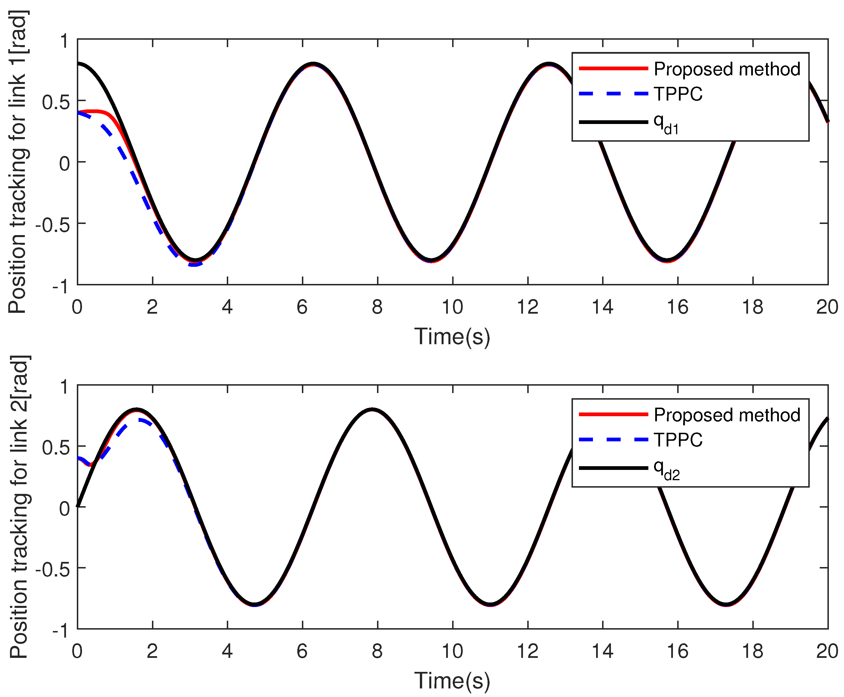
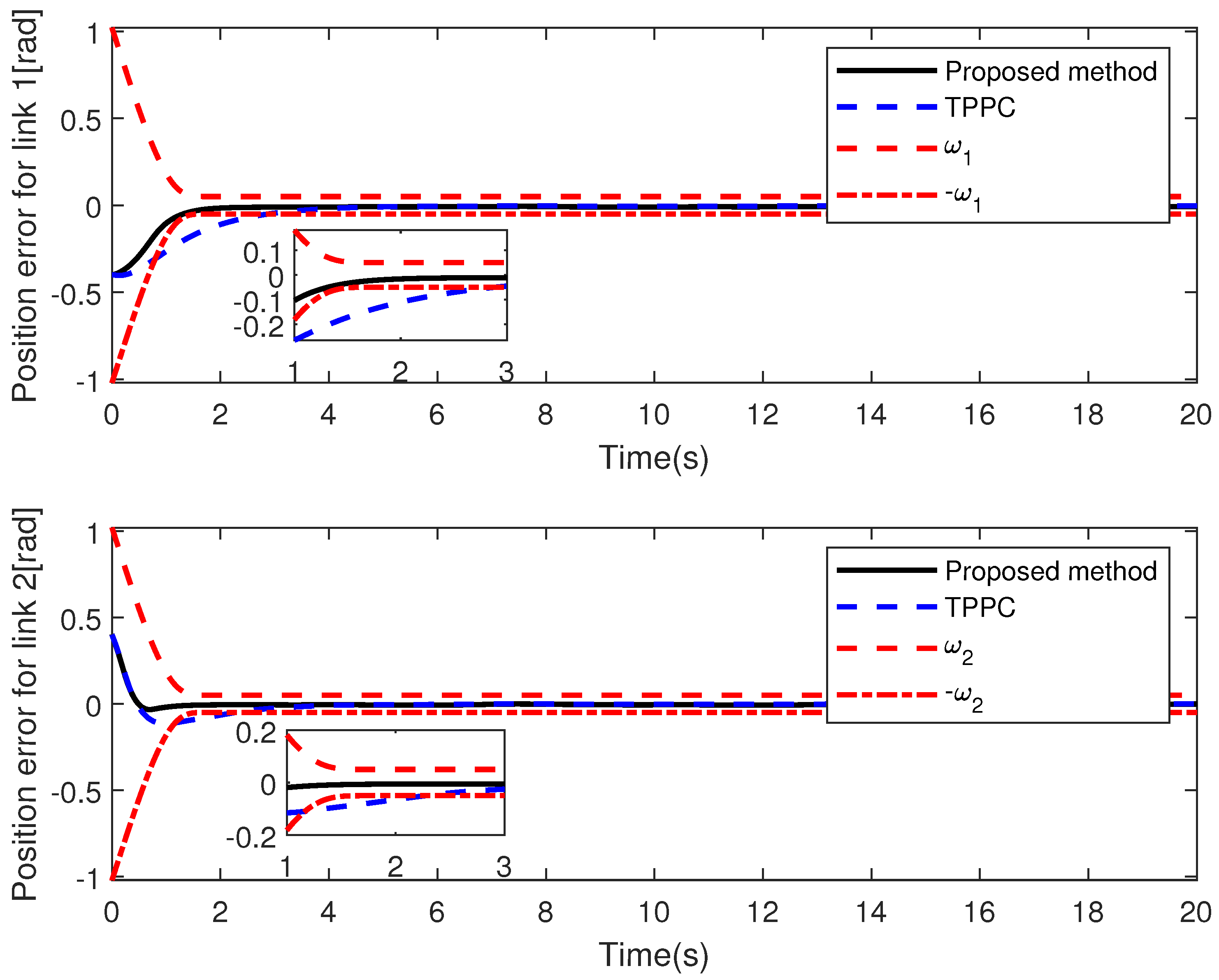
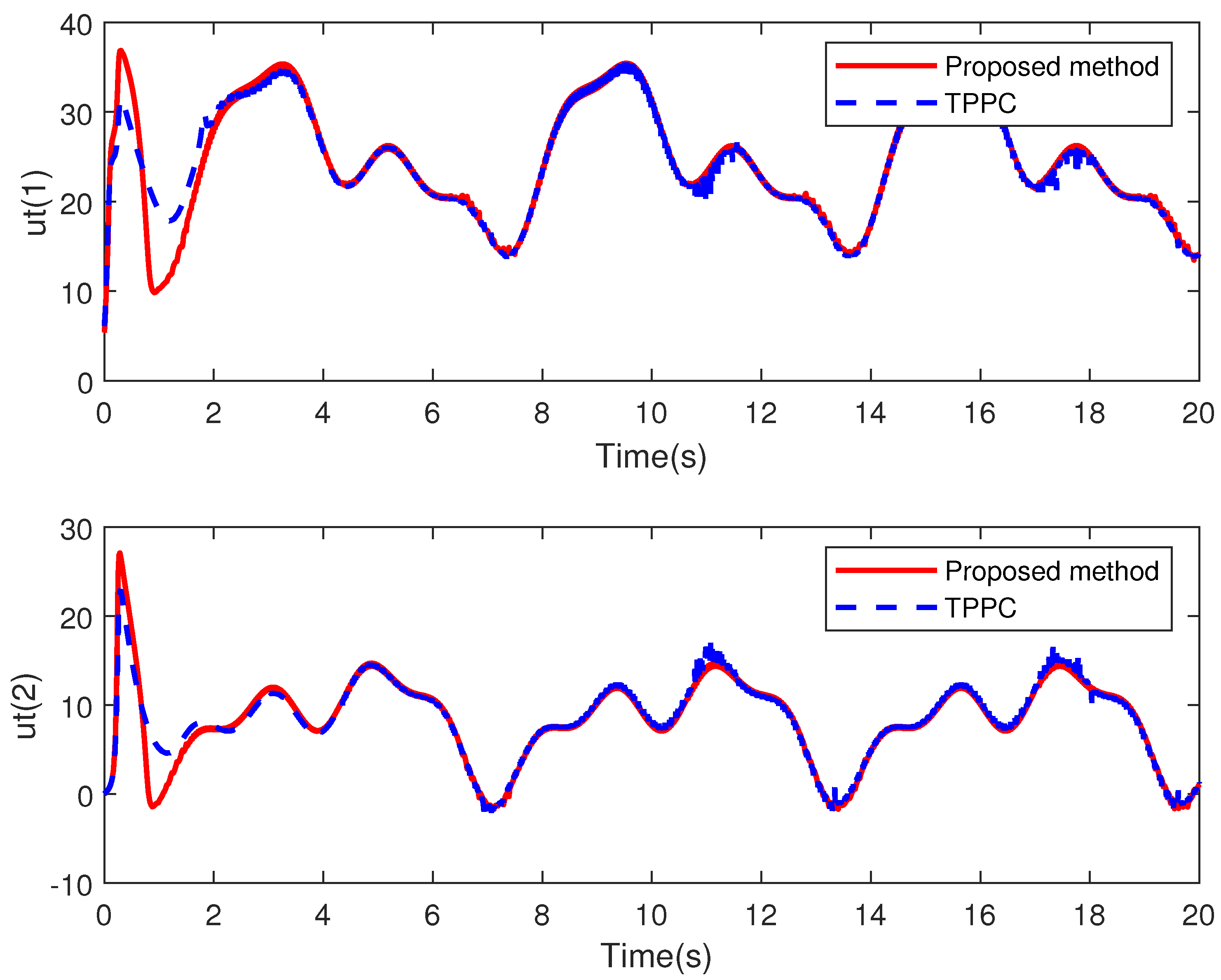
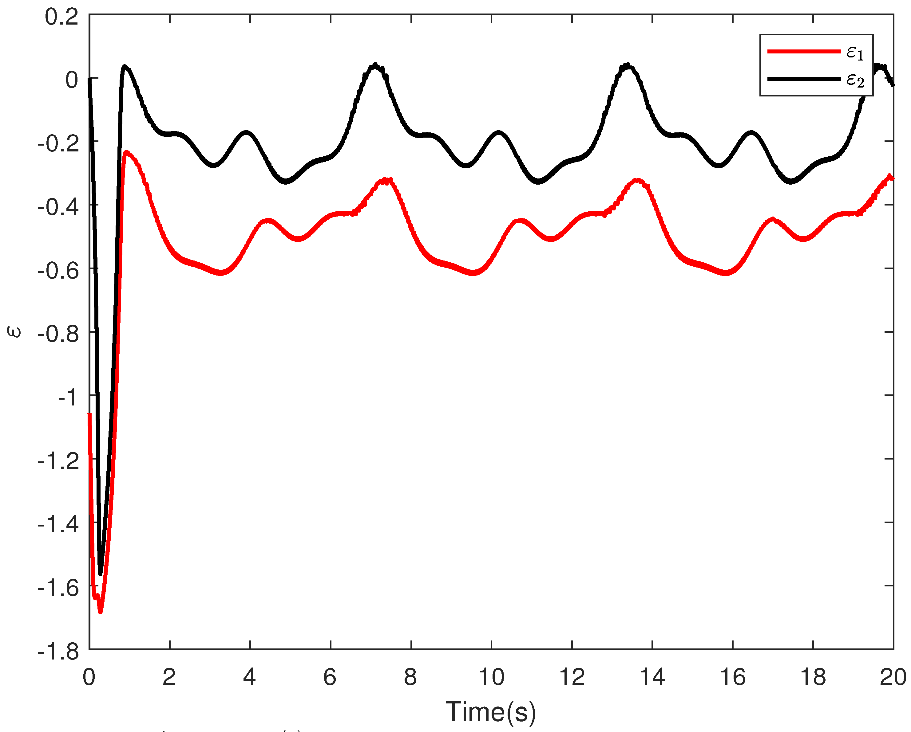
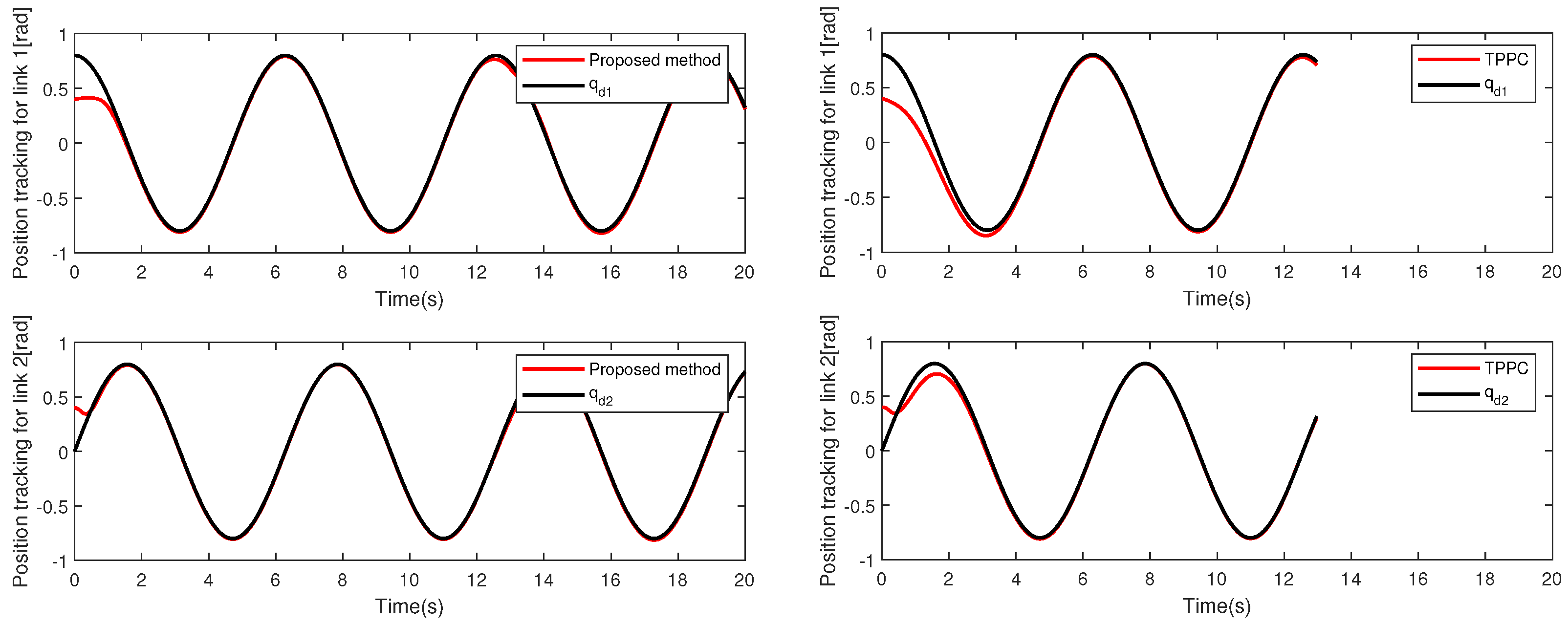
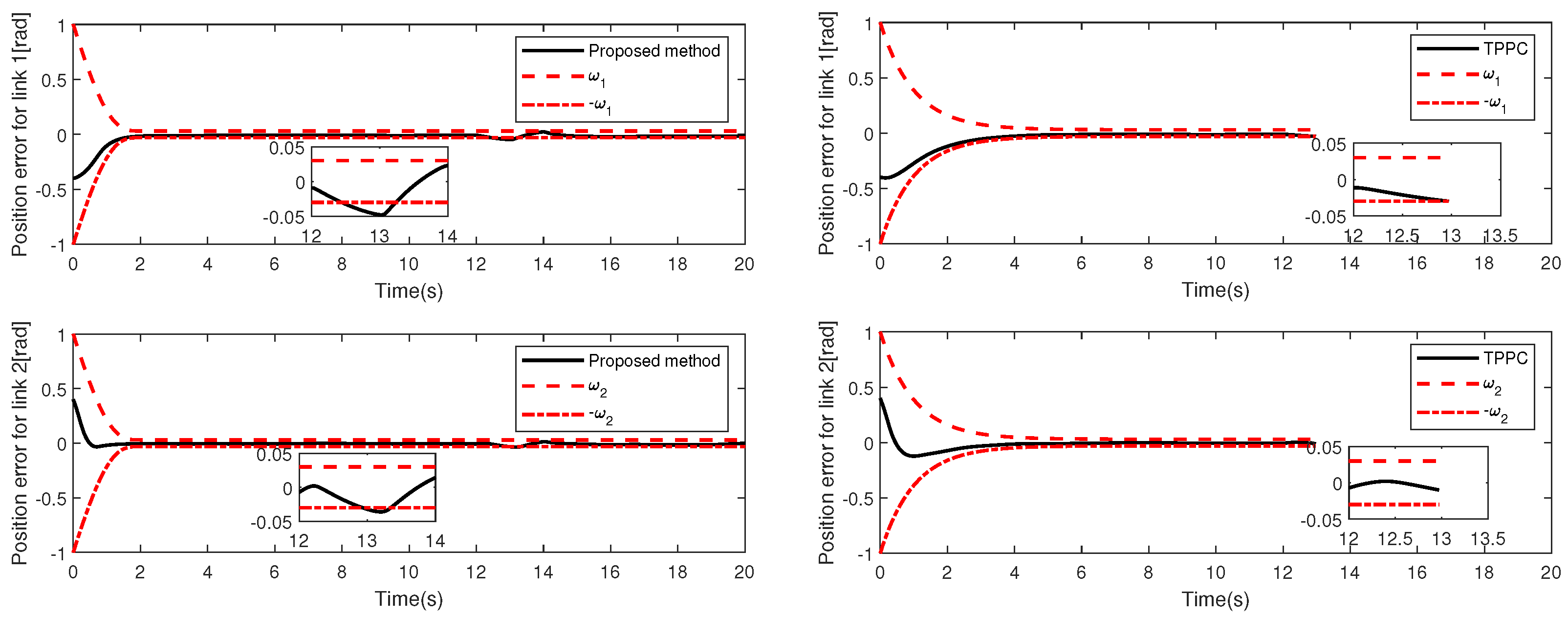
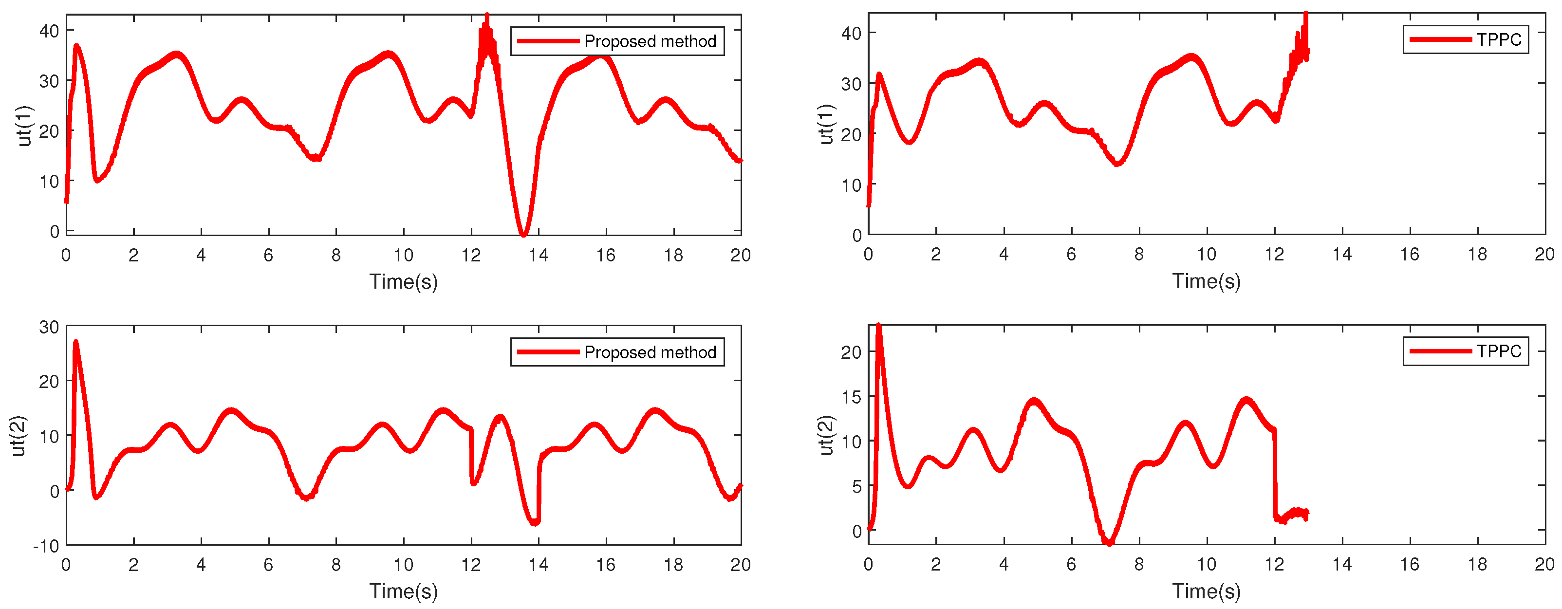
4. Simulation Verification

In this section, we have chosen the two-degrees-of-freedom manipulator model utilized in reference [33] as the simulation object for the purpose of validating the proposed controller Equation (28). The dynamics model is described as follows:

$$\begin{array}{cc}\hfill & M=\left[\begin{array}{cc}{m}_{11}& m_{12}\\ m_{21}& m_{22}\end{array}\right],C=\left[\begin{array}{cc}{c}_{11}& c_{12}\\ c_{21}& c_{22}\end{array}\right],G=\left[\begin{array}{c}{g}_1\\ g_2\end{array}\right],F=\left[\begin{array}{c}{f}_1\\ f_2\end{array}\right]\hfill \\ \hfill & m_{11}=(m_1+m_2)l_1^2+m_2{l}_2^2+2m_2{l}_1{l}_{2}cos\left(q_2\right)+J_1\hfill \\ \hfill & m_{12}=m_2{l}_2^2+m_2{l}_1{l}_{2}cos\left(q_2\right)\hfill \\ \hfill & m_{21}=m_2{l}_2^2+m_2{l}_1{l}_{2}cos\left(q_2\right)\hfill \\ \hfill & m_{22}=m_2{l}_2^2+J_2\hfill \\ \hfill & c_{11}=-m_2{l}_1{l}_{2}sin\left(q_2\right){\dot{q}}_2\hfill \\ \hfill & c_{12}=-m_2{l}_1{l}_{2}sin\left(q_2\right)({\dot{q}}_1+{\dot{q}}_2)\hfill \\ \hfill & c_{21}=m_2{l}_1{l}_{2}sin\left(q_2\right){\dot{q}}_1\hfill \\ \hfill & c_{22}=0\hfill \\ \hfill & g_1=(m_1+m_2)l_{1}gcos\left(q_2\right)+m_2{l}_{2}gcos(q_1+q_2)\hfill \\ \hfill & g_2=m_2{l}_{2}gcos(q_1+q_2)\hfill \\ \hfill & f_1=0.5sign\left({\dot{q}}_1\right)\hfill \\ \hfill & f_2=0.5sign\left({\dot{q}}_2\right)\hfill \end{array}$$

(44)

The parameters of the manipulator model align with the ones chosen in reference [33]: $m_1=0.5$ kg, $m_2=1.5$ kg, $l_1=1$ m, $l_2=0.8$ m, $J_1=5$ kg · m, $J_2=5$ kg · m, $g=9.8$ N/s². Due to the inherent uncertainty in parameter estimation during the modeling process, the nominal values of variables $m_1$ and $m_2$ have been chosen as $m_{10}=0.5$ kg and $m_{20}=1.5$ kg, respectively. Interference selection $d={[sin\left(4t\right)+0.5sin\left(200\pi t\right),cos\left(4t\right)+0.5sin\left(200\pi t\right)]}^{\mathrm{T}}$. The initial position and initial speed are selected as $q\left(0\right)={\left[\begin{array}{cc}0.4& 0.4\end{array}\right]}^{\mathrm{T}}$ and $\dot{q}\left(0\right)={\left[\begin{array}{cc}0& 0\end{array}\right]}^{\mathrm{T}}$, respectively. The expected trajectory is established as $q_d={\left[\begin{array}{cc}0.8cost& 0.8sint\end{array}\right]}^{\mathrm{T}}$. The selection of design parameters in the controller is as follows: $k_1=k_2=2$, ${\mathsf{\Lambda }}_1={\mathsf{\Lambda }}_2=20$, $T_s=2s$, ${\omega }_{0,1}={\omega }_{0,2}=1$, ${\omega }_{T_f,1}={\omega }_{T_f,2}=0.03$, $T_{\omega ,f1}=T_{\omega ,f2}=2s$, $\tau =0.2$.

Consider the following two cases:

Case 1: In this case, to effectively demonstrate the benefits of the proposed scheme, a comparison is made with the existing traditional PPC (TPPC) [32]. The simulation results are depicted in Figure 1, Figure 2, Figure 3 and Figure 4. Analysis of Figure 1, Figure 2 and Figure 3 demonstrates that the control strategy proposed in this study effectively guarantees that the tracking error remains within the prescribed range of the channel. From Figure 2, it can be obtained that compared with TPPC, the control method proposed in this paper has faster convergence speed, and can make the system tracking error maintain better performance, and the joint angle tracking effect is better. The control inputs of the two schemes are shown in Figure 3, and no high frequency chattering is shown. Figure 4 illustrates the boundedness of $\epsilon \left(t\right)$. When the controller structure is simplistic and the system model is entirely unknown, the proposed controller demonstrates commendable performance in trajectory tracking. Therefore, the controller in this paper achieves low complexity control and prescribed performance control.

Case 2: Furthermore, the following sudden disturbances are applied to verify the effectiveness of the proposed controller in addressing the fragility issues of the PPC. In order to better illustrate the unique advantages of the proposed scheme, the traditional PPC (TPPC) in reference [32] is employed as a comparison. Simulation results are displayed in Figure 5, Figure 6 and Figure 7. The tracking error is shown in Figure 6. Obviously, the existence of the shift function can effectively avoid the fragility issues commonly found in traditional PPC by shifting the error, even in the presence of unknown burst interference. In contrast, the system encounters significant error fluctuations and approaches the constraint boundary when subjected to sudden interference in TPPC. As a result, a control singularity arises around t = 12.8 s, leading to control failure. Therefore, the control strategy utilized in this paper effectively avoids the inherent fragility problem associated with the existing PPC and demonstrates better robustness in the presence of unknown disturbances.

$$\begin{array}{c}\hfill d=\left\{\begin{array}{cc}{\left[15sin\left(4t\right),-10cos\left(4t\right)\right]}^{\mathrm{T}},\hfill & 12s\le t\le 13s\hfill \\ 0,\hfill & else\hfill \end{array}\right.\end{array}$$

(45)

5. Conclusions

In this paper, a prescribed performance control method for robot systems with model uncertainties and unknown disturbances is proposed. This approach not only tackles the inherent fragility of the current prescribed performance control, but also substantially decreases the computational complexity of the controller. Aiming at the fragility issues of existing PPC, when the state of the controlled system experiences fluctuations caused by external interference, the constrained quantity is shifted by the shift function. Then, the influence of state fluctuations in the controlled system is mitigated, thereby preventing the occurrence of control singularities. Based on this, a novel prescribed performance controller without function approximator is developed. This approach significantly simplifies the design complexity of the controller. Finally, the efficacy of the proposed method and the existing PPC is substantiated through a comparative simulation analysis. Finally, the efficacy of this method in relation to the current PPC is confirmed through a comparative simulation analysis. Our next research direction is to extend the proposed approach to robotic systems with all-state constraints to achieve global performance.

References

1. Ferrara, A.; Incremona, G.P. Design of an integral suboptimal second-order sliding mode controller for the robust motion control of robot manipulators. IEEE Trans. Control. Syst. Technol. 2015, 23, 2316–2325. [Google Scholar] [CrossRef]
2. Jin, M.; Kang, S.H.; Chang, P.H.; Lee, J. Robust control of robot manipulators using inclusive and enhanced time delay control. IEEE/ASME Trans. Mechatron. 2017, 22, 2141–2152. [Google Scholar] [CrossRef]
3. Incremona, G.P.; Ferrara, A.; Magni, L. MPC for robot manipulators with integral sliding modes generation. IEEE/ASME Trans. Mechatron. 2017, 22, 1299–1307. [Google Scholar] [CrossRef]
4. Yang, P.; Su, Y. Proximate fixed-time prescribed performance tracking control of uncertain robot manipulators. IEEE/ASME Trans. Mechatron. 2021, 27, 3275–3285. [Google Scholar] [CrossRef]
5. Yang, P.; Su, Y.; Zhang, L. Proximate fixed-time fault-tolerant tracking control for robot manipulators with prescribed performance. Automatica 2023, 157, 111262. [Google Scholar] [CrossRef]
6. Huang, H.; He, W.; Li, J.; Xu, B.; Yang, C.; Zhang, W. Disturbance observer-based fault-tolerant control for robotic systems with guaranteed prescribed performance. IEEE Trans. Cybern. 2020, 52, 772–783. [Google Scholar] [CrossRef] [PubMed]
7. Vo, A.T.; Truong, T.N.; Kang, H.J. Fixed-Time RBFNN-Based Prescribed Performance Control for Robot Manipulators: Achieving Global Convergence and Control Performance Improvement. Mathematics 2023, 11, 2307. [Google Scholar] [CrossRef]
8. Li, Z.; Wang, Y.; Song, Y.; Ao, W. Global consensus tracking control for high-order nonlinear multiagent systems with prescribed performance. IEEE Trans. Cybern. 2022, 53, 6529–6537. [Google Scholar] [CrossRef] [PubMed]
9. Hu, H.; Chen, S.; Zhao, J.; Luo, J.; Jia, S.; Zhou, J.; Zhang, J.; Xiong, C.; Zhang, C.; Yang, G. Robust adaptive control of a bimanual 3T1R parallel robot with gray-box-model and prescribed performance function. IEEE/ASME Trans. Mechatron. 2022, 29, 466–475. [Google Scholar] [CrossRef]
10. Khoshnam, S.; Ali, K.; Abbas, C. An observer-based neural adaptive PID2 controller for robot manipulators including motor dynamics with a prescribed performance. IEEE/ASME Trans. Mechatron. 2020, 26, 1689–1699. [Google Scholar]
11. Khoshnam, S. Coordinated saturated output-feedback control of an autonomous tractor-trailer and a combine harvester in crop-harvesting operation. IEEE Trans. Veh. Technol. 2021, 71, 1224–1236. [Google Scholar]
12. Huang, J.; Ri, S.; Fukuda, T.; Wang, Y. A disturbance observer based sliding mode control for a class of underactuated robotic system with mismatched uncertainties. IEEE Trans. Autom. Control. 2018, 64, 2480–2487. [Google Scholar] [CrossRef]
13. Yang, Y.; Xu, H.; Yao, X. Inverse-Dynamics-and disturbance-Observer-Based tube model predictive tracking control of uncertain robotic manipulator. J. Frankl. Inst. 2023, 360, 6906–6927. [Google Scholar] [CrossRef]
14. Chen, X.; Zhao, F.; Liu, Y.; Liu, H.; Huang, T.; Qiu, J. Reduced-order observer-based preassigned finite-time control of nonlinear systems and its applications. IEEE Trans. Syst. Man Cybern. Syst. 2023, 53, 4205–4215. [Google Scholar] [CrossRef]
15. Guo, Z.; Ma, Q.; Guo, J.; Zhao, B.; Zhou, J. Performance-Involved Coupling Effect-Triggered Scheme for Robust Attitude Control of HRV. IEEE/ASME Trans. Mechatron. 2020, 25, 1288–1298. [Google Scholar] [CrossRef]
16. Hu, Y.; Yan, H.; Zhang, Y.; Zhang, H.; Chang, Y. Event-Triggered Prescribed Performance Fuzzy Fault-Tolerant Control for Unknown Euler-Lagrange Systems With Any Bounded Initial Values. IEEE Trans. Fuzzy Syst. 2023, 31, 2065–2075. [Google Scholar] [CrossRef]
17. Bu, X.; Lv, M.; Lei, H.; Cao, J. Fuzzy Neural Pseudo Control With Prescribed Performance for Waverider Vehicles: A Fragility-avoidance Approach. IEEE Trans. Cybern. 2023, 53, 4986–4999. [Google Scholar] [CrossRef] [PubMed]
18. Bu, X.; Lei, H. A fuzzy wavelet neural network-based approach to hypersonic flight vehicle direct nonaffine hybrid control. Nonlinear Dyn. 2018, 94, 1657–1668. [Google Scholar] [CrossRef]
19. Bu, X.; Qi, Q.; Jiang, B. A simplified finite-time fuzzy neural controller with prescribed performance applied to waverider aircraft. IEEE Trans. Fuzzy Syst. 2021, 30, 2529–2537. [Google Scholar] [CrossRef]
20. Song, Y.; Tuo, Y.; Li, J. A neural adaptive prescribed performance controller for the chaotic PMSM stochastic system. Nonlinear Dyn. 2023, 111, 15055–15073. [Google Scholar] [CrossRef]
21. Liu, Y.; Liu, X.; Jing, Y. Adaptive fuzzy finite-time stability of uncertain nonlinear systems based on prescribed performance. Fuzzy Sets Syst. 2019, 374, 23–39. [Google Scholar] [CrossRef]
22. Bu, X.; Jiang, B.; Lei, H. Nonfragile quantitative prescribed performance control of waverider vehicles with actuator saturation. IEEE Trans. Aerosp. Electron. Syst. 2022, 58, 3538–3548. [Google Scholar] [CrossRef]
23. Bu, X.; Jiang, B.; Lei, H. Low-complexity fuzzy neural control of constrained waverider vehicles via fragility-free prescribed performance approach. IEEE Trans. Fuzzy Syst. 2023, 31, 2127–2139. [Google Scholar] [CrossRef]
24. Zhou, H.; Sui, S.; Tong, S. Finite-Time Adaptive Fuzzy Prescribed Performance Formation Control for High-Order Nonlinear Multiagent Systems Based on Event-Triggered Mechanism. IEEE Trans. Fuzzy Syst. 2022, 31, 1229–1239. [Google Scholar] [CrossRef]
25. Gao, Z.; Zhang, Y.; Guo, G. Finite-time fault-tolerant prescribed performance control of connected vehicles with actuator saturation. IEEE Trans. Veh. Technol. 2022, 72, 1438–1448. [Google Scholar] [CrossRef]
26. Deng, W.; Zhou, H.; Zhou, J.; Yao, J. Neural network-based adaptive asymptotic prescribed performance tracking control of hydraulic manipulators. IEEE Trans. Syst. Man Cybern. Syst. 2022, 53, 285–295. [Google Scholar] [CrossRef]
27. He, W.; Huang, H.; Ge, S.S. Adaptive neural network control of a robotic manipulator with time-varying output constraints. IEEE Trans. Cybern. 2017, 47, 3136–3147. [Google Scholar] [CrossRef] [PubMed]
28. Zhang, J.X.; Yang, G.H. Fault-tolerant output-constrained control of unknown Euler–Lagrange systems with prescribed tracking accuracy. Automatica 2020, 111, 108606. [Google Scholar] [CrossRef]
29. Zhang, L.; Su, Y.; Wang, Z. A simple non-singular terminal sliding mode control for uncertain robot manipulators. Proc. Inst. Mech. Eng. Part I J. Syst. Control. Eng. 2019, 233, 666–676. [Google Scholar] [CrossRef]
30. Liang, J.; Chen, Y.; Lai, N.; He, B.; Miao, Z.; Wang, Y. Low-complexity prescribed performance control for unmanned aerial manipulator robot system under model uncertainty and unknown disturbances. IEEE Trans. Ind. Inform. 2022, 18, 4632–4641. [Google Scholar] [CrossRef]
31. Lu, M.; Liu, L.; Feng, G. Adaptive tracking control of uncertain Euler–Lagrange systems subject to external disturbances. Automatica 2019, 104, 207–219. [Google Scholar] [CrossRef]
32. Bechlioulis, C.P.; Rovithakis, G.A. A low-complexity global approximation-free control scheme with prescribed performance for unknown pure feedback systems. Automatica 2014, 50, 1217–1226. [Google Scholar] [CrossRef]
33. Su, Y.; Zheng, C.; Mercorelli, P. Robust approximate fixed-time tracking control for uncertain robot manipulators. Mech. Syst. Signal Process. 2020, 135, 106379. [Google Scholar] [CrossRef]
Figure 1. Tracking performance in case 1.
Electronics 13 01417 g001
Figure 2. Tracking errors and the prescribed bounds in case 1.
Electronics 13 01417 g002
Figure 3. Control input in case 1.
Electronics 13 01417 g003
Figure 4. Transform error ε ( t ) in case 1.
Electronics 13 01417 g004
Figure 5. Position tracking error in case 2.
Electronics 13 01417 g005
Figure 6. Position tracking error in case 2.
Electronics 13 01417 g006
Figure 7. Control input in case 2.
Electronics 13 01417 g007
Disclaimer/Publisher’s Note: The statements, opinions and data contained in all publications are solely those of the individual author(s) and contributor(s) and not of MDPI and/or the editor(s). MDPI and/or the editor(s) disclaim responsibility for any injury to people or property resulting from any ideas, methods, instructions or products referred to in the content.