1. Introduction
As the core component of the Fourier-transform infrared spectrometer (FTIR), the Michelson interferometer generates an optical path difference by means of a moving mirror [
1]. Therefore, the control accuracy of the moving mirror control system determines the performance of the FTIR [
2]. Today, swing-arm interferometers have the advantage of high stability and are widely used in FTIR [
3]. Moving mirrors of swing-arm interferometers are mostly driven by rotary voice coil motors (RVCMs). RVCMs are special motors that only work in a limited angle range, and they are commonly used for reciprocating drives with small inertial load [
4]. Compared with traditional motors, RVCMs have the exceptional advantages of small dimensions, high accuracy, large thrust, and fast response [
5]. Therefore, RVCMs are widely used in the industrial, aerospace, and precision instrument fields [
6,
7,
8,
9].
However, in RVCM-based control systems, external disturbances act directly on the motor. External random disturbances (such as vibration disturbances) are not considered in the mechanical balance equation of the model, and parameter perturbations are not considered in the electrical balance equation. These disturbances and parameters change as the system runs for a long time and is affected by factors such as temperature, device aging, and working environment [
10]. These uncertainties lead to poor robustness and weak anti-interference ability of the control system. In recent years, with the rapid development of control theory, some advanced control methods have been proposed to improve the performance of VCM-based control systems, such as the control method with a disturbance observer [
11], a position estimator [
12], adaptive control [
13,
14], sliding mode control [
15,
16,
17], active disturbance rejection control (ADRC) [
18], and other advanced control technologies.
ADRC is a nonlinear control method that does not depend on the precise mathematical model of the controlled object. It can estimate the total disturbance of the system in real time and then compensate the system to improve its anti-interference ability [
19]. At present, ADRC is widely used in the field of motor control. In [
20], it is verified that ADRC can effectively observe the bounded time-varying disturbance of voice coil motor control systems. In [
21], linear ADRC is used to reduce the calculation load of the controller and is suitable for real-time control systems. In [
22], improved ADRC applied to high-precision positioning workbench is proposed, which effectively improves the positioning accuracy and robustness of the system. The majority of the above ADRC studies focus on the controller’s structure rather than how to adjust its parameters, which limits the promotion and application of ADRC to a certain extent.
Conventional ADRC has many parameters, and each parameter directly and significantly affects the controller’s performance. To fully exploit the advantages of ADRC, its parameters must be properly adjusted. The manual adjustment of ADRC parameters requires the expertise of engineers, which is time-consuming and labor-intensive, so it is difficult to achieve ideal control. Second, the range of ADRC parameters varies as a result of the various controlled objects. Manual adjustment is not conducive to the widespread application of ADRC. Therefore, it is necessary to find a parameter tuning method that is convenient for application.
To address this issue, numerous scholars have proposed the use of heuristic algorithms to tune the parameters of ADRC. In [
23], genetic algorithm (GA)-based parameter tuning ADRC was proposed to improve the stabilization accuracy of the three-axis inertial platform. However, since the GA is prone to premature convergence and has poor local search capabilities, it can only find suboptimal solutions, as opposed to the optimal one. Particle swarm optimization (PSO) is also a commonly used parameter optimization algorithm. However, the search ability of PSO is weaker in the later stage of the iterations, and it can easily fall into local optima. In [
24], an improved PSO was proposed to balance the global and local search abilities of PSO. Reference [
25] proposed using the butterfly optimization algorithm to tune the parameters of ADRC to achieve the best performance of the controller. In [
26], ant colony optimization (ACO) was applied to the control of current controllers. However, setting ACO parameters is complex, and it is easy to deviate from the high-quality solution if the parameters are not set properly. Compared with ACO, gray wolf optimization (GWO) has the advantages of a simple structure and fewer parameters [
27]. However, GWO has the drawbacks of low accuracy and slow convergence when facing complex problems. The chimp optimization algorithm suffers from the same shortcomings [
28]. In [
29], a whale optimization algorithm (WOA) was applied to fine-tune the parameters of ADRC. However, the WOA easily falls into local optima, and its optimization ability is weak. The sparrow search algorithm (SSA) has also been used in ADRC parameter tuning [
30,
31]. It has strong local search ability and fast convergence, but its global search ability is weak and it does not easily escape the local optimum. In addition, some hybrid algorithms have also been proposed, like the algorithm composed of differential evolution and PSO [
32] and that composed of PSO and bacterial foraging optimization (BFO) [
33].
The snake optimization (SO) algorithm is a heuristic algorithm that simulates the feeding and breeding behavior of snakes [
34]. This algorithm has the advantages of a strong global search ability, high efficiency, and fast convergence. As a reference, the SO algorithm was tested using 10 functions at the Congress on Evolutionary Computation (CEC) 2020. The SO algorithm performed poorly on tests of four functions due to its weak local search capabilities in the later stages of the search. To address this issue, this study designed an improved SO algorithm (I-SO). It adopts the chaotic elite opposition learning algorithm and introduces the sine and cosine (SC) search mode, which enhances the global search capability of SO and its ability to escape local optima.
In this paper, to improve the control of ADRC for a moving mirror control system and eliminate the time-consuming and labor-intensive process of manual parameter adjustment, a novel ADRC system with parameter autotuning based on I-SO is proposed. ADRC with parameter autotuning based on I-SO is more robust than conventional ADRC. As a population-based optimization algorithm, I-SO does not rely on specific mathematical models, thus enhancing the applicability of ADRC with parameter autotuning based on I-SO in the control field. The simulation results show the feasibility and the effectiveness of the proposed method.
The rest of this paper is organized as follows.
Section 2 describes the structure of the moving mirror system and the mathematical model of an RVCM. The principle of ADRC is also explained in this section.
Section 3 provides a brief overview of the original SO and describes the proposed I-SO in detail. Further,
Section 3 describes the implementation process of I-SO applied in ADRC.
Section 4 demonstrates the superiority of I-SO and verifies the advantages of I-SO by comparison with various optimization algorithms.
Section 5 simulates a moving mirror control system and verifies the effectiveness of the ADRC with parameter autotuning based on I-SO.
Section 6 presents the conclusions of this research.
3. ADRC with Parameter Autotuning Based on the I-SO Algorithm
3.1. Basic Principles of SO
The SO algorithm is inspired by the mating behavior of snakes. If the temperature is low and food is available, snakes will try to find the best mate and then mate. Otherwise, they will only look for food or eat existing food. Each snake has a position in the search space, which is modified by looking for food, fighting, and mating to find the globally optimal position. Therefore, the mechanism of SO consists of the exploration phase without food and the exploitation phase of existing food, explained as follows.
Before exploring, the temperature of the environment, the food quantity in the environment, and the population of snakes are first defined.
The temperature
is defined as:
where
is the current number of iterations and
is the maximum number of iterations.
The food quantity
is defined as:
where
is a constant.
For the snake population, the initialization of snakes is performed by generating a uniformly distributed random population, as shown in Equation (11):
where
is the position of the
i-th individual,
and
are, respectively, the lower and upper bounds of the environment, and
is a random number between 0 and 1.
Assuming that the number of females and males in the population of snakes is the same, then:
where
is the number of males,
the number of females, and
the total number of individuals in the snake population.
3.1.1. Exploration Phase without Food
If
< threshold (threshold of food quantity), the snakes look for food by selecting any random position and update their position accordingly. The position update equations of male and female snakes are shown in Equation (13):
where
is the
i-th male snake position,
is the
i-th female snake position,
and
refer to the positions of random male and female, respectively,
is a constant, and
is the male ability to find food. Correspondingly,
is the female ability to find food. These can be calculated using Equation (14):
where
is the fitness of
and
is the fitness of the
i-th individual in the male group, and the same can be seen for the female group in Equation (14).
3.1.2. Exploitation Phase of Existing Food
Under the condition of
>= threshold, if
> threshold (temperature threshold), the environment is in a hot state. The snakes only look for food, and the position update equation is shown in Equation (15):
where
is the position of an individual,
is the position of the best individual, and
is a constant.
If
< threshold (temperature threshold), the temperature is cold. The snakes will either be in fight mode or in mating mode. The fight mode can be described by Equation (16):
where
is the
i-th male position,
refers to the position of the best individual in the female group,
is a constant, and
is the fighting ability of the male snake. Similarly,
and
can be understood.
and
can be obtained from Equation (17):
where
is the fitness of the best snake of the female group,
is the fitness of the best snake of the male group, and
is the fitness of the
i-th snake position.
The mating mode can be described by Equation (18):
where
is the
i-th male position and
is the
i-th female position in their respective groups.
and
refer to the mating ability of the males and females, respectively, and they can be calculated as follows:
where
is the fitness of the
i-th female of the female group and
is the fitness of the
i-th male of the male group.
When two snakes complete mating, their egg may or may not hatch. If the egg hatches, the worst male and female are replaced, as described in Equation (20):
where
is the worst male individual and
is the worst female.
3.2. I-SO
3.2.1. Chaotic Elite Opposition Learning
To enhance the global search ability of the SO algorithm, we aimed at improving the quality of its initial solution. In this paper, the chaotic elite opposition learning algorithm is applied to the initialization phase of SO. The chaotic values generated by the tent chaotic map are uniformly distributed in the range of 0–1 [
38]. Elite opposition learning exploits elite individuals having more effective information to construct their opposition population and selects multiple excellent individuals from the current population and the opposition population as the initial solution, thus improving the quality of the initial population [
39]. The definition of a tent chaotic map is shown in Equation (21):
where
is a random number within the range of 0–1.
The distribution and frequency of chaotic values of the tent chaotic map are shown in
Figure 3a,b, where it can be seen that the chaotic values generated by the tent chaotic map are uniformly distributed between 0 and 1 and show rich diversity.
Suppose that
is an elite individual in the search space. The definition of its reverse solution
is shown in Equation (22):
where
and
are the lower and upper boundaries of the
dimension search space, respectively, and
is a random number between 0 and 1.
The steps to initialize the population using the chaotic elite opposition learning algorithm are as follows.
(1) Use the tent chaotic map to initialize population S, calculate the fitness of individual, and select the first N/2 individuals with better fitness to form elite population E.
(2) Calculate the opposition population OE of elite population E.
(3) The new population {S, OE} is obtained by merging populations S and OE, and the fitness of individuals in the new population is calculated. The final initial population is composed of the first N{S, OE}/2 individuals with better fitness.
This paper combines a tent chaotic map with the elite opposition learning algorithm to maintain the diversity of the population and improve the quality of the initial population.
3.2.2. SC Search Mode
In the exploration phase of existing food, in order to enhance the ability of the SO algorithm to escape the local optimum, the algorithm introduces a SC search mode [
40], which requires the algorithm to use a mathematical model based on sine and cosine functions to fluctuate outward. We modify Equation (15), (16), and (18), and the modified part is shown in Equation (23).
The position update formula for males introduces the sine function, and for females, the cosine function is introduced.
The chaotic elite opposition learning algorithm improves the quality of the initial solution, and the introduction of the SC search mode enhances the ability of SO to escape the local optimum. These two strategies are helpful for the SO to find the global optimum solution.
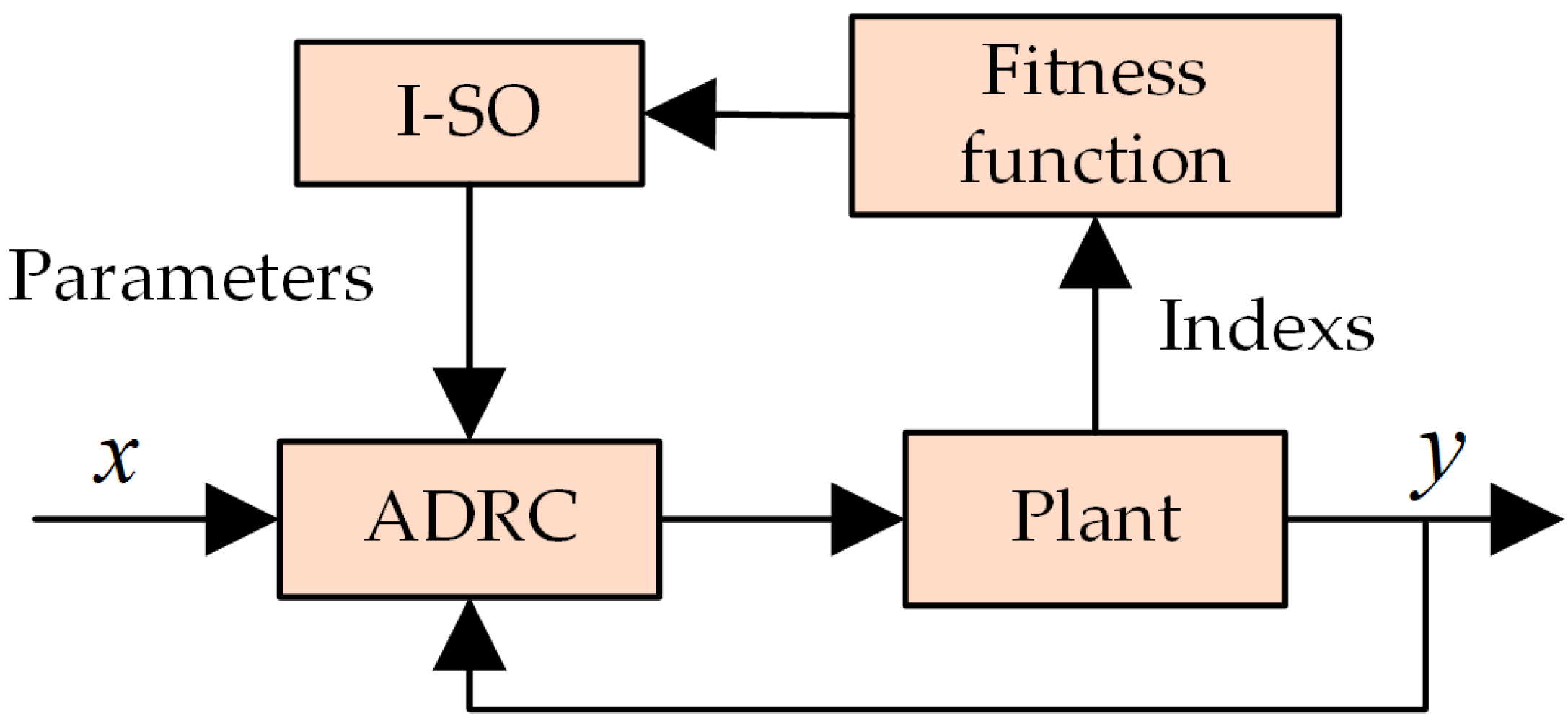
3.3. Implementation of I-SO Applied in ADRC
In this paper, I-SO is implemented to optimize the parameters of ADRC in the control system of an RVCM. The schematic diagram of the control system including I-SO is shown in
Figure 4. In detail, the tunable and key parameters
,
,
, and
are optimized via I-SO under the consideration of the stability and accuracy of the system. The fitness function determines the changing trend of the snake’s position. Therefore, an appropriate fitness function to connect I-SO and ADRC is needed to obtain appropriate parameters for ADRC.
Generally, the control indicators of the RVCM and other control systems include stable and dynamic performance indicators. When the input of the system is a step response, the important dynamic performance indicators of the system include overshoot and rise time . The steady-state performance indicator is mainly stable error . A system with excellent performance needs to consider stable and dynamic performance.
Integrated time and absolute error (ITAE) is an indicator used to measure system performance. In this paper, the
is used to measure the LESO’s observation error of total disturbance to the system. The expression of
is:
where
is the response period of the system and
is the observation error of the total disturbance to the system. The expression of
is:
Finally, the fitness function
is composed of the weighted sum of the dynamic and stable control indicators and
, as shown in Equation (26):
where
,
,
, and
are the weights.
The dynamic and stable control indicators and share the same characteristic that the smaller their value is, the better the control of the RVCM that will be achieved. Thus, the ideal parameters can cause the system to have the best control and enable the fitness function to reach the minimum. In each iteration, the optimization process of I-SO is the process of moving the position of each snake towards the optimal position.
In the experiment, the detailed optimization process of I-SO computing the optimization parameters , , , and can be described as follows.
Step 1. The parameters in I-SO are initialized, including the number of snakes , the maximum number of iterations , the dimension , the upper limit and the lower limit of the search space, and thresholds of food quantity and temperature, etc. The position of each snake in the search space is initialized via the chaotic elite opposition learning algorithm.
Step 2. The snake population is divided into two groups, one for males and the other for females.
Step 3. ADRC is run with the parameters of Step 1, and the RVCM is controlled by the ADRC. The indicators of control of the system are calculated. These indicators are substituted into Equation (26) to calculate the value of the fitness function. The results are compared and the best males and females are defined.
Step 4. The iteration is executed and the food quantity and temperature are calculated according to Equations (9) and (10).
Step 5. The stage of exploring food is entered and the positions of males and females are updated according to Equation (13).
Step 6. When the amount of food is sufficient, the next stage is entered to judge whether the temperature is appropriate. The position of the snake is updated using Equations (15), (16) and (18), which introduce the SC search mode.
Step 7. The stopping criterion is checked. If the number of iterations is greater than the maximum number of iterations , the optimal parameters are output and the algorithm is stopped. Otherwise, the process moves to Step 4.
The pseudocode of Algorithm 1 I-SO is as follows.
| Algorithm 1 I-SO |
| 1: | Initialize parameters of I-SO |
| 2: | Initialize the snakes using Equation (22) |
| 3: | Equally divide the population into two groups |
| 4: | ) |
| 5: | Evaluate the fitness of individuals in each group |
| 6: | Find best male
and best female
|
| 7: | Define Temp using Equation (9). |
| 8: | Define food Quantity Q using Equation (10). |
| 9: | if (Q < 0.25) then |
| 10: | Perform exploration using Equation (13). |
| 11: | else |
| 12: | if (temp> 0.6) then |
| 13: | Perform exploitation Equations (15) and (23) |
| 14: | else |
| 15: | if (rand > 0.6) then |
| 16: | Snakes in Fight Mode Equations (16) and (23) |
| 17: | else |
| 18: | Snakes in Mating Mode Equations (18) and (23) |
| 19: | Change the worst male and female using Equation (20) |
| 20: | end if |
| 21: | end if |
| 22: | end if |
| 23: | end while |
| 24: | Return best solution. |
4. Simulation Results and Analysis
To verify the effectiveness of the I-SO, an ADRC model of the RVCM was established using MATLAB, and the key parameters of ADRC were tuned through I-SO. The environment configuration of this simulation experiment was as follows: a 64-bit Windows 10 operating system, an Intel (R) Core (TM) i7-10710u CPU, a main frequency of 1.10 GHz, 16 GB of memory, and simulation software MATLAB R2016b.
According to the commissioning experience, the general parameters of the control system were set as follows:
TD: , ; LESO: ; SEF:
In order to test the observation ability of the LESO for the total disturbance of system, a disturbance was introduced into the speed link of the system. The anti-interference ability of the system can be verified by adding different disturbances and noises in different links of the system. When conducting vibration tests on instruments or models in the field or in the laboratory, sinusoidal vibration tests are often used. Introducing sinusoidal periodic disturbances can simulate disturbances in the environment by adjusting the frequency, vibration amplitude, and test duration. Therefore, the expression for the disturbance was set to:
- (2)
SO algorithm: the parameter settings of I-SO algorithm are shown in
Table 1.
The minimum value of the fitness function, the convergence speed, and the standard deviation (STD) of multiple different minimum fitness function values obtained after repeatedly running the algorithm need to be considered important indicators of the intelligent optimization algorithm. The minimum value of the fitness function reflects the search ability of the algorithm, and the standard deviation reflects its stability.
The optimization algorithm was run 50 times independently, and the average of 50 convergence speed values was calculated, as well as the average and standard deviation of 50 fitness function values. Among the 50 running results, the operation result of the algorithm whose convergence speed and fitness function value were closest to their respective averages (the average value of the fitness function was first considered) was selected as the operation result of optimization algorithm (each optimization algorithm mentioned below was handled in this same way).
4.1. Verification of Control Performance of ADRC Tuned by I-SO
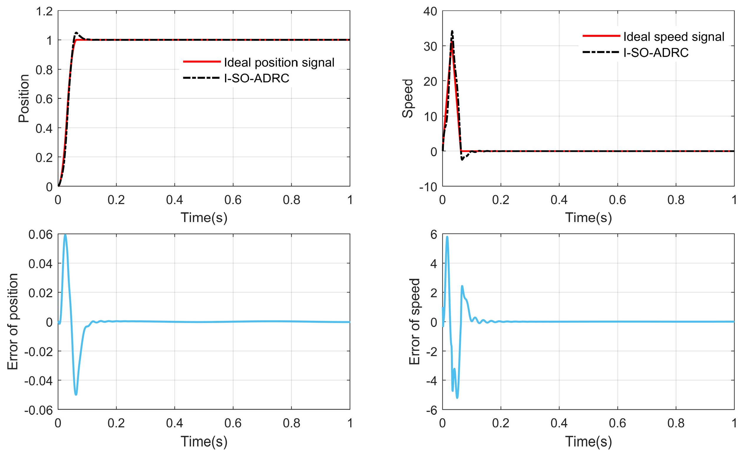
After selection, we finally determined that the optimal solution output by I-SO algorithm is {178, 49,642, 7,898,000, 145}.
Figure 5 shows the response curves and error curves.
Table 2 shows fitness function values and some control indicators. It can be seen from
Figure 5 and
Table 2 that the parameters calculated by I-SO can enable the simulation system to achieve outstanding dynamic and stable performance, as well as an exceptional response to position and speed signals. When there is no disturbance in the system, the position overshoot is 4.66%, both the position and speed steady-state error are 0, and the rise time is shorter than 0.1 s. When there is disturbance in the system, the system has a small steady-state error of about 0.02%.
Figure 6 shows the observation results provided by the LESO with disturbance in the system. It can be seen from
Figure 6 that the observation results of the position signal and speed signal are satisfactory. It can be seen from
Figure 6 that the LESO cannot effectively observe the disturbance at the initial stage due to the large initial error when the system tracks the step signal, but after about 0.1 s, the LESO can effectively observe the disturbance introduced by the system.
4.2. Convergence Verification of I-SO–ADRC
As a control algorithm combined with an intelligent optimization algorithm, it is necessary to verify the convergence of I-SO and ADRC.
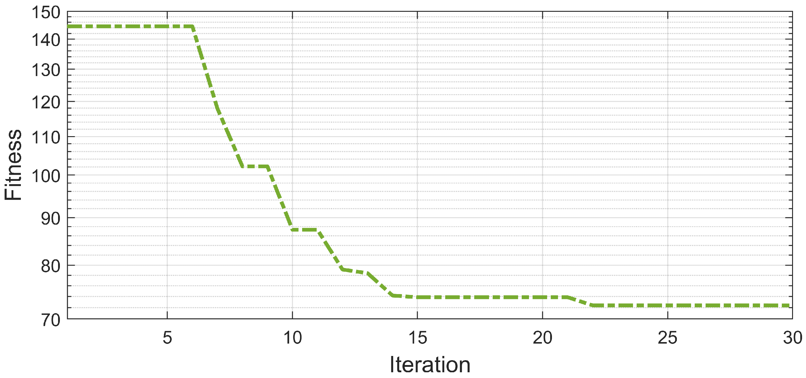
Figure 7 shows the convergence curve of the fitness function in the I-SO optimization process. It can be seen from
Figure 7 that the value of the fitness function gradually decreases with the increase in the number of iterations and does not change after iteration 22, indicating that I-SO is convergent.
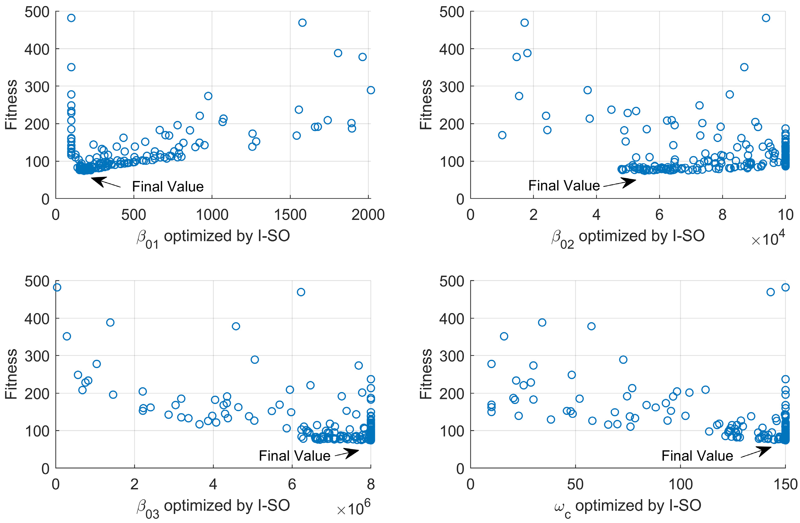
Figure 8 depicts the optimization process of each parameter by I-SO in the form of a scatter diagram, which is complex. By observing the distribution of scatter points, it can be seen that the value of each parameter changes with the value of the fitness function, and finally converges to the optimal parameter value.
In
Figure 7, it can be seen that the fitness is greatly reduced at iterations 6, 9, and 22, which is representative of the iterative process. The parameter sets obtained for iterations 6, 9, and 22 are {950, 99,317, 7,442,311, 75}, {217, 50,420, 7,277,566, 80}, and {178, 49,642, 7,898,000, 145}, respectively. In order to verify the I-SO–ADRC convergence and the applicability of I-SO to tune the parameters of ADRC, the optimization results of iterations 6, 9, and 22 are compared in
Figure 9.
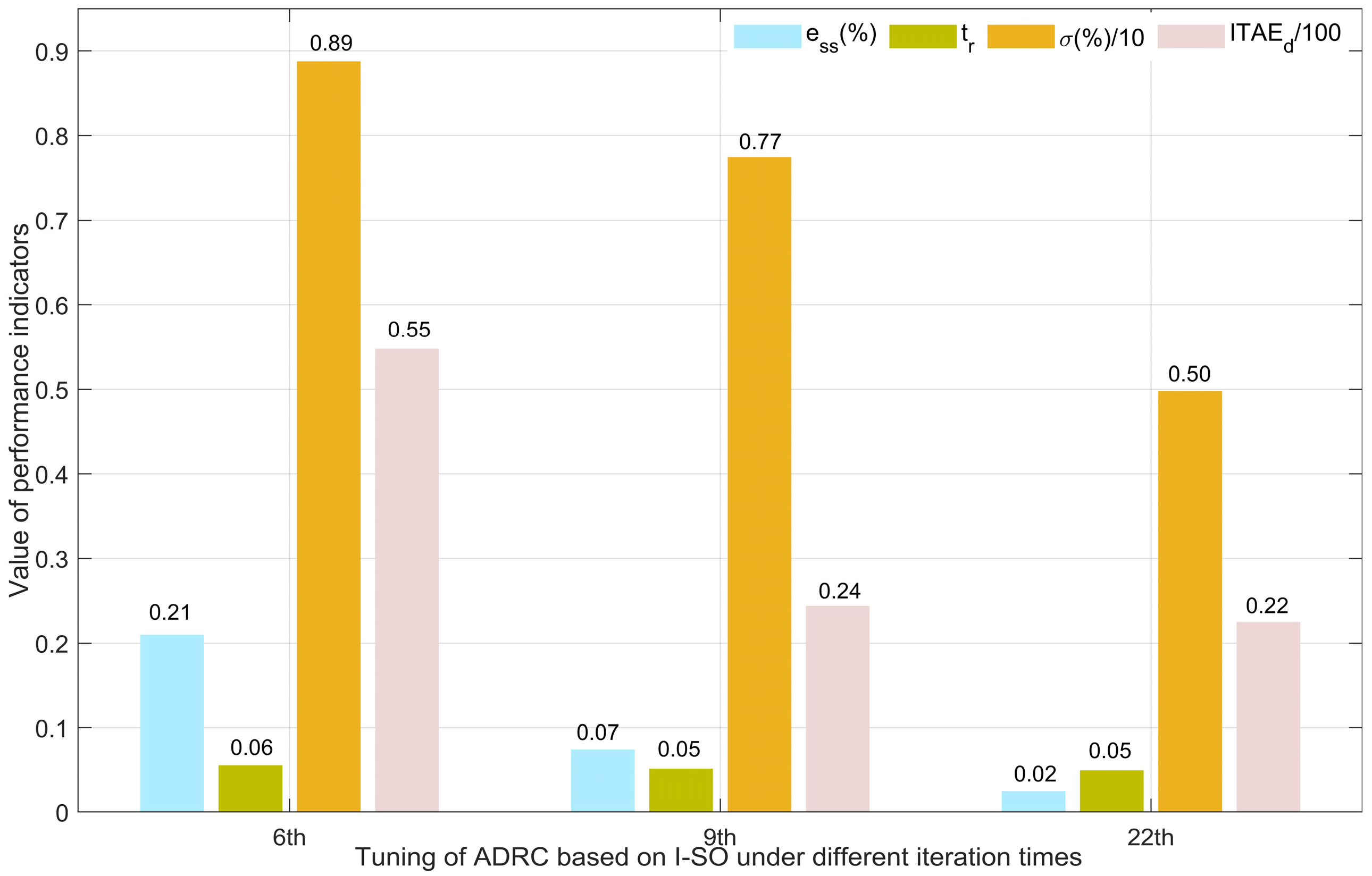
Table 3 shows the fitness values and the dynamic and stable control indicators of the three iterations.
Based on
Table 3 and
Figure 9, it can be seen that as the number of iterations increases, the performance of the system improves steadily, while the values of the indicators and fitness function generally decline, especially overshoot and
, with significant reductions. The parameter sets obtained for iterations 6, 9, and 22 are applied to the control system, respectively, and the system response and error curves are obtained, as shown in
Figure 10. It can be seen in
Figure 10 combined with
Table 3 that the performance of the control system using the parameter set obtained in iterations 6 and 9 is not ideal. Compared with iterations 6 and 9, the performance of the control system is much better when using the parameter set obtained in iteration 22, which is also the final optimal parameter set.
4.3. Comparison of I-SO–ADRC with SO–ADRC
The simulation results presented in
Figure 5 and
Figure 6 demonstrate that I-SO is feasible and effective for ADRC parameter tuning. In order to verify the advantages of the proposed I-SO in solving the parameter tuning problem of ADRC, under the same experimental environment and parameter conditions, the SO algorithm was used to tune the parameters of ADRC. The calculation of indicators adopted the method proposed in
Section 4.
Table 4 lists the indicators of the two SO algorithms.
Figure 11 depicts a broken-line chart of the indicators of the two SO algorithms corresponding to
Table 4.
Figure 12 shows the convergence curves of the two SO algorithms. It can be seen from
Table 4,
Figure 11 and
Figure 12 that many of the indicators of I-SO are better than those of SO. Compared with SO, although I-SO has more convergence iterations, its running time is shorter and its fitness value is smaller, which shows that I-SO has stronger optimization ability and is less likely to fall into local optimality. I-SO has a much smaller STD than SO, indicating that the stability of I-SO is excellent.
Figure 13 presents a column comparison chart of the four indicators that constitute the fitness function.
Figure 14 shows the error curves obtained by applying the optimal parameter set corresponding to the two algorithms to the control system. According to
Figure 13 and
Figure 14, two different SO algorithms can be applied to the parameter tuning of ADRC and provide ideal control, but the performance of the system when applying the I-SO is better.
Considering indicators of the control system and optimization algorithm comprehensively, compared with the SO algorithm, I-SO has the advantages of strong search ability, short running time, and good stability.
4.4. Comparison between I-SO–ADRC and PSO–ADRC, GA-ADRC and SSA-ADRC
To verify the effectiveness and superiority of I-SO compared to other intelligent optimization algorithms, three well-known optimization algorithms—PSO, GA, and SSA—were applied to the parameters tuning of ADRC, and the results were compared with those of I-SO.
In this experiment, if the final fitness was less than 100, the final solution was considered the global optimal solution. Otherwise, the final solution was considered the local optimal solution. Finally, the unique parameter settings of the three optimization algorithms were determined in this paper, as shown in
Table 5. Other parameters like population size, upper limit, and lower limit were the same as those of I-SO. The initial number of iterations was set to 30.
Table 6 is a comparison of the indicators of the three algorithms against I-SO. According to [
21], for evaluation of the performance of improved evolutionary algorithms, statistical tests are required. In this paper, we chose to use the Wilcoxon rank-sum test and conduct it at the 5% significance level. Assuming that I-SO is the best algorithm among the four, expressed as N/A, the p-values of the three algorithms can be obtained, as shown in
Table 6. The p-values of the three algorithms are less than 0.05, which shows that the superiority of the I-SO algorithm is statistically significant.
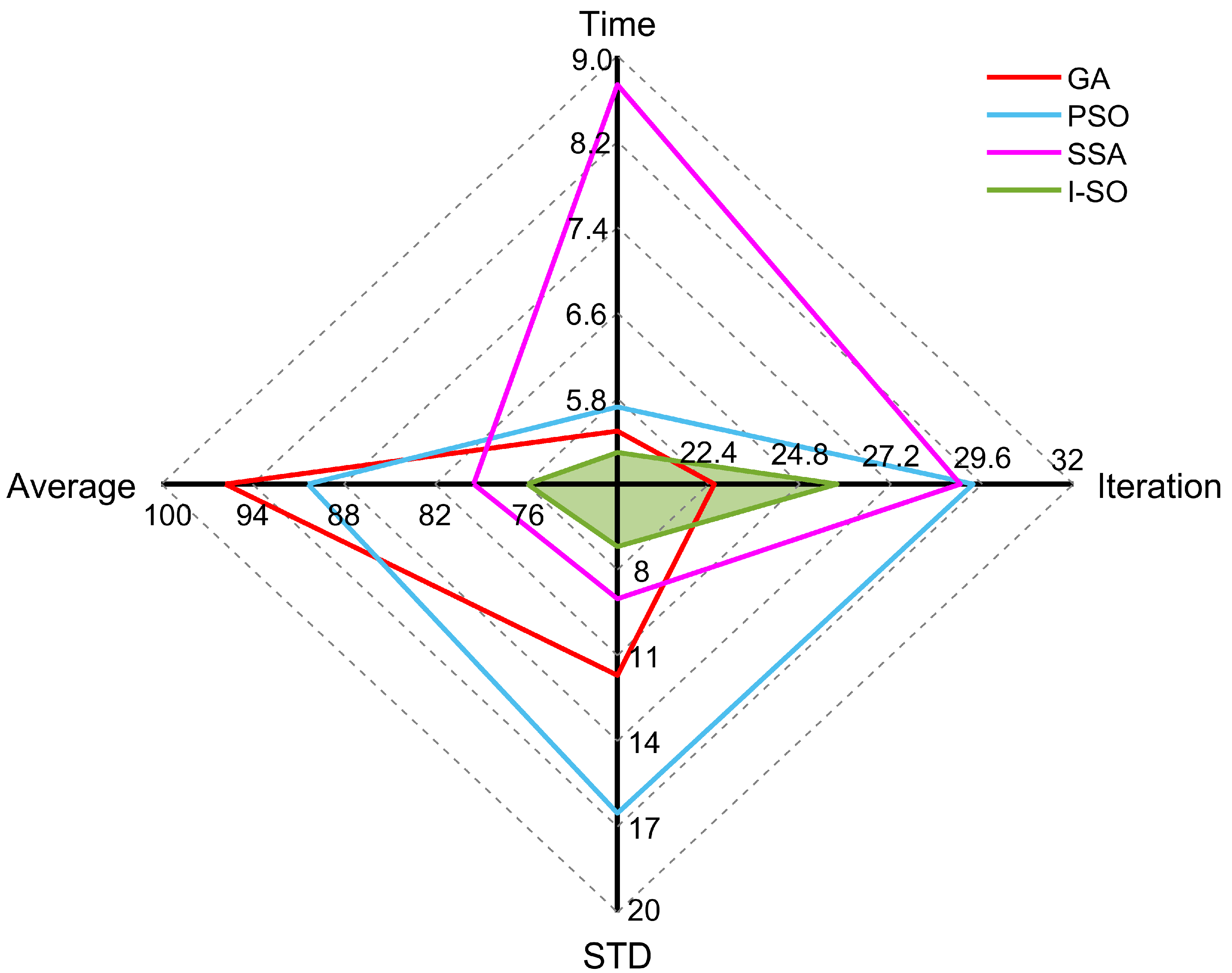
Figure 15 provides a radar map comparing the four algorithms, where the four axes, respectively, correspond to the four indicators in
Table 6. The quadrangles with different colors represent the different algorithms. As seen in
Figure 15, the green quadrangle representing the I-SO algorithm is almost completely encircled by the other quadrangles.
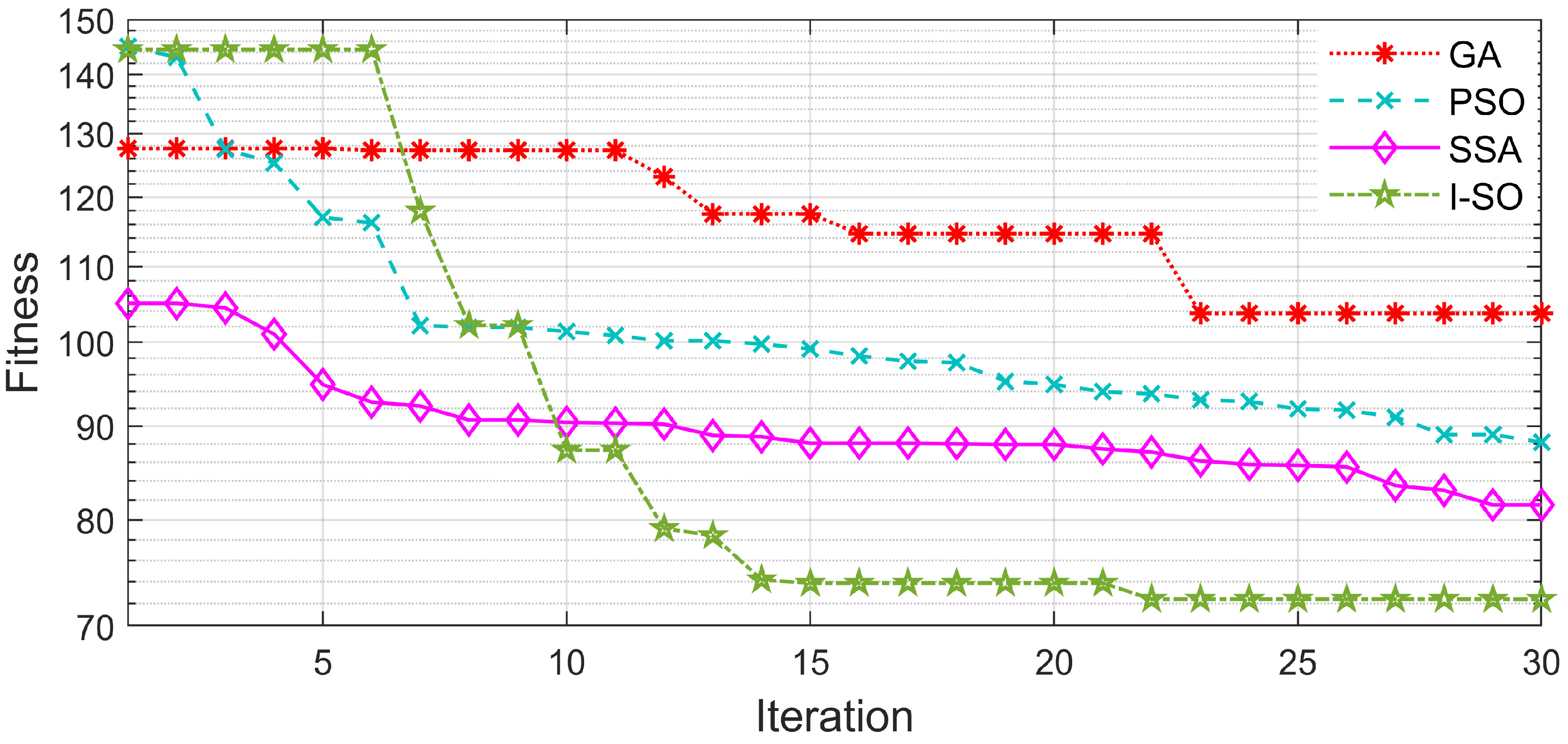
Figure 16 shows the convergence curves of the four algorithms. According to
Table 6,
Figure 15 and
Figure 16, among the four algorithms, the average, STD, and time of the I-SO algorithm are the smallest, and only the convergence speed is slightly higher than that of GA. Compared with the other three algorithms, I-SO has stronger search ability, better stability, faster convergence, and lower complexity.
Figure 17 exhibits columnar comparison charts of the four indicators constituting the fitness function.
Figure 18 shows the error curves obtained by applying the optimal parameter set corresponding to the four algorithms to the control system. According to
Figure 17 and
Figure 18, compared with SSA and GA, the control system corresponding to I-SO shows a more ideal control effect and several control indicators achieve smaller values. The control effect of the PSO-based system is also ideal. Compared with PSO, the I-SO algorithm is advantageous in its stability and disturbance observation ability. To sum up, the I-SO algorithm proposed in this paper can adjust ADRC parameters more effectively than the other three algorithms.
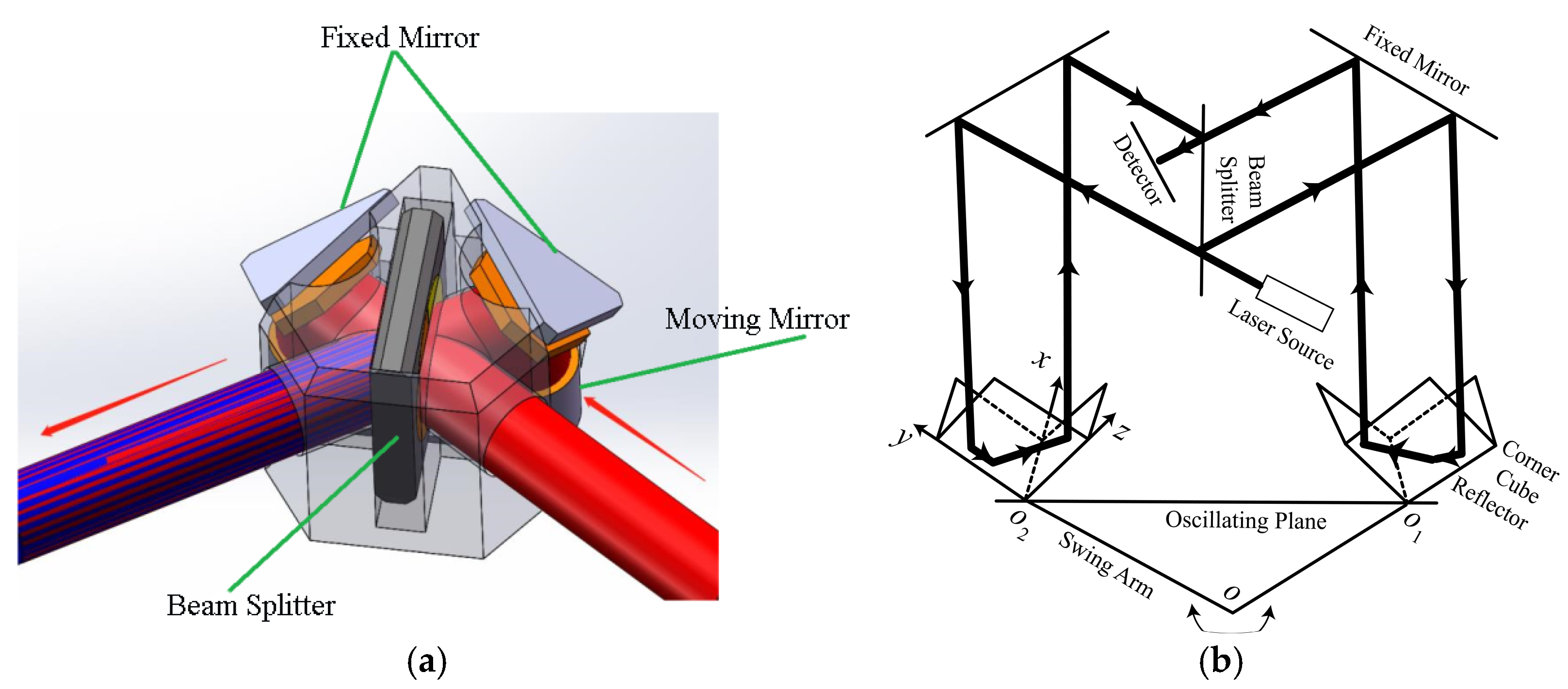
5. Moving Mirror Control System
For the swing-arm interferometer in
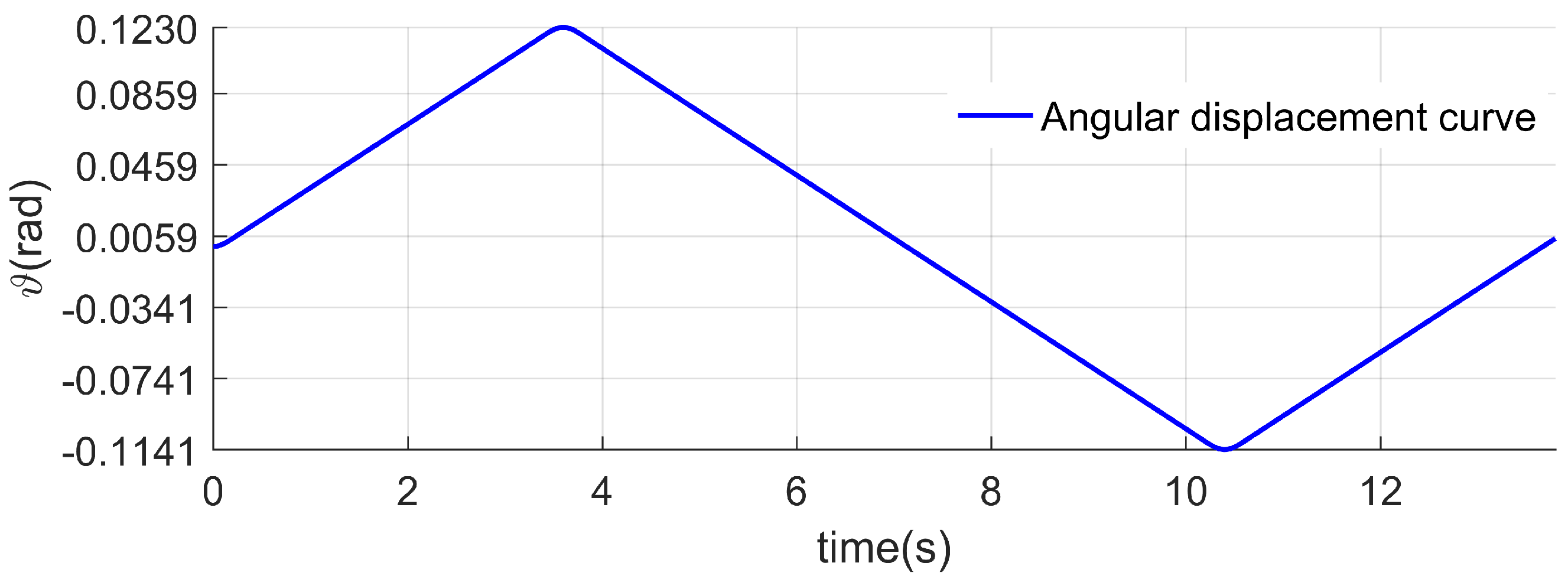
Figure 1, after derivation and a reference review, this paper obtained the equation of the swing angular displacement
of the RVCM and the optical path scanning speed
of the Fourier transform, as shown in Equation (28):
where
is the length of the swing arm. According to Equation (28) and the interferometer parameter,
,
, the motion curve of RVCM can be designed as shown in
Figure 19.
Saber and MAST languages were used to build the RVCM, H-bridge, and DSP models, a complete moving mirror control system was built, and joint simulation with Simulink 2022b was conducted to verify the effectiveness of ADRC with parameters tuned through I-SO. The simulation system is shown in
Figure 20. The controller uses the optimal solution obtained by the I-SO. Considering that an H-bridge is used in the system, the parameters of SEF may need to be modified. After debugging, the value of
is modified to 90. The parameters of LESO are not modified.
The simulation results are shown in
Figure 21 and
Table 7.
Table 7 shows the following error of the system. According to
Figure 21a and
Table 7, it can be seen that the maximum following error of angular displacement is 0.17 mrad, and large following errors appear during the starting and commutation stages of the RVCM.
In
Figure 21a, we can see that the curve experiences jittering, but the value of the jitter is extremely small, close to 0. There may be two reasons for the jitter shown in
Figure 21a: first, the simulation step size of the Saber 2019 in this paper may be set too low, which affects the simulation accuracy; second, the current loop in the simulation system may cause the simulation results to be unstable, causing the curve to jitter.
The following curve and error curve of the angular velocity are shown in
Figure 21b. It can be seen that large angular velocity following errors and fluctuations occur during the starting stage of the RVCM. However, during the steady-operation stage of the RVCM, the angular velocity following error is close to 0, achieving an excellent following effect. The stability of the optical path scanning speed of this system is calculated to be 99.2% in 4–10 s. The simulation results prove that the ADRC system tuned using I-SO has excellent control for the moving mirror control system and has a good following effect on the planned motion trajectory. Using I-SO to adjust the parameters of ADRC is efficient and effective, which provides certain reference significance for the use of the ADRC algorithm in moving mirror control systems.

 ,
, 


