Research on the Choice of Strategy for Connecting Online Ride-Hailing to Rail Transit Based on GQL Algorithm

Abstract

As traditional connection studies ignore the unbalanced distribution of connection demand and the variability of connection situations, this results in a poor match between passenger demand and connection mode, increasing passenger travel costs. Combining the economic efficiency of metro network operations with the unique accessibility advantages of ride-hailing services, this study clusters origin and destination points based on different travel needs and proposes four transfer strategies for integrating ride-hailing services with urban rail transit. Four nested strategies are developed based on the distance between the trip origin and the subway station’s service range. A reinforcement learning approach is employed to identify the optimal connection strategy by minimizing overall travel cost. The guided reinforcement learning principle is further introduced to accelerate convergence and enhance solution quality. Finally, this study takes the Fengtai area in Beijing as an example and deploys the Guided Q-Learning (GQL) algorithm based on extracting the hotspot passenger flow ODs and constructing the road network model in the area, searching for the optimal connecting modes and the shortest paths and carrying out the simulation validation of different travel modes. The results demonstrate that the GQL algorithm improves search performance by 25% compared to traditional Q-learning, reduces path length by 8%, and reduces minimum travel cost by 11%.

1. Introduction

With the development of the economy and advancements in Internet technology, the volume of ride-hailing services has been growing rapidly. Compared to public transportation, ride-hailing services have gradually become an important component of transportation services due to their advantages in convenience and accessibility. However, ride-hailing services also have the drawback of higher travel costs. As a result, some passengers opt for a hybrid travel model that combines the convenience of ride-hailing with the cost-effectiveness of public transportation. The most common example is the integration of metro and ride-hailing services. Therefore, how to effectively integrate ride-hailing services with urban rail transit to reduce travel costs for passengers, enhance travel convenience, shorten travel time, and build a green, friendly, and sustainable transportation system has become an urgent issue that needs to be addressed.

Existing multimodal transport optimization research mainly focuses on evaluation systems for transfers between different modes of public transport. The principal interchange modes that have been the subject of study are subway–bus, bus–bicycle, and subway–bicycle. The travel time for the connections is typically determined through network analysis, GIS software analysis of origin and destination points, and passenger flow data mining methods [1]. In terms of analyzing transfer paths, Liu [2] points out that accurately representing various urban transport networks and improving connections between transport networks are crucial for understanding travel behavior and enhancing the resilience of transport systems. Wu [3] developed a subway station spacing calculation model aimed at reducing passenger travel time by incorporating both grid and radial road network configurations, thereby improving the model’s applicability across various urban settings. Liu [4] applied a greedy triangulation algorithm to identify possible routes for intermodal transfers across different transportation modes, followed by the development of a multi-objective optimization framework aimed at reconciling sustainability with efficiency in multimodal transport, ultimately lowering travel expenditures.

Most of the traditional path optimization methods use heuristic search algorithms such as $A^{*}$ [5], genetic algorithms [6], and DQN algorithms. However, traditional genetic algorithms have some drawbacks in path planning problems, like long planning times, slow convergence, unstable solutions [7], and the possibility of getting stuck in local optima [8]. DQN algorithms also have some issues in path planning problems, like relatively low efficiency in action selection strategies and reward functions [9], long learning times, and slow convergence speeds [10]. As the problem scale increases, it becomes challenging to find the optimal solution within a constrained timeframe for medium- to large-scale instances, resulting in the attainment of only a local optimum. In recent years, reinforcement learning has gained attention since it addresses (model-free) Markov decision process (MDP) problems, where the system dynamics are not known, yet optimal policies can be derived from data sequences collected or generated under a specific strategy.

A substantial body of research has been carried out by researchers into the application of reinforcement learning for addressing path optimization problems, which can be classified into model-based and model-free approaches. One of the most representative algorithms for model-free methods is the Q-learning algorithm based on Markov decision processes [11]. Zhou [12] improved path planning efficiency by using a novel Q-table initialization method and applying root mean square propagation in learning rate adjustment. Wang [13] utilized the energy iteration principle of the simulated annealing algorithm to adaptively modify the greedy factor throughout the training process, thus improving the path planning efficiency and accelerating the convergence rate of the conventional Q-learning algorithm. Zhang [14] proposed an optimization framework based on multi-objective weighted Q-learning, using a positively skewed distribution to represent time uncertainty, which can solve multimodal transport multi-objective route optimization problems faster and better. Zhong [15] avoided the standard Q-learning algorithm falling into local optima by dynamically adjusting exploration factors based on the SA principle. Q-learning algorithms have been widely applied to path planning problems, but challenges such as the tendency to get stuck in local optima and slow convergence speed still exist, which are also current research hotspots.

Accordingly, this research, informed by residents’ travel demands and integrating the subway schedule along with the spatial and temporal characteristics of ride-hailing services, presents an investigation into optimizing short-distance ride-hailing connections to rail transit through the application of guided reinforcement learning techniques. Utilizing GPS data from online ride-hailing services in Beijing, this approach incorporates travel information extraction, road network modeling, cluster analysis, and connection route optimization. The Q-learning algorithm is applied to train the agent, and the guided reinforcement empirical principle is integrated to enhance learning efficiency and expedite the algorithm’s convergence rate. The most efficient path across various connectivity options is determined to minimize passenger travel expenses and shorten journey durations, thereby enhancing the attractiveness of public transportation and encouraging sustainable travel practices.

2. Problem Description

This study focuses on the travel decision-making for the combination of ride-hailing services and subway systems. This combined mode of transportation effectively integrates the wide coverage and high travel efficiency of ride-hailing services with the low-cost advantage of subway travel. It aims to ensure efficient passenger travel while increasing the attractiveness of subway systems and reducing overall travel costs and energy consumption. It aims to provide users with a more convenient, intelligent, and environmentally friendly travel experience.

Subways are the most convenient urban transportation mode. However, for parallel subway lines, passengers frequently need to make several transfers to arrive at their destinations, leading to increased travel distances and diminished transfer convenience. To maximize the benefits of subway systems, the “last mile” problem between subway stations and the final destinations needs to be addressed. As shown in Figure 1, traveling by subway alone takes a long time, and traveling by taxi is expensive. However, combining taxi services with the subway can effectively reduce travel costs for suburban residents and improve travel efficiency. It can also efficiently address the “last mile” challenge and alleviate the inconvenience of transferring between parallel subway lines.

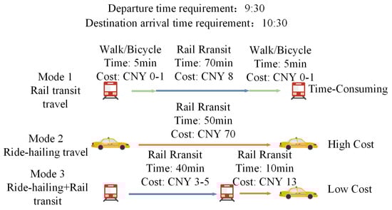
Figure 1. Comparison of travel modes.

To effectively integrate ride-hailing services and subway travel, this study first conducts cluster analysis and road network modeling using real data to identify pick-up and drop-off hotspots. Next, buffer zones are established around subway stations to analyze the connection modes for travel origins and destinations. Finally, a Guided Q-Learning (GQL) algorithm is proposed to search for the optimal connection mode and shortest path for travelers. Simulations are conducted to validate the proposed approach for different travel modes. The research findings and conclusions are presented in this study, as shown in Figure 2.

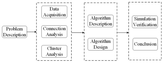
Figure 2. Technical route.

3. Materials and Methods

3.1. Methods of Data Acquisition and Analysis

The dataset employed in this research primarily comprises vehicle GPS records, real-world road network information, and subway line details. The vehicle GPS data was collected from ride-hailing services in Beijing, China, during a one-week period in June 2020 and spans the geographic region defined by longitudes 116°26′44″ to 116°33′76″ and latitudes 39°80′12″ to 39°84′95″ within the WGS-84 coordinate system. Since the obtained trajectory data is in the GCJ-02 coordinate system, which differs from the coordinate system of the OpenStreetMap (OSM) platform’s downloaded electronic map, Python 3.8 was used to convert the ride-hailing GPS data to the WGS-84 coordinate system to ensure consistency with the road network data. The road network file of Beijing was downloaded from the OSM platform. Then, the obtained road network data was filtered and clipped using the geospatial processing software QGIS. To ensure the accuracy of the road network, SUMO was used to depict the connectivity of roads and details of intersections. The established road network in this study is located in the Fengtai District of Beijing, comprising 241 nodes, 736 road segments, and 14 subway stations, as shown in Figure 3 and Figure 4.

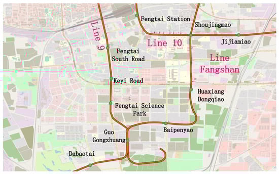
Figure 3. Actual road network.

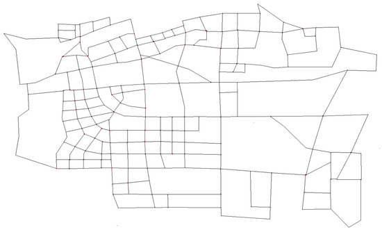
Figure 4. Road network modeling by SUMO.

3.2. Analysis of Connection Mode of Spatial Clustering

3.2.1. Connection Mode Analysis

To investigate suitable connectivity patterns for various origin–destination (OD) pairs, it is essential to examine the spatial arrangement between each OD location and the nearby subway stations. While walking is the predominant means of accessing subway stations, excessive distances may render walking insufficient for meeting travelers’ requirements. Consequently, the distance walked from the starting point to the subway station significantly affects passengers’ transportation decisions. This paper introduces an enhanced approach that segments the region into a circular buffer zone, centered at the entrance of each subway station, with the radius established according to the actual average distance between subway stations within the city. According to reference [16], a buffer radius of 500 m is chosen for the subway stations. The buffer setting are illustrated in Figure 5.

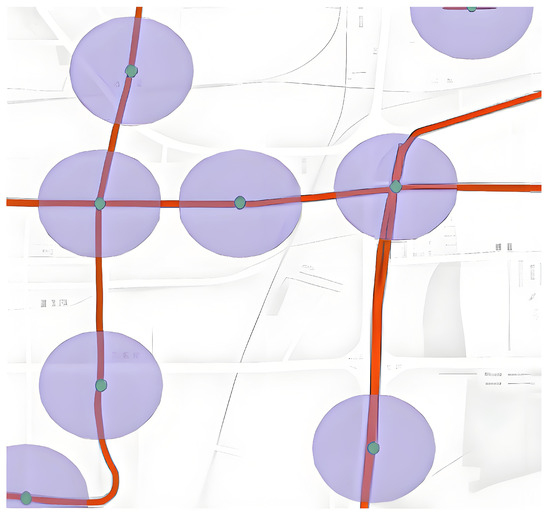
Figure 5. Buffer setting.

As the selected area involves parallel subway lines with a significant distance between them, the convenience of transfers is relatively poor. The proposed connection modes in this study can better address the “last mile” problem of subway travel. We extracted OD pairs within and outside the buffer zones, and based on Figure 6, the existing OD pairs are classified into the following four connection modes based on the spatial relationship between the origin and destination points and the buffer zones:

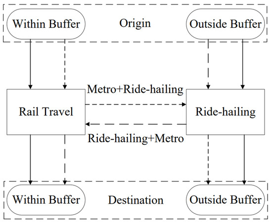
Figure 6. Connection mode division.

• MM (Metro–Metro) Travel Mode: If both the starting and ending locations fall within the designated buffer areas, it is advised to complete the entire trip using the subway system;
• MT (Metro–Taxi) Travel Mode: When the starting location is situated within the buffer zone and the ending location lies beyond the buffer zone, it is advisable to utilize a combination of metro and ride-hailing services, specifically by taking the metro first, followed by a ride-hailing service;
• TM (Taxi–Metro) Travel Mode: In cases where the starting location is situated outside the buffer zone and the endpoint lies within the buffer zone, it is advisable to utilize a combination of ride-hailing and subway services, specifically by using ride-hailing first, followed by the subway;
• TT (Taxi–Taxi) Travel Mode: When both the starting and ending locations are outside the buffer zones, it is recommended to travel the entire journey by ride-hailing services.

3.2.2. Spatial Cluster Analysis

This section examines the spatial and temporal distribution patterns of ride-hailing pick-up and drop-off locations, identifying areas with high-density concentrations, thereby offering a data foundation for the simulation example presented in the subsequent sections of this paper. The selected region is segmented into grid units, with data volume aggregated within each grid, and a heat map depicting passenger flow is presented in Figure 7. This heat map allows for the identification of areas characterized by a higher concentration of online ride-hailing activities and the spatial distribution of passenger movement. The depth of the color indicates the level of ridership: the dark color indicates the area with large ridership, and the light color indicates the area with lower ridership [17].

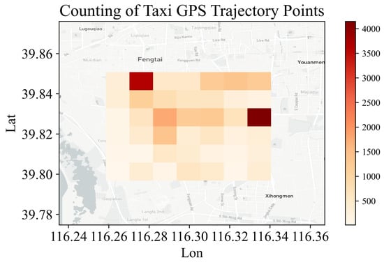
Figure 7. Statistical thermal map of passenger flow.

This study employs the K-means algorithm [18] to conduct cluster analysis on regions with high concentrations of drop-off and pick-up locations. The optimal number of clusters, represented by K, is identified through the application of the elbow method and the silhouette coefficient approach [19]. The clustering effectiveness is assessed using the CH index.

Based on the outcomes of SSE, CH, and SilScore presented in Figure 8, the ideal number of clusters for both origin and destination points is identified as 8. The cluster configurations and corresponding passenger flow data for each cluster are displayed in Figure 9 and Figure 10, respectively. The research area is divided into residential and work areas. Clusters 0 to 4 have a higher passenger flow. The hotspots for drop-off and pick-up points of ride-hailing passengers are closely related to their geographical locations. Areas with complex socio-economic activities tend to have a higher density of ride-hailing usage. For example, passengers in Cluster 0 are located near the Fengtai Science and Technology Park, which has higher commercial activity and a greater demand for travel. On the other hand, areas with predominantly residential activities have a lower density of ride-hailing usage. For example, passengers in Cluster 5 are located near the Yurenli residential area, where travel demand is relatively low. Based on the results, these eight cluster centers (location points) are considered as the hotspots for ride-hailing demand. The latitude and longitude information of these centers are provided in Table 1.

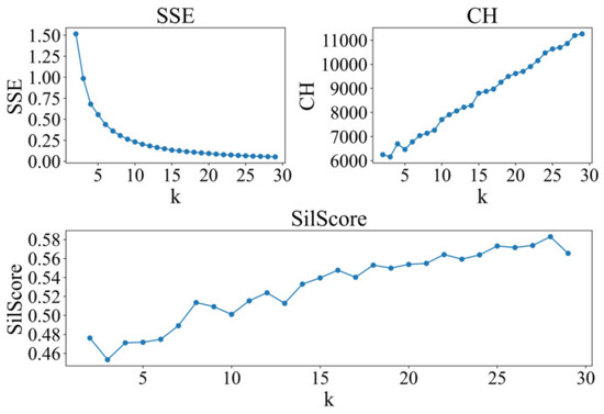
Figure 8. K-means index.

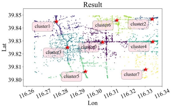
Figure 9. Clustering result.

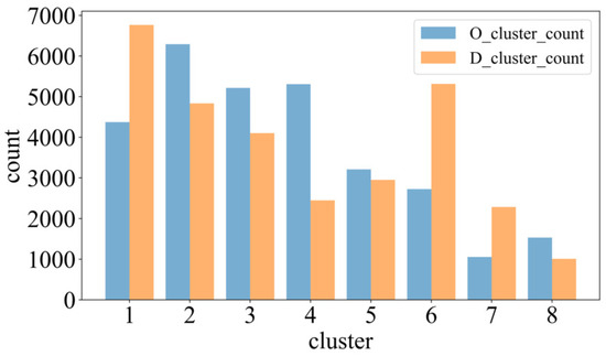
Figure 10. Passenger flow statistics of each cluster.

Table 1. Location information of the inbound and outbound hotspot OD.

OD	1	2	3	4	5	6	7	8
Inbound longitude	116.288	116.335	116.313	116.295	116.278	116.306	116.33	116.334
Inbound latitude	39.8251	39.8293	39.8461	39.8067	39.845	39.8291	39.8077	39.847
Outbound longitude	116.284	116.315	116.278	116.331	116.334	116.295	116.306	116.335
Outbound latitude	39.8258	39.8458	39.845	39.8077	39.8286	39.8257	39.8289	39.847

3.3. Travel Cost Definition

3.3.1. Travel Time

Travel duration represents a critical element in assessing the efficiency of passenger transportation, encompassing walking time, waiting time, and in-vehicle time, along with an error adjustment to enhance the precision of the computation.

1.

Walking time

Walking time encompasses the duration required for passengers to travel on foot from their starting location to the departure station, the time needed to move between consecutive boarding points during transfers, and the time spent walking from the arrival station to the final destination or designated pickup location for ride-hailing services.

$$\begin{array}{c}\hfill {\mathrm{T}}_{\mathrm{in}}={\displaystyle \frac{S_O}{V_w}}.\end{array}$$

(1)

$$\begin{array}{c}\hfill {\mathrm{T}}_{\mathrm{transfer}}={\displaystyle \frac{S_{transfer}}{V_w}}.\end{array}$$

(2)

$$\begin{array}{c}\hfill {\mathrm{T}}_{\mathrm{out}}={\displaystyle \frac{S_D}{V_w}}.\end{array}$$

(3)

where $T_{in}$ denotes the walking time from the origin to the departure station, $T_{transfer}$ denotes the walking time between boarding points during transfers, and $T_{out}$ denotes the walking time from the destination station to the destination. Additionally, $S_O$ denotes the walking distance from the origin to the departure station, $S_{transfer}$ denotes the walking distance during transfers, and $S_D$ denotes the walking distance from the destination station to the destination. $V_w$ denotes the average walking speed of the passengers.

2.

Waiting time

The passenger’s waiting time encompasses the duration spent awaiting the arrival of a train or the pickup by a ride-hailing vehicle. In this study, it is assumed that the arrival time intervals for vehicles are fixed [20], and the passengers’ arrivals follow a uniform distribution.

$$\begin{array}{c}\hfill {\mathrm{T}}_{\mathrm{wait}}={\displaystyle \frac{H_k}{2}}+300.\end{array}$$

(4)

where $H_k$ represents the average departure interval time for trains on line k, measured in seconds. The waiting time for a ride-hailing vehicle to pick up a passenger is assumed to be a uniform 5 min (300 s) for all cases.

3.

Travel time

The duration of rail transit travel denotes the period passengers spend within a subway station, encompassing both the time trains are in motion and the time they remain stationary. Typically, the travel duration between stations remains constant and can be established according to the train timetable. The travel time for rail transit is denoted as $T_m$:

$$\begin{array}{c}\hfill {\mathrm{T}}_{\mathrm{m}}={\displaystyle \frac{S_m}{V_m}}+t_{stop}.\end{array}$$

(5)

The travel time for ride-hailing includes the time spent by the cars driving on the road network. The travel time for different time periods can be considered as an attribute and incorporated into the road segment properties. It can be obtained through querying services like Google Maps. The travel time for ride-hailing is denoted as $T_t$:

$$\begin{array}{c}\hfill {\mathrm{T}}_{\mathrm{t}}={\displaystyle \frac{S_{i,j}}{V_{i,j}}}.\end{array}$$

(6)

where $S_m$ and $V_m$ are the distance and speed of the metro taken by passengers, $t_{stop}$ is the stop time of the metro, and $S_{i,j}$ and $V_{i,j}$ are the driving distance and driving speed of the i-j section of the road network, respectively.

4.

Total travel time

The travel time cost includes the unit time value (unit time cost) and the total travel time. In the context of urban rail transit connecting with ride-hailing car travel mode, the travel time cost is represented as follows:

$$\begin{array}{c}\hfill {\mathrm{T}}_{\mathrm{all}}=(T_{in}+T_{transfer}+T_{out}+T_{wait}+T_m+T_t+T_{error}).\end{array}$$

(7)

Due to the randomness of the total travel time, the factor $T_{error}$ is introduced to ensure the accuracy of the solution.

3.3.2. Travel Cost

The subway travel fare in Beijing, China, is calculated using a segmented pricing system, and the expression is as follows:

$$\begin{array}{c}\hfill {\mathrm{C}}_{\mathrm{M}}=\left\{\begin{array}{c}3,0<S_M\le 6\hfill \\ 4,6<S_M\le 12\hfill \\ 5,12<S_M\le 22\hfill \\ 6,22<S_M\le 32\hfill \\ 6+(32-S_M)/20,S_M>32.\hfill \end{array}\right.\end{array}$$

(8)

where $S_M$ is the distance of subway travel in kilometers and $C_M$ is the subway travel fare in Chinese yuan.

The travel cost of a ride-hailing vehicle includes the initial fee, fuel surcharge, and an additional cost for exceeding the initial distance. The expression is as follows:

$$\begin{array}{c}\hfill {\mathrm{C}}_{\mathrm{T}}=\left\{\begin{array}{c}14+1.8\times S_d+0.8\times T_d,6\le T_{\xi }\le 10\hfill \\ 13+1.45\times S_d+0.4\times T_d,10\le T_{\xi }\le 17\hfill \\ 13+1.5\times S_d+0.8\times T_d,17\le T_{\xi }\le 21\hfill \\ 14+2.5\times S_d+0.8\times T_d,21\le T_{\xi }\le (+1)6.\hfill \end{array}\right.\end{array}$$

(9)

where $S_d$ represents the distance traveled by a ride-hailing vehicle beyond the initial distance in kilometers, $T_d$ represents the travel time of a ride-hailing vehicle in seconds, and $C_T$ represents the total travel cost of a ride-hailing vehicle in yuan. $T_{\xi }$ represents the discrete time variable.

$$\begin{array}{c}\hfill {\mathrm{C}}_{\mathrm{F}}=C_M+C_T.\end{array}$$

(10)

where $C_F$ represents the total cost of the rail connection to an online ride-hailing trip.

4. Guided Q-Learning Algorithm

4.1. Q-Learning Algorithm Overview

Q-learning (QL) is a reinforcement learning algorithm that operates without a model. Model-free refers to the fact that the agent has no information about the environment and needs to interact with the environment to collect a lot of trajectory data. The agent obtains information from the trajectory to improve the strategy and obtain more rewards [21]. It consists of three main components: Q-table initialization, action selection policy, and Q-table update. Through repeated interactions between the agent and the environment, the agent learns and acquires one or a series of optimal behaviors. This learning procedure is implemented as a Markov decision process (MDP), as illustrated in Figure 11.

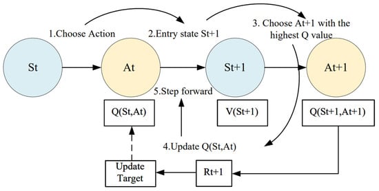
Figure 11. Markov decision process.

An MDP is represented by a tuple $(S,A,P,R)$, where S denotes a finite collection of states, A represents the set of actions accessible to the agent, P signifies the transition probability function, and R indicates the reward function. The anticipated reward associated with a specific state–action pair $(s,a)$ is expressed as follows:

$$\begin{array}{c}\hfill \mathit{R}(\mathit{s},\mathit{a})=\sum _{s^{\prime }\in S}p(s,a,s^{\prime })R(s,a,s^{\prime }).\end{array}$$

(11)

$Q(s,a)$ is a state–action pair and its corresponding reward value. Following the update strategy, the revised Q values can be derived by solving the linear system formed by Bellman’s equation, reflecting the Q values associated with each operation that could be executed immediately.

$$\begin{array}{c}\hfill {\mathrm{Q}}^{*}({\mathrm{s}}_{\mathrm{t}},{\mathrm{a}}_{\mathrm{t}})=Q(s_t,a_t)+\alpha \left[r_t+\gamma \underset{a^{\prime }}{max\left(Q(s_t,a^{\prime })\right)}-Q(s_t,a_t)\right].\end{array}$$

(12)

where $\alpha$ denotes the learning rate and $\gamma \in (0,1)$ is the attenuation factor of future reward. For every Markov decision process, there exists an optimal deterministic strategy that maximizes the total expected reward from the initial state to the target state.

4.2. Algorithm Design

The algorithm designed in this paper focuses on the road network, where the nodes represent road intersections and the actions represent the selection of the next node. Both the state set and the action set are finite. The Temporal Difference (TD) learning algorithm can directly interact with the environment and learn from sampled data obtained during the interaction. Q-learning, as one of the classic TD learning algorithms, is highly applicable in this context.

Drawing upon the foundations of the Markov decision process and Q-learning and Sarsa algorithms, this study introduces the GQL algorithm. Grounded in a real-world road network, the algorithm develops a topological representation of the network, which functions as the search space and establishes an allowable set of actions for each OD pair. The algorithm identifies the most suitable transportation mode for any given origin–destination pair by analyzing the spatial information of both locations, subsequently determining the most efficient route and making travel decisions accordingly. The primary principle guiding the selection of the transportation mode involves locating the closest metro station to both the origin and destination. Taking into account the catchment area of each metro station, the algorithm prioritizes and suggests more cost-effective travel alternatives where feasible.

When the algorithm identifies various modes of transportation, it applies tailored reward mechanisms accordingly. By utilizing an $\epsilon$-greedy strategy informed by the chosen action for the current state, the algorithm adheres to the principle of guided reinforcement learning, incorporating the “nearest subway station” as a guiding element to progressively identify the optimal route within the selected transportation mode. The ultimate result encompasses the route distance, means of conveyance, and most efficient path for the specified origin–destination pair. The procedural outline of GQL is presented in Algorithm 1.

Algorithm 1: GQL

Establish a road network model

Determine the attraction range of each subway station

Get the travel information of the hot boarding and unloading area

Build the optional action set and initialize the environment,

Initialize parameters: $\alpha$, $\gamma$, $\epsilon$, p

Initialize the starting and ending points: $S_{begin}$, $S_{end}$

for sequence e = 1 → E do: (for each turn loop)

Get initial state s

for step t = 1 → T do:

according to $S_{begin}$ and $S_{end}$, get mode =‘MM’/‘TM’/‘MT’/‘TT’

Set up the reward mechanism for different connection modes

Select Action a in current s based on $\epsilon$-greedy policy

Perform a, get the environment feedback r, $S_{t+1}$, calculate r

Add experience (s, a, r, s’) to the experience pool buffer

Choose a random e = (s, a, r, s’) and the target state g

Generate new experience e’ = (s, a, r’,g)

Add e’ to buffer

Sample experience Q from buffer in order of priority

Adopt the update principle of Sarsa to update Q table:

$Q(s_t,g,a_t)=Q(s_t,g,a_t)+\alpha \left[r_t+\gamma \underset{a^{\prime }}{maxQ(s_{t+1},g,a^{\prime })}-Q(s_t,g,a_t)\right].$

S ← $S_{t+1}$

If the new state is the target state, give a special reward signal

Calculate the cumulative reward, path length, and learning time

end for

end for

Output optimal path, connection mode, path length

4.2.1. Status

The actual road network is abstracted into a topological structure based on the real-world road layout, as illustrated in Figure 12. In this representation, road junctions and subway stops are modeled as nodes. The road system is formalized as a directed graph $G=(J,E,W)$, where J denotes the set of nodes corresponding to road intersections and subway stations, E signifies the directed edges linking these nodes, and W indicates the actual distance between adjacent nodes.

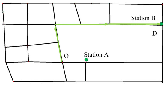
Figure 12. Road network topology.

The subsequent assumptions pertain to the nodes within the road network and the lengths of the road edges, which are static attributes in an undirected graph structure:

• Each roadway permits access and departure for ride-hailing services at both terminal points of the node;
• Distances required for executing left turns, right turns, proceeding straight, or turning around are minimal and may be disregarded;
• When a ride-hailing vehicle begins its journey from any location along a roadway, the starting point is designated as the nearest road network node to that location [22]. In Figure 13, nodes A and B illustrate road network nodes, while point C indicates the passenger’s pickup location or the vehicle’s initial position. $L_1$ denotes the actual distance between C and A, whereas $L_2$ represents the actual distance between C and B. If $L_1$ > $L_2$, the passenger or ride-hailing vehicle’s location is considered to be at node A.
  

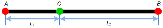  Figure 13. Select the source or destination node.

The agent’s state is characterized by the collection of nodes available for selection within the road network.

$$\begin{array}{c}\hfill \mathit{S}=\{J_0,J_1,\dots ,J_n\}.\end{array}$$

(13)

where $J_i$ represents a road node in the road network.

4.2.2. Action

Actions refer to the collection of permissible moves available to the agent in a particular state, indicating the potential maneuvers a vehicle may perform at each intersection. In this study, the four possible actions for a vehicle at a particular state are defined as follows: left turn, right turn, straight ahead, and turn around. It is presumed that, when the agent is located at any given road node, it has the capability to choose the subsequent connected intersection as its next move [23]. The collection of possible actions at each node is specified as follows:

$$\begin{array}{c}\hfill \mathit{A}=\left\{J_i:\left[i\to i_1,\dots ,i\to i_k\right]\right\}.\end{array}$$

(14)

where $J_i$ denotes the agent’s state and $i_k$ refers to the adjacent nodes associated with state $J_i$. The integration of states and actions constitutes the agent’s environment.

4.2.3. Action Selection Policy

In the QL algorithm, each state–action pair is associated with a corresponding Q value, and one approach to selecting actions is to pick the one with the maximum Q value. Nevertheless, this method has drawbacks, as it does not guarantee optimal long-term results and prevents the agent from exploring potentially superior actions. To improve the agent’s exploration capabilities in unfamiliar environments, this study employs an $\epsilon$-greedy strategy for action selection. This approach addresses the exploration–exploitation dilemma by assigning probabilistic preference to both exploration and exploitation. Additionally, a noise term is added to the selected action at each step, and this noise decreases over iterations. The subsequent action is selected with probability $\epsilon$, while the action associated with the highest estimated expected reward, derived from prior experiences, is chosen with the complementary probability.

$$\begin{array}{c}\hfill {\mathrm{a}}_{\mathrm{t}}=\left\{\begin{array}{c}argma{x}_{a\in A}Q\left(a\right),p:1-\epsilon \hfill \\ \mathrm{random}\_\mathrm{choose},p:\epsilon .\hfill \end{array}\right.\end{array}$$

(15)

$$\begin{array}{c}\hfill \mathrm{noise}={\displaystyle \frac{r}{i+1}}.\end{array}$$

(16)

where $Q\left(a\right)$ represents the estimated reward value, $\epsilon$ represents the greedy coefficient, r represents a random number, and i represents the iteration count.

When the current environmental feedback yields a high reward, the effective state—specifically, the return value reduction algorithm—operates within a localized optimization range. To prevent entrapment in local optima and sustain efficient exploration, the algorithm must enhance its exploratory effectiveness. Therefore, on the basis of the stage optimization of the exploration step length, an exploration factor adjusted in real time according to the environmental return state can be added.

$$\begin{array}{c}\hfill \epsilon ={\displaystyle \frac{\epsilon }{1+lg(\lambda N\mathsf{\Delta }x/2x)}}.\end{array}$$

(17)

where $\epsilon$ represents the greedy coefficient, $\lambda$ represents the decay coefficient, set to 10 to ensure a negative correlation between exploration efficiency and environment reward status, $\mathsf{\Delta }x$ represents the effective reward status for compensating exploration in a particular phase, and N represents the total number of steps.

4.2.4. The Principle of Guided Experience

Directional information not only serves as part of the reward function but also guides the agent’s actions in the next state. If the direction tends towards the target point in one state, it is likely that the action in the next state will also tend towards the target point. Building on the standard QL algorithm, this study introduces a target state g. For scenarios MT and TM involving subway transportation, the nearest subway station is defined as an additional target state point. Special reward signals are used to guide the agent’s learning towards the target state, reducing the overall search scope, shown as Figure 14. By optimizing the agent’s action selection based on directional information, this approach adheres to the guided reinforcement empirical principle [24].

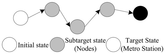
Figure 14. Target state.

The Replay Buffer is an experience principle used in GQL. It involves storing the agent’s experiences $(s_t,a_t,r_t,s_{t+1})$ in a buffer, where experiences can come from actions taken under different policies. Building upon the guided reinforcement empirical principle, this study randomly selects an experience $e=(s,a,r,s^{\prime })$ and a target state g to generate a new $e^{\prime }=(s,a,r^{\prime },g)$. Once the buffer is full, old experiences are replaced. During the training process, a sample experience is drawn from the buffer and used to update the agent’s Q value function. This approach has several advantages: it reduces the number of interactions with the environment by reusing past action experiences, which can save time during the training process, improves generalization performance, and leads to better training outcomes.

4.2.5. Reward Function

Because the QL algorithm is based on the Markov decision process (MDP) framework, the agent engages with the environment repeatedly, consistently obtaining feedback. This feedback is used to guide the agent in optimizing its behavior. To accomplish this, a reward function may be established to represent the utility obtained by the agent in each state, enabling the evaluation of favorable or unfavorable reinforcement for its actions. In different transfer modes, following the guided reinforcement empirical principle, the rewards from the various environments. The reward function is defined as follows:

$${\mathrm{R}}_{\mathrm{TO}}={\mathrm{R}}_{\mathrm{MT}}=\left\{\begin{array}{c}{r}_1,S_{next}=S_{end}\hfill \\ \mu r_1,S_{next}\ne S_{end},d_{next}<d_{now}\hfill \\ \mu r_2,S_{next}\ne S_{end},d_{next}>d_{now}.\hfill \end{array}\right.$$

(18)

$$\begin{array}{c}\hfill {\mathrm{R}}_{\mathrm{TM}}=\left\{\begin{array}{c}{r}_1,S_{next}=S_{nearest\_station}\hfill \\ \mu r_1,S_{next}\ne S_{nearest\_station},d_{next}<d_{now}\hfill \\ \mu r_2,S_{next}\ne S_{nearest\_station},d_{next}>d_{now}.\hfill \end{array}\right.\end{array}$$

(19)

where $R_{TT}$ denotes the reward function for the TT transfer mode, $R_{MT}$ represents the reward function for the MT transfer mode, $R_{TM}$ indicates the reward function for the TM transfer mode, $S_{next}$ refers to the agent’s subsequent state, $S_{end}$ signifies the terminal state of the journey, $d_{now}$ denotes the distance from the current location to the destination, and $d_{next}$ represents the distance from the next state location to the destination. $\mu$ is the reward transfer coefficient, ranging between 0 and 1, employed to assess the significance of the current reward, and $r_1$ denotes a positive constant indicating the positive reward magnitude, while $r_2$ signifies a negative constant reflecting the negative reward magnitude.

4.2.6. Update Rule

Based on the guided reinforcement empirical principle, this paper introduces the experience factor g and adopts the update principle of the Q-learning algorithm to update the Q table. The update mechanism is as follows:

$$\begin{array}{c}\hfill \mathrm{Q}({\mathrm{s}}_{\mathrm{t}},\mathrm{g},{\mathrm{a}}_{\mathrm{t}})=Q(s_t,g,a_t)+\alpha \left[r_t+\gamma \underset{a^{\prime }}{maxQ(s_{t+1},g,a^{\prime })}-Q(s_t,g,a_t)\right].\end{array}$$

(20)

where $Q(s_t,g,a_t)$ denotes the Q value of the current state, target, and selected action, $\underset{a^{\prime }}{Q(s_{t+1},g,a^{\prime })}$ represents the Q value associated with the subsequent state, updated target, and executed action, $\alpha$ signifies the learning rate, and $\gamma$ indicates the attenuation factor.

5. Numerical Simulation

5.1. Simulation Analysis

This study uses the real-world road network surrounding Fengtai Science Park in Beijing, China, to demonstrate the algorithm’s effectiveness. This road network consists of 241 intersections, 14 subway stations, and 736 road sections. The established environment of the agent is as follows. Example descriptions of GPS data are shown in Table 2.

Table 2. GPS data example description.

Field Name	Data Type	Data Length	Note
dateid	varchar	8	date of uploading location point information
time	varchar	6	time to upload location point information
licenseplate	str	5	licence plates of vehicles
carid	int	6	vehicle id
lon	numeric	8	longitude, rounded to six decimal places
lat	numeric	9	latitude, rounded to six decimal places
speed	numeric	3	traveling speed in m/s
direction	int	3	direction angle, with due north at 0 degrees, increasing in clockwise order
loaded	int	1	passenger carrying state

5.1.1. Impedance Matrix

In the matrix of Table 3, the numbers 0 to 240 represent 241 road nodes. Each segment of the road is two-way and of uniform length. The value between two nodes denotes the actual distance separating them. For example, the distance from node 0 to node 1 and from node 1 to node 0 is identical at 130.6 units. The diagonal entries are all zero, reflecting the absence of distance between identical nodes. Numerous entries marked as “inf” imply that the separation between certain nodes is infinite, indicating that no direct path exists between them. For example, if the distance from node 0 to node 3 is assigned a value of “inf”, this signifies that no viable path exists between these two nodes.

Table 3. Impedance matrix.

	0	1	2	3	…	239	240
0	0	131	inf	inf	…	inf	inf
1	131	0	134	632	…	inf	inf
2	inf	134	0	Inf	…	inf	inf
3	inf	inf	632	0	…	inf	inf
…	…	…	…	…	0	…	…
239	inf	inf	inf	inf	…	0	inf
240	inf	inf	inf	inf	…	inf	0

5.1.2. Optional Action Set for Each Node

In the configuration presented in Table 4, each node is able to select the adjacent junction as its subsequent action. Points with an effective distance between them in the road network impedance matrix can be connected to each other; that is, if there is an effective action, such as point J1, then J0, J2 and J65 can be selected as the next action.

Table 4. Optional action.

State	Optional Action
J0	J0 → J1, J0 → J64
J1	J1 → J0, J1 → J2, J1 → 65
J2	J2 → J1, J2 → J3, J2 → J67, J2 → J68
J3	J3 → J2, J3 → J4
…	…
J239	J239 → J101, J239 → J112
J240	J240 → J83, J239 → J115

5.1.3. Nodes Within Range of a Subway Station

The road network in this study includes a total of 14 subway stations in Table 5, with coordinates set as default in SUMO. After setting the buffer zone, each subway station has an attraction range of 500 m. There are a total of 73 road nodes located within the buffer zones.

Table 5. Nodes within the range of buffers.

ID	Station Coordinates	Range of Attraction	Optional Action Set
St1	Baipenyao (489.29, −957.83)
St2	Caoqiao (3758.88, 1456.93)
St3	Fengtao (−242.03, 1841.83)	500 m	J35, J41, J216, J221, …, J210, J211
…	…
St17	Dabaotai (−1464.22, −2064.39)

5.2. Instance Analysis

According to the clustered hotspots of passenger pick-up and drop-off areas, it can be inferred that the following road segments are hotspots for drop-off and pick-up points: Keji Avenue, Fengke Road, Nansihuan West Road, Fengtai East Road, Nansanhuang West Road, Huangchen Road, Fengtai East Road, Fangfei Road, and Fengtai Grand Bridge. These road segments are surrounded by a large number of points of interest, and points of interest within the same cluster have similar travel characteristics. We have selected four sets of hotspot OD pairs for the case study, as shown in Figure 15. We conducted experimental analysis using three different values of $\alpha$. The findings indicated that with $\alpha$ = 0.05, the agent demonstrated optimal convergence with respect to reward values, path length, and learning duration. The experimental setup included $\alpha$ = 0.05, $\gamma$ = 0.9, $\epsilon$ = 0.9, and episode = 200.

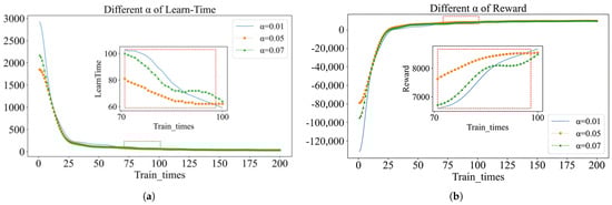
Figure 15. Parameter selection. (a) Different $\alpha$ of Learn-time. (b) Different $\alpha$ of reward.

5.2.1. MM Travel Mode

For MM travel mode in Table 6, that is, the starting points of passengers’ travel are within the range of subway attraction, the QL algorithm recommends passengers to take the subway for the whole journey, searches out the subway station closest to the starting point of passengers, and outputs the optimal subway transfer route. However, the QL algorithm only finds the online ride-hailing route without considering the subway line. In comparison, the GQL algorithm has stronger applicability. The dotted lines in Figure 16 represent the subway routes, which are shown in the table.

Table 6. MM travel mode.

MM Mode	O1	D1
Nodes	44	225
Distance to station	404.143	313.604
Station name	Jijiamiao	Guogongzhuang
Optimal path	44 > Jijiamiao (10) > Shoujingmao > Shoujingmao (Fangshan) > Huayuandongqiao > Baipenyao > Guogongzhuang > 225
Path length	5900
Price	6

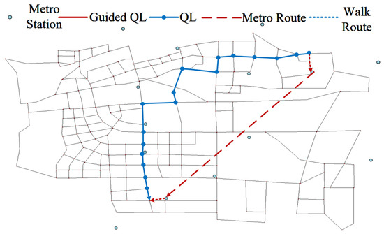
Figure 16. MM travel path.

5.2.2. TM Travel Mode

For the TM travel mode presented in Table 7, in cases where the passenger’s origin lies outside the subway station’s attraction range while the destination is within it, the GQL algorithm suggests using a ride-hailing service to link with the subway for the trip. The passenger would first travel via ride-hailing to Fengtai East Street Station, then proceed by subway to Baipenyao Station, and ultimately reach the destination on foot, as indicated by the dashed line in Figure 17.

Table 7. TM travel mode.

TM Mode	O2	D2
Nodes	4	210
Distance to station	2504.273	466.251
Station name	Fengtaidongdajie	Baipenyao
Optimal path	4 >Fengtaidongdajie (9) > Guogongzhuang > Baipenyao (Fangshan) > 210
Path length	6687.11
Price	19

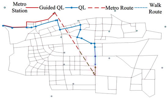
Figure 17. TM travel path.

5.2.3. MT Travel Mode

For the MT travel mode in Table 8, when the passenger’s departure point is within the attractive range of the subway station but the destination is beyond this range, the GQL algorithm suggests that the passenger first takes the subway and then completes the remaining journey through a ride-hailing car. Passengers will first walk to Caoqiao Station, then take the subway to Dabaotai Station, and finally reach their destination by ride-hailing car, as illustrated by the dashed line in Figure 18.

Table 8. MT travel mode.

MT Mode	O3	D3
Nodes	41	12
Distance to station	352.705	2364.433
Station name	Caoqiao	Dabaotai
Optimal path	41 > Caoqiao (10) > Shoujingmao > Dabaotai (Fangshan) > 20 > 19 > 18 > 17 > 16 > 15 > 14 > 13 > 12
Path length	8546.951
Price	19

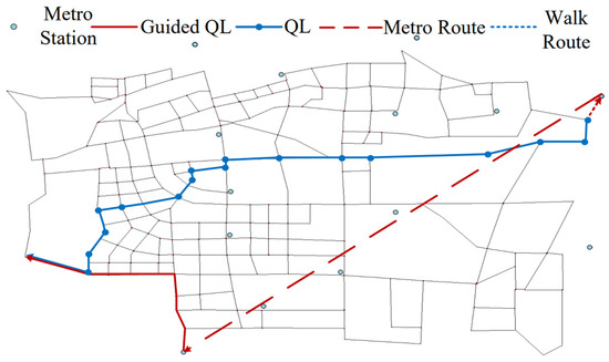
Figure 18. MT travel path.

5.2.4. TT Travel Mode

For the TT travel mode, in cases where both the passenger’s origin and destination lie outside the subway station’s attraction zone, the GQL algorithm suggests utilizing ride-hailing services for the complete trip. The algorithm has provided two different routes, as shown in Figure 19, and the one generated by the GQL algorithm has a shorter total path length, indicating a stronger exploration ability in unknown environments.

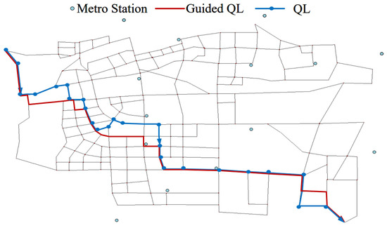
Figure 19. TT travel path.

5.3. Algorithm Comparison

The GQL algorithm is evaluated against the Sarsa and Q-learning algorithms in terms of reward value, learning duration, total path length, travel cost, and learning efficiency during the training phase for the TO travel mode. The GQL algorithm demonstrates a high level of adaptability to complex environments, enabling it to generate accurate and efficient path plans with greater precision in such settings. Furthermore, it exhibits a tendency toward greater stability upon convergence.

The GQL algorithm demonstrates accelerated convergence, resulting in a 25% reduction in training time relative to QL. At action selection, a random noise is added to the reward value for each action, as shown in Figure 20. The incorporation of random noise can facilitate a more exploratory approach to the algorithmic process, thereby enabling the intelligent system to identify novel optimization pathways within an uncharted domain. This exploratory nature assists in circumventing the pitfalls of local optimal solutions and enables a more comprehensive exploration of the state space, thereby enhancing the algorithm’s resilience and generalizability. During the initial training, the standard QL algorithm has an initial negative reward of −217,356, while the GQL algorithm has a significantly lower negative reward of −81,751. Similarly, the longest initial learning time of QL is 4642 in Figure 21, whereas the GQL algorithm has a shorter initial learning time of only 1877. Overall, the GQL algorithm demonstrates lower reward values, reduced learning time, and smoother overall fluctuations compared to the standard QL algorithm.

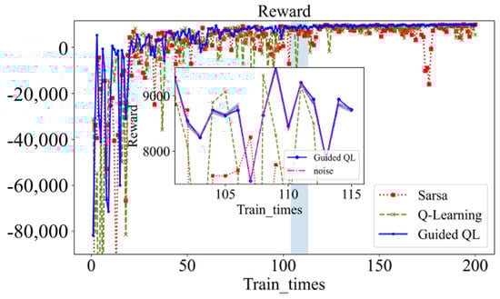
Figure 20. Comparison of reward values.

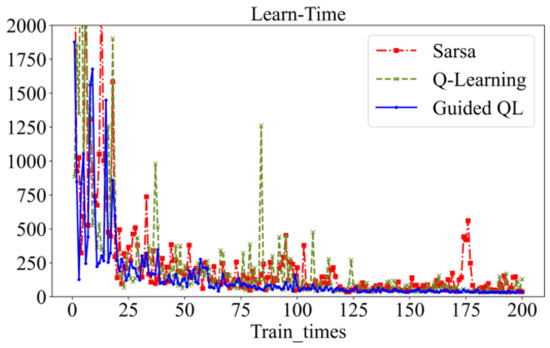
Figure 21. Comparison of Learn-Time.

Compared with the QL and Sarsa algorithms, the GQL algorithm achieves an 11% reduction in minimum travel cost and an 8% reduction in optimal path length. This means that the GQL algorithm is able to find more efficient and economical travel paths for the same travel demand. In the initial training phase, the GQL algorithm exhibits a relatively small path length and low traveling cost. However, the Q-learning and Sarsa algorithms display a slight degree of fluctuation following convergence, particularly during the mid-training period. The Q-learning algorithm exhibits a significant level of variability in average path length, travel cost, and travel time, as evidenced by the substantially greater fluctuations observed in comparison to the mean, illustrated in Figure 22. In contrast, the Sarsa algorithm exhibits a relatively stable performance across the entire training phase. The Sarsa algorithm demonstrates overall stability, although some instability is observed in the middle and late stages of training. Ultimately, the convergence values of path length, traveling cost, and traveling time are higher than those of the GQL and Q-learning algorithms. Considering the same OD pairs, the travel length, time, and cost comparison among the three algorithms are presented in Table 9.

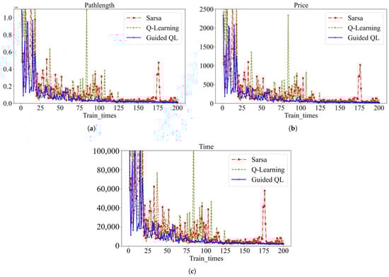
Figure 22. Comparison of path length, traveling cost, and traveling time. (a) Comparison of path length. (b) Comparison of traveling cost. (c) Comparison of traveling time.

Table 9. Comparison of travel length, time, and cost.

Mode	Q-Learning			Sarsa			GQL
	Length	Time	Cost	Length	Time	Cost	Length	Time	Cost
MM	6373	765	21.76	6138	656	20.49	5900	1380	6
TM	6687	1080	23.41	8356	1532	26.5	3052	1200	19
MT	8547	1500	26.76	5761	986	22.5	9017	1400	19
TO	9670	1800	29.34	9513	1736	28.2	9122	1560	28.08

As illustrated in Table 9, the GQL algorithm has the lowest travel cost compared to the Q-learning and Sarsa algorithms because it adds “nearest subway station” as a guiding factor to the path search algorithm. Due to the limited coverage of the subway network, the travel time and distance of the routes recommended by the GQL algorithm are slightly longer in some travel modes. However, considering the stability of subway operations, the travel time of the routes recommended by the GQL algorithm is more reliable. In terms of MT and TM travel modes, the GQL algorithm offers the most cost-effective travel solutions, with travel times that are only surpassed by the Sarsa algorithm. Consequently, passengers who prioritize convenience may opt for the Sarsa algorithm, while those seeking the most economical options may select the GQL algorithm, which surpasses the Q-learning algorithm in both cost and time efficiency. The following scenario is presented for consideration. In the case of the TO travel mode, the GQL algorithm is able to identify the solution with the shortest time and the lowest cost. Consequently, the GQL algorithm decreases the number of iterations and computational time, reduces the path length and traveling cost, and demonstrates robust adaptability to complex environments. Given that the GQL algorithm considers the metro path, the travel length and travel time are longer in some of the connecting modes compared to the Q-learning and Sarsa algorithms. However, the GQL algorithm travel time is more stable and reliable and has a greater advantage in travel cost.

The consideration of a range of potential connections affords passengers a broader selection of more cost-effective travel options, with more reliable travel times and more cost-effective travel costs. However, it should be noted that some of the connecting modal path lengths may be longer. The advantages of integrating ride-hailing services with rail transit are summarized as follows:

• More reliable travel time. With the fixed operating routes and schedules of rail transit systems, passengers can accurately estimate their travel time. The combination of ride-hailing and rail transit modes can also provide more efficient transfer services, reducing transfer time.
• Cost savings. Passengers can save costs during their journey by only paying for ride-hailing and rail transit fares, without additional expenses such as parking fees or congestion charges.
• Optimized travel routes. The integration of ride-hailing and rail transit can offer passengers more optimized travel routes, reducing travel time by avoiding congested routes and crowded areas.
• Suitable for various types of travelers. Ride-hailing services connecting with rail transit can cater to a wide range of travelers, providing diverse options for travel routes. Passengers can choose the most suitable travel path based on their individual needs and preferences.

By considering the rail transit network in addition to ride-hailing services, GQL considers the subway path, so compared with QL, the trip length and trip time are both longer, but the trip time is more stable and reliable, and the trip cost has some advantages. Overall, the integration of ride-hailing with rail transit offers a more efficient and personalized travel experience for passengers.

6. Conclusions

This paper analyzes real data through clustering analysis and road network modeling and identifies the hotspots for passenger pick-up and drop-off. Buffer zones are set around the subway stations to analyze the connection modes for ODs. This paper proposes an algorithm for short-distance travel decision-making in online ride-hailing integrated with rail transit, grounded in reinforcement learning. The GQL algorithm is utilized to construct a network topology model reflecting the real road network, determine the optimal route across different connectivity scenarios, and formulate both the Q-table initialization approach and the action selection mechanism of the GQL algorithm tailored to the specific attributes of path planning. By adding the guiding principle of reinforcing experience and including “nearest subway station” as the guiding factor in the path search algorithm, blind search is avoided, and different connection modes exhibit better path planning performance based on prior experience.

Extensive experiments carried out in SUMO simulation environments with varying scales, scenarios, and features have robustly demonstrated the viability and efficiency of the proposed approach. The convergence speed is enhanced by 25% when compared to the conventional QL algorithm. The optimal path length is decreased by 8%, and the minimal travel cost is lowered by 11%. The algorithm exhibits robust adaptability to intricate and uncertain environments, efficiently decreasing both the number of iterations and computational time. By incorporating ride-hailing services with rail transit for transportation, this method helps lower passengers’ overall travel expenses. It effectively addresses the “last mile” problem in transportation and provides users with a more convenient, intelligent, and environmentally friendly travel experience.

A limitation of this paper is that the dataset only includes GPS data from ride-hailing vehicles in Fengtai District, Beijing, China, over a continuous week. Future research could incorporate data from additional regions and longer time periods to capture travel patterns that vary by location or season.

References

- Bhellar, M.G.; Talpur, M.A.H.; Khahro, S.H.; Ali, T.H.; Javed, Y. Visualizing Travel Accessibility in a Congested City Center: A GIS-Based Isochrone Model and Trip Rate Analysis Considering Sustainable Transportation Solutions. Sustainability 2023, 15, 16499. [Google Scholar] [CrossRef]
- Liu, Z.; Yu, B.; Zhang, L.; Sun, Y. Resilience enhancement of multi-modal public transportation system via electric bus network redesign. Transp. Res. Part E Logist. Transp. Rev. 2025, 193, 103810. [Google Scholar] [CrossRef]
- Wu, Q.; Li, Y.; Dan, P. Optimization of urban rail transit station spacing for minimizing passenger travel time. J. Rail Transp. Plan. Manag. 2022, 22, 100317. [Google Scholar] [CrossRef]
- Liu, X.H.; Shao, X.; Li, Y. Eco-friendly integration of shared autonomous mobility on demand and public transit based on multi-source data. Inf. Fusion 2024, 115, 102771. [Google Scholar] [CrossRef]
- Ni, Y.; Zhuo, Q.; Li, N.; Yu, K.; He, M.; Gao, X. Characteristics and Optimization Strategies of A* Algorithm and Ant Colony Optimization in Global Path Planning Algorithm. Int. J. Pattern Recognit. Artif. Intell. 2023, 37, 2351006. [Google Scholar] [CrossRef]
- Ma, C.X.; Zhao, M.X.; Liu, Y. Vehicle navigation path optimization based on complex networks. Phys. A—Stat. Mech. Its Appl. 2025, 665, 130509. [Google Scholar] [CrossRef]
- Liu, B.; Jin, S.K.; Li, Y.Z.; Wang, Z.; Zhao, D.L.; Ge, W.J. An Asynchronous Genetic Algorithm for Multi-agent Path Planning Inspired by Biomimicry. J. Bionic Eng. 2025, 22, 851–865. [Google Scholar] [CrossRef]
- Xu, H.; Niu, Z.J.; Jiang, B.; Zhang, Y.H.; Chen, S.J.; Li, Z.Q.; Gao, M.K.; Zhu, M.K. ERRT-GA: Expert Genetic Algorithm with Rapidly Exploring Random Tree Initialization for Multi-UAV Path Planning. Drones 2024, 8, 367. [Google Scholar] [CrossRef]
- Sheng, C.Y.; An, H.; Nie, J.; Wang, H.X.; Lu, X. Improved M-DQN With ε-UCB Action Selection Policy and Multi-Goal Fusion Reward Function for Mobile Robot Path Planning. IEEE Trans. Veh. Technol. 2025, 74, 5358–5370. [Google Scholar]
- Li, Z.; Han, S.; Chen, Y.; Ning, X. A Path Planning Algorithm for Mobile Robots Based on Angle Searching and Deep Q-Network. Acta Armamentarii 2025, 46, 30–44. [Google Scholar]
- Lei, K.; Guo, P.; Wang, Q.; Zhao, W.; Tang, L. End-to-end deep reinforcement learning framework for multi-depot vehicle routing problem. Appl. Res. Comput. 2022, 39, 3013–3019. [Google Scholar]
- Zhou, Q.; Lian, Y.; Wu, J.Y.; Zhu, M.Y.; Wang, H.Y.; Cao, J.L. An optimized Q-Learning algorithm for mobile robot local path planning. Knowl.-Based Syst. 2024, 286, 111400. [Google Scholar] [CrossRef]
- Wang, X.; Ji, J.; Liu, Y.; He, Q. Path Planning of Unmanned Delivery Vehicle Based on Improved Q-learning Algorithm. J. Syst. Simul. 2024, 36, 1211–1221. [Google Scholar]
- Zhang, T.; Cheng, J.; Zou, Y.B. Multimodal transportation routing optimization based on multi-objective Q-learning under time uncertainty. Complex Intell. Syst. 2024, 10, 3133–3152. [Google Scholar] [CrossRef]
- Zhong, Y.; Wang, Y.H. Cross-regional path planning based on improved Q-learning with dynamic exploration factor and heuristic reward value. Expert Syst. Appl. 2025, 260, 125388. [Google Scholar] [CrossRef]
- Wei, J.; Long, K.; Gu, J.; Ju, Q.; Zhu, P. Optimizing Bus Line Based on Metro-Bus Integration. Sustainability 2020, 12, 1493. [Google Scholar] [CrossRef]
- Song, Y.; Wang, Z.; Wang, R. Research on Travel Paths Based on Car-Hailing Services Connecting with Rail Transit. In Proceedings of the 2023 IEEE 26th International Conference on Intelligent Transportation Systems (ITSC), Bilbao, Spain, 24–28 September 2023; pp. 1686–1691. [Google Scholar]
- Peng, Z.; Sun, S.; Tong, L.; Fan, Q.; Wang, L.; Liu, D. Optimization of offshore wind farm inspection paths based on K-means-GA. PLoS ONE 2024, 19, e0303533. [Google Scholar] [CrossRef]
- Su, H.T.; Li, M.H.; Zhong, X.F.; Zhang, K.; Wang, J.K. Estimating Public Transportation Accessibility in Metropolitan Areas: A Case Study and Comparative Analysis. Sustainability 2023, 15, 12873. [Google Scholar] [CrossRef]
- Jin, R.Y.; Xu, P.; Gu, J.F.; Xiao, T.; Li, C.H.; Wang, H.X. Review of optimization control methods for HVAC systems in Demand Response (DR): Transition from model-driven to model-free approaches and challenges. Build. Environ. 2025, 280, 113045. [Google Scholar] [CrossRef]
- Haliem, M.; Mani, G.; Aggarwal, V.; Bhargava, B. A Distributed Model-Free Ride-Sharing Approach for Joint Matching, Pricing, and Dispatching Using Deep Reinforcement Learning. IEEE Trans. Intell. Transp. Syst. 2021, 22, 7931–7942. [Google Scholar] [CrossRef]
- Zhang, W.Y.; Xia, D.W.; Chang, G.Y.; Hu, Y.; Huo, Y.J.; Feng, F.J.; Li, Y.T.; Li, H.Q. APFD: An effective approach to taxi route recommendation with mobile trajectory big data. Front. Inf. Technol. Electron. Eng. 2022, 23, 1494–1510. [Google Scholar] [CrossRef]
- Wang, Z.; Yang, J.; Zhang, Q.; Wang, L. Risk-Aware Travel Path Planning Algorithm Based on Reinforcement Learning during COVID-19. Sustainability 2022, 14, 13364. [Google Scholar] [CrossRef]
- Yan, G.; Ning, L. Path planning of UAV using guided enhancement Q-learning algorithm. Acta Aeronaut. Astronaut. Sin. 2021, 42, 325109. [Google Scholar]
Disclaimer/Publisher’s Note: The statements, opinions and data contained in all publications are solely those of the individual author(s) and contributor(s) and not of MDPI and/or the editor(s). MDPI and/or the editor(s) disclaim responsibility for any injury to people or property resulting from any ideas, methods, instructions or products referred to in the content. |
© 2025 by the authors. Licensee MDPI, Basel, Switzerland. This article is an open access article distributed under the terms and conditions of the Creative Commons Attribution (CC BY) license (https://creativecommons.org/licenses/by/4.0/).