Abstract
Wheel slipping during trajectory tracking presents significant challenges for wheeled mobile robots (WMRs), degrading accuracy and stability on low-friction or dynamic terrain. Effective control requires addressing unknown slipping parameters while balancing tracking precision and energy efficiency. To address this challenge, a control framework integrating a sliding mode observer (SMO), an improved particle swarm optimization (PSO) algorithm, and a linear quadratic regulator (LQR) is proposed. First, a dynamic model incorporating longitudinal slipping is established. Second, an SMO is designed to estimate the slipping ratio in real-time, with chattering suppressed using a low-pass filter. Finally, an improved PSO algorithm featuring a nonlinear cosine-decreasing inertia weight strategy optimizes the LQR weighting matrices (Q/R) online to both minimize tracking errors and control energy consumption. Simulations including both circular and sine wave trajectories demonstrate that the SMO achieves rapid and accurate slipping ratio estimation, while the PSO-optimized LQR significantly enhances tracking accuracy, achieves smoother control inputs, and maintains stability under varying slipping conditions.
1. Introduction
Wheeled Mobile Robots (WMRs) have emerged as a transformative technology in modern automation, driving innovation in advanced manufacturing, logistics, agriculture, and service sectors. Their ability to navigate dynamic environments flexibly and efficiently makes them indispensable in scenarios ranging from precision material handling to autonomous field operations [1,2,3]. However, their practical deployment is constrained by two critical challenges: inherent nonholonomic motion constraints, which complicate control design, and unavoidable wheel slipping—caused by low-friction surfaces, abrupt acceleration, or uneven terrain—which introduces nonlinearity and uncertainty, degrading tracking accuracy and threatening stability.
Existing trajectory tracking methods for WMRs, such as sliding mode control [4,5,6], backstepping control [7,8,9], fuzzy logic control [10,11,12], adaptive control [13,14,15], neural network-based control [16,17,18], active disturbance rejection control [19,20,21], and pure pursuit control [22,23], have achieved significant progress but often rely on idealized assumptions of zero wheel slipping. In reality, slipping disrupts the kinematic relationship between wheel motion and robot pose, leading to accumulated errors and potential instability. This gap between theory and practice underscores the need for robust control strategies that explicitly address slipping.
Recent efforts to mitigate slipping effects have followed two main methods. One approach treats slipping as a lumped disturbance, using observers to compensate for its impact. For example, Kang et al. [24] employed a generalized extended state observer (GESO) to estimate lumped disturbances, including unknown slipping and sliding effects, subsequently proposing a GESO-based robust tracking controller. Li et al. [25] proposed a novel fixed-time control scheme. This method constructs a fixed-time velocity control law using intermediate variables to avoid singularity issues and develops a fast fixed-time disturbance observer to estimate slipping and external disturbances. Experiments have verified that it can achieve high-precision tracking within a preset time. Chen et al. [26] obtained the virtual velocity control law via a desired disturbance observer, later formulating a robust tracking control method aligned with the actual system’s trajectory goal. Nie et al. [27] proposed a low-complexity safety control method. This method overcomes the limitations of traditional model control point selection by introducing a novel linearization model combined with virtual points and directly constrains the tracking error using a preset performance function. It achieves the goal of strictly limiting the robot trajectory tracking error within a preset safety range without the need to obtain or estimate complex slipping parameters. In reference [28], autoregressive wavelet neural networks were used to approximate model uncertainties and slipping limitations. This enabled the development of a controller that can track a trajectory in an adaptive manner and avoid obstacles. Ryu et al. [29] designed a robust controller treating wheel slipping as lumped disturbance, validating its effectiveness via simulation and experiment. FEI et al. [30] presented a nonlinear extended state observer (NESO) leveraging fuzzy neural networks to estimate system states and total disturbances, thereby enabling active compensation for unmodeled dynamics. In addition, data-driven control strategies, such as the γ-DDPC framework proposed by Breschi et al. [31], provide a new way of thinking about wheeled robot slip as system uncertainty by dealing with system uncertainty and noise through regularization techniques. The studies mentioned above all treat slipping as a black-box disturbance, failing to leverage the internal parameter information of slipping. Controller parameters are not dynamically adjusted based on the slipping magnitude, which may restrict performance under varying slipping conditions.
The second path involves slipping parameter estimation. Wang et al. [32] established a mathematical model incorporating both skidding and sliding dynamics. Cui et al. [33] proposed an adaptive tracking control scheme for wheeled mobile robots with unknown longitudinal and lateral slipping by integrating a sliding mode observer for real-time slipping parameter estimation and a backstepping controller, guaranteeing global stability via the Lyapunov theory and demonstrating robust performance under large initial errors. Song et al. [34] proposed a nonlinear sliding mode observer to estimate the slipping parameters of unmanned wheeled vehicles with high accuracy, verifying its effectiveness using dedicated linear and 2D test benches. However, these methods [32,33,34] typically estimate the slipping ratio as a system parameter but lack adaptation of the controller parameters based on the estimated slipping conditions. Consequently, the controller struggles to maintain optimal performance across varying slipping conditions.
Ni et al. [35] designed an improved LQR controller, integrating feedforward control and an adaptive gain strategy for real-time QR matrix adjustment based on tracking error. The above literature is able to adjust the LQR controller parameters in real time according to the error, but not according to the difference in the system slipping ratio.
In summary, existing methods have not yet solved the problem of real-time weight optimization updates under different slipping parameters. In this paper, we estimate the slipping ratio parameters in real time and use the improved PSO algorithm to combine with the LQR controller to adjust the parameter sizes of the controller to dynamically adapt the controller to varying slipping conditions and operational scenarios. The main contributions of this article are as follows:
- (1)
- To address the model mismatch problem introduced by unknown slipping parameters, a kinematic model incorporating longitudinal slipping dynamics is derived to characterize the system behavior, a sliding mode observer is used to observe the slipping parameter, and a first-order low-pass filter is used to reduce the chattering phenomenon.
- (2)
- To reduce reliance on empirical selection of LQR weights, a PSO algorithm with nonlinear inertia weights is proposed to optimize the Q/R matrix in real time to improve the tracking performance of the controller.
- (3)
- A closed-loop framework integrating slipping estimation and optimization control is constructed, significantly enhancing the tracking accuracy, control smoothness, and robust stability of WMRs with unknown slipping condition.
2. Kinematic Modeling with Slipping
There are many types of wheeled mobile robots, among which two-wheeled differential drive robots are favored due to their advantages of exhibiting a simple structure and a flexible control system. Figure 1 shows a classic kinematic model of a two-wheel differentially driven wheeled mobile robot. The structure includes a frame of coordinates , centered at the coordinate origin, and a frame of move coordinates , with the geometric center O as the origin ω, denotes the angular velocity of the mobile robot, which is rotating around the origin O of the coordinate system . Instead of a steering mechanism, the robot achieves turning by adjusting the speed difference between the two wheels to realize the sliding of the robot body, then completing the steering action of different radii. To simplify the model analysis, it is assumed that the body is perfectly symmetrical and that the center of mass of the robot and the center of its shape are not offset from one point. In this study, we focused on the longitudinal slipping phenomenon. In the ideal case of a wheel without slipping, its kinematics can be expressed as
where r denotes the wheel’s rolling radius, the linear and angular velocities of the left wheel are denoted by and , and the linear and angular velocities of the right wheel are denoted by and .
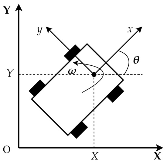
Figure 1.
Kinematic modeling of WMR with differential drive.
As Figure 1 shows, the forward velocity v and the steering angular velocity ω can be characterized by the following equation:
where b denotes the wheelbase.
To describe the phenomenon of longitudinal slipping more accurately, the concept of a longitudinal wheel slipping ratio is introduced. The introduction of the longitudinal wheel slipping ratio means that the linear velocities of the left and right wheels become
where is the left wheel slipping ratio, and is the right wheeled slipping ratio.
In coordinate system , without wheel slipping, the position and attitude of WMR can be described as follows:
With the introduction of the longitudinal slipping ratio in the standard model, the model with longitudinal slipping included in the coordinate system can be defined as described below:
As shown in Figure 1, there is a transformation relationship between coordinate system and coordinate system , and the transformation equation between them is shown below:
Therefore, the following equation can be applied in order to represent the WMR’s kinematic model within the global reference system , considering the longitudinal slipping case:
3. Mobile Robot Trajectory Tracking Model
During the trajectory tracking process, the mobile robot must determine the error between its actual pose and the desired pose in real time in order to promptly adjust its control strategy. When tracking a given reference trajectory, the trajectory tracking diagram can be simplified to that shown in Figure 2. The variables and denote the true and desired positions of the mobile robot, respectively, and the relationship between these positions is given by the following kinematic equations:
where denotes the transverse error, denotes the longitudinal error, and denotes the directional error.
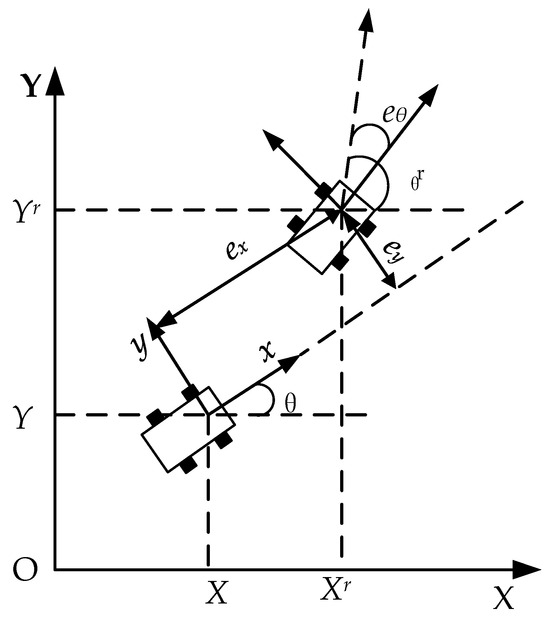
Figure 2.
Schematic diagram of trajectory tracking of a wheeled mobile robot.
Applying the derivative to Equation (8) yields
where represents the angular velocity control input, v denotes the linear velocity control input, is the reference angular velocity, and denotes the reference linear velocity.
This is obtained by linearizing the system equation at the tracking trajectory.
4. Slipping Estimation Using Sliding Mode Observer
4.1. Sliding Mode Observer Design
The measurement of the longitudinal slipping ratio of the wheel is challenging due to the complexity of direct measurement and the presence of noise in the measurement data. The sliding mode observer exhibits strong robustness to model uncertainty and noise. Therefore, a sliding mode observer is employed to estimate the longitudinal slipping ratio of each wheel. Here, , , and are used to denote the estimation of the position and angle of the WMR. represents the estimated linear velocity of the WMR, and represents its estimated angular velocity.
The above analysis leads to the design of a sliding mode observer with respect to position, angle, and linear velocities.
in the equation, , , , , and represent the sliding mode gain.
Calculate the wheel speed using the wheel speed formula:
where b is the wheelbase, the estimated linear velocities for the left and right wheels are and , respectively.
Therefore, the estimated slipping ratio of the wheel is calculated by the following equation:
where r is the wheel radius, indicates an estimate of the left-hand wheel slipping ratio, and indicates an estimate of the right-hand wheel slipping ratio. and are the commanded angular velocities of wheels, and denotes the threshold to avoid dividing by zero.
Additionally, a low-pass filter (LPF) is employed to mitigate the chattering phenomenon inherent in the sliding mode observer (SMO). It is designed as shown in Figure 3, and the relationship between input u and output y of LPF is given as
where , and , , are the filter parameters, and u is the input.
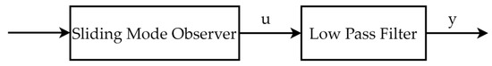
Figure 3.
Filtering process for slipping ratio estimation.
The relationship between the cutoff frequency and filter parameters is as follows:
With a cut-off frequency of , the LPF effectively attenuates high-frequency oscillations while preserving the essential dynamic characteristics of the slip ratio signal. Furthermore, owing to its structural simplicity and computational efficiency, the filter is well-suited for real-time implementation in embedded systems.
4.2. Proof of Sliding Mode Observer
In this section, the stability of the sliding mode observer is proven using the Lyapunov theory.
The switching function of the SMO is defined by the following equation:
As noted in reference [36], a sliding mode observer achieves stability only if 1. the error state converges to the sliding mode surface from any initial error in finite time; 2. the system exhibits stability within a neighborhood of this surface. Select the appropriate sliding mode gain so that , i = 1, 2, 3.
Define the positive definite Lyapunov function:
Since the slipping ratio is physically bounded, and .
It is evident that there is an inherent upper limit that exists between the actual velocity difference and the estimated velocity difference.
where and are constants greater than zero.
The estimated speed is usually constrained by the control inputs:
where is a constant greater than zero.
Angular observation error is bounded in system operation:
where M is a constant greater than zero.
Furthermore, the trigonometric functions satisfy Lipschitz continuity:
Thus,
identically obtained.
Define the upper bound:
Taking the time derivative of Equation (17) yields
From Equations (22)–(24), we derive
Since the sign function satisfies .
Thus,
Select sliding mode gain , , and so that the following satisfies the requirement.
Consequently, we have
As can be seen from the above analysis, when sliding mode gains of , , and satisfy Equation (28), the observation error of the sliding mode observer converges to zero within a finite time.
5. LQR Control Design with PSO-Based Optimization
5.1. Linearization of System Equations
Applying the linear quadratic regulator (LQR) to nonlinear systems offers significant advantages in solving control problems. However, wheeled mobile robot systems are nonlinear. Therefore, to apply the LQR controller, the system equations need to be linearized near the operating point. The linearized system matrix is as follows:
The cost function [37] is given by the following equation:
where , , , represent the weight coefficient of , , . , and denote the weight coefficients of the control inputs v and w.
The matrix K is given by the following equation:
The P matrix is a constant matrix whose exact value can be derived by solving the Riccati equation, whose mathematical expression is shown below:
Therefore, the control law is applied to the system, which can minimize the system’s performance index , and , are the feedback coefficients of LQR control.
As shown above, the system’s optimal control performance is primarily affected by the weight matrices Q and R. However, there is no fixed pattern for the selection of these two matrices, and it is usually chosen empirically by the designer. Not only is it difficult to ensure that the final output of the optimal feedback control coefficients will lead to a truly optimal system, but the whole process is time-consuming. The adverse effect of subjectivity that arises from relying on experience to determine the optimality of the system can be mitigated by using the PSO algorithm to optimize the weight matrices.
5.2. Enhanced PSO with Nonlinear Inertia Weight Strategy
Particle swarm optimization (PSO) was proposed in 1995 [38], and the idea behind its design is inspired by the cooperative behavior of groups of organisms, such as birds and fish. In the algorithm, each candidate solution is treated as a particle, which dynamically adjusts its flight direction and velocity in the solution space by tracking its individual optimal and population optimal positions. This process gradually approaches the optimal solution. The following equations are utilized in order to effect changes in the velocity and position of each individual particle:
where is the non-negative inertia weight; and are the best past positions of the individual and the population; is the velocity of the ith particle; and represent the individual learning factor and group learning coefficients, respectively; and denote two random numbers uniformly distributed in the range [0, 1], which serve to introduce randomness and make the search process randomly exploratory; denotes the current position of the i-th particle.
The inertia weight exerts significant impacts on the global optimization performance, and compared to fixed inertia weights, the linear decreasing inertia weight strategy [39] improves the performance, i.e., the inertia weight decreases linearly, leading to faster fitness function convergence compared to that of fixed weights.
The decreasing inertia weight factor of the PSO algorithm optimized using the strategy of linear decreasing inertia weight is as follows:
the inertia weight coefficient for the Tth iteration is represented as , the maximum value is , and denotes the minimum value of the inertia weights. T denotes the number of iterations currently in progress. It is important to note that the maximum number of iterations that can be performed is denoted by N.
Although the linear decreasing inertia weight strategy outperforms that of fixed weights, it still exhibits limitations; the global search duration is short in the early iterations, the local search ability is weak, and it can easily miss the global optimum. Therefore, this paper proposes a nonlinear decreasing weight update strategy:
the inertia weight coefficient for the Tth iteration is represented as , the maximum value is , denotes the minimum value of the inertia weights, and T denotes the number of iterations currently in progress. It is important to note that the maximum number of iterations that can be performed is denoted by N.
With this weight adjustment strategy, the inertia weight value at the beginning of the iteration is large and decreases slowly, enhancing exploration of the solution space, and the inertia weights decrease rapidly as the number of iterations approaches the maximum number of iterations, enhancing focusing on the optimal solution and preventing convergence to local optimality. The comparison between the linear decreasing inertia weighting strategy and the cosine decreasing inertia weighting strategy is shown in Figure 4.
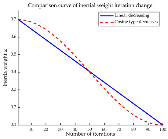
Figure 4.
Comparison curves for iterative changes in weights.
The fitness function employs a weighted performance index to satisfy both the tracking performance and energy efficiency, and the fitness function is as follows:
where ISE is the integrated squared error, E is the energy consumption of the control input, and is the terminal position error. Each component is defined as
where denotes the transverse error, the longitudinal error is represented by and denotes the angular error. T denotes the simulation time
where denotes control input.
where and denote the position of the wheeled mobile robot at the final moment, and and indicate the expected position at the final moment.
The flow diagram of the algorithm using the cosine weight update strategy is shown in Figure 5.
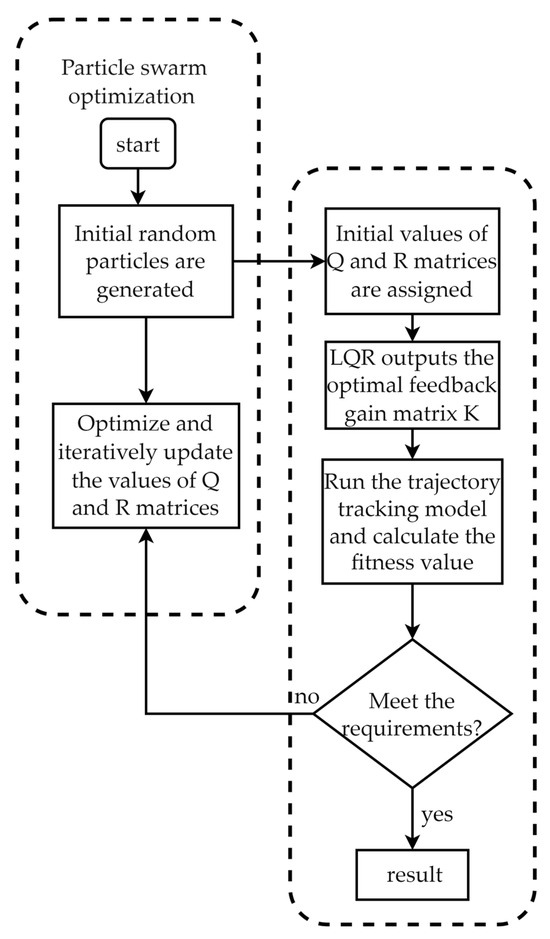
Figure 5.
Flowchart of PSO algorithm optimization.
6. Simulation Results
In this section, we will apply the formulas derived in prior sections to simulate the WMR with longitudinal slipping. To rigorously evaluate the tracking performance of the controller under varying operating conditions, two reference trajectories are selected for simulation: a circular trajectory and a sine wave trajectory. The relevant parameters of wheeled mobile robots are shown in Table 1. The five observation gains of the sliding mode observer are selected as shown in Table 2. The robot’s position is directly measurable via sensors. If the population size is too small, it tends to fall into local optimization, and if the population size is too large, the growth is no longer significant; the maximum number of iterations, as the termination condition of the optimization, takes too long to optimize if it is too large, and optimization is terminated before reaching the optimal result if it is too small. A good balance between the algorithm’s solution speed and the quality of the optimal solution can be achieved by using the following particle swarm optimization (PSO) parameter configurations. The parameter configurations of the improved particle swarm optimization algorithm are shown in Table 3. We analyzed the computational load of the PSO algorithm. The optimization process was performed using MATLAB 2024a on a desktop platform (Intel i7-12700 K DELL, Xiamen, China), with each run taking approximately 120 s.

Table 1.
Parameters of WMR.
Table 2.
Parameters of SMO.
Table 3.
Parameters of PSO.
To compare the effectiveness of the three weighted updating methods, we choose a circular reference trajectory for simulation, whose specific parameters are given in Section 6.1, and the fitness convergence curve is shown in Figure 6.
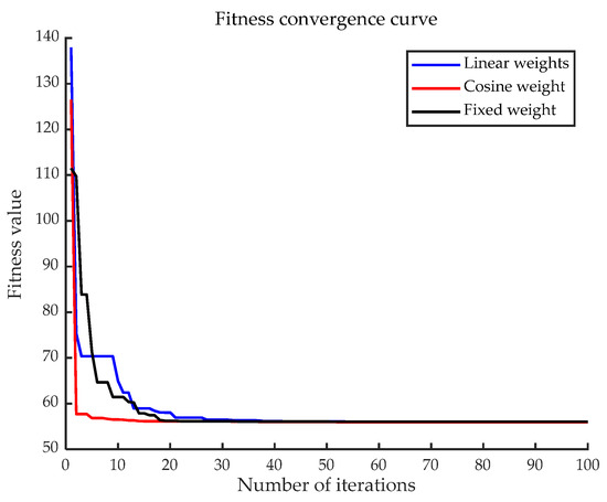
Figure 6.
Fitness convergence curve.
As shown in the results, the cosine weights updating method proposed in this paper exhibits the fastest decreasing adaptation and the smallest final adaptation. The PSO-optimized LQR algorithm proposed in this paper displays a large searchable space and a high probability of finding the optimal solution in the early iteration period due to the slow reduction of inertia weights and avoids falling into a local optimum in the later stage due to the fast decrease in inertia weights, finding better approximate solutions.
6.1. Circular Trajectory Simulation
The equation for a given circular reference trajectory is
where t denotes the simulation time, 0 < t < 50 s.
The linear velocity of the WMR is expected to be ; the expected angular velocity is . The parameters of the Q, R matrix optimized by the PSO are as follows: Q = diag [11.760, 29.763, 12.219], R = diag [0.010, 0.010], and the initial position and orientation of the WMR are set as . The initial desired pose is given by the trajectory equation . The verification of tracking performance in the slipping case will be performed according to the following parameters, i.e., the abrupt change of and parameters is simulated, and it is assumed that , and at t = 15 s. For comparison, unoptimized Q and R matrices are selected, i.e., Q = diag [10, 10, 8]; R = diag [1, 1]. The tracking results are shown in Figure 7, Figure 8, Figure 9 and Figure 10. Two performance indicators were selected: maximum deviation and convergence time. The maximum deviation value was deviation. The convergence time is the time required for the error to enter and remain within the steady-state band (5%). The two performance indicators of the circular reference trajectory are shown in Table 4.
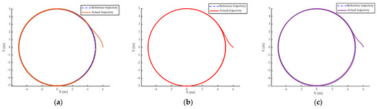
Figure 7.
Circular trajectory tracking results: (a) conventional LQR (fixed Q, R); (b) PSO−optimized LQR; (c) reference [33] method.
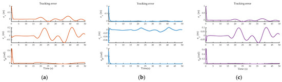
Figure 8.
Circular trajectory tracking error: (a) conventional LQR (fixed Q, R); (b) PSO−optimized LQR; (c) reference [33] method.
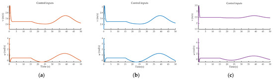
Figure 9.
Circular trajectory control inputs: (a) conventional LQR (fixed Q, R); (b) PSO−optimized LQR; (c) reference [33] method.
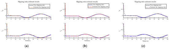
Figure 10.
Circular trajectory slipping ratio estimation: (a) conventional LQR (fixedQ R); (b) PSO−optimized LQR; (c) reference [33] method.
Table 4.
Circular reference trajectory performance indicators.
As illustrated in Figure 7 and Figure 8, a comparison of the steady-state error between the optimized model and the baseline model demonstrates a significant reduction in error magnitude following optimization. Figure 8 further reveals that the conventional LQR controller experiences substantial tracking deviations once wheel slipping occurs. Conversely, Figure 10 indicates that the SMO converges to the true slipping ratio within 3 s, thereby delivering precise parameter updates to the PSO-LQR controller. This integrated “estimation-optimization” closed-loop architecture sustains system stability under conditions of unknown slipping and effectively mitigates the tracking divergence problem inherent in traditional LQR controllers when confronted with model uncertainties.
A quantitative analysis of the performance indicators in Table 4 further supports these observations. The PSO-optimized LQR achieves a maximum deviation of only 0.09 m, significantly lower than the 0.35 m of the conventional LQR and also superior to the 0.15 m of the reference [33] method. Regarding convergence time, the PSO-LQR (1.19 s) shows a slight improvement over the conventional LQR (1.23 s), although it is slightly slower than the reference [33] method (0.85 s). This indicates that while the PSO-LQR may not be the fastest in terms of initial convergence, it offers a superior balance by achieving significantly higher steady-state accuracy, which is often more critical for precise trajectory tracking.
6.2. Sine Wave Trajectory Simulation
The sine wave reference trajectory is defined as
where t denotes the simulation time, 0 < t < 50 s. The original coordinates of the wheeled mobile robot are defined as follows: . The initial desired pose is assigned a value of . The verification of tracking performance in the slipping case will be performed according to the following parameters, i.e., the abrupt change of parameter is simulated, and it is assumed that becomes 0.1 and becomes 0.15 at t = 10 s. The parameters of the Q and R matrix optimized by the PSO algorithm are as follows: Q = diag [8.916, 19.920, 14.607], and R = diag [0.026, 0.050]. At the same time, SMO can accurately track changes in slipping parameters. Unoptimized Q and R matrices are selected, i.e., Q = diag [10, 10, 5], and R = diag [8, 8]. The simulation results are shown below in Figure 11, Figure 12, Figure 13 and Figure 14. The two performance indicators of the sine wave reference trajectory are shown in Table 5.
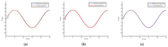
Figure 11.
Sine wave trajectory tracking results: (a) conventional LQR (fixed Q, R); (b) PSO−optimized LQR; (c) reference [33] method.
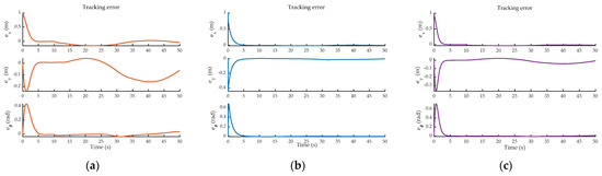
Figure 12.
Sine wave trajectory tracking error: (a) conventional LQR (fixed Q, R); (b) PSO−optimized LQR; (c) reference [33] method.
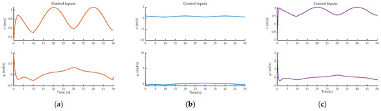
Figure 13.
Sine wave trajectory tracking control inputs: (a) conventional LQR (fixedQ R); (b) PSO−optimized LQR; (c) reference [33] method.
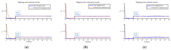
Figure 14.
Sine wave trajectory tracking slipping ratio estimation: (a) conventional LQR (fixedQ R); (b) PSO−optimized LQR; (c) reference [33] method.
Table 5.
Sine wave reference trajectory performance indicators.
The sine wave reference trajectory exhibits significant periodic curvature fluctuations, which poses a serious challenge to the trajectory tracking control due to its stringent dynamic requirements. As shown in Figure 11a and Figure 12a, the LQR controller with unoptimized parameters exhibits significant limitations when tracking such complex paths. Large tracking errors are observed, particularly in intervals where curvature is maximal.
The performance metrics in Table 5 provide a clear quantitative comparison. The maximum deviation for the conventional LQR is 0.15 m, which is reduced to 0.06 m by the PSO-LQR, matching the performance of the reference [33] method. For convergence time, the PSO-LQR (2.77 s) shows a notable improvement over that in the conventional LQR (3.21 s), although it remains slightly slower than in the reference [33] method (2.26 s). These results demonstrate that the proposed PSO-LQR controller effectively handles the challenging sine wave trajectory, achieving high tracking accuracy and improved convergence compared to those of the conventional approach, while generating smoother control inputs, as seen in Figure 13b.
In contrast, the control input transitions smoothly between acceleration and deceleration phases, directly enhancing system durability. These improvements confirm the controller’s effectiveness in complex navigation scenarios with continuously changing curvature.
7. Conclusions
In this study, the key challenge of the trajectory tracking control of wheeled mobile robots (WMRs) with wheel slipping is addressed. To improve tracking accuracy and robustness, an integrated control framework is proposed, combining three key components: First, a dynamic model incorporating longitudinal slipping parameters is developed. Second, a sliding mode observer (SMO) with an LPF is designed. The SMO provides a fast and accurate estimation of the slipping ratio, while the low-pass filter effectively suppresses chattering of the observation. Finally, the LQR controller parameters are optimized by PSO. The improved PSO algorithm with nonlinear cosine decreasing inertia weights optimizes the Q and R matrices in the LQR cost function to minimize the tracking error and control energy consumption. This is validated by extensive simulations of circular and sine wave trajectories. Compared to a manually adjusted LQR, the PSO-LQR controller significantly reduces steady-state tracking errors and produces smoother control inputs. Smooth control inputs extend the service life of control motors in real-world operation. The composite framework maintains stability under complex slipping conditions, even during high curvature maneuvers. However, this study still exhibits some limitations. First, the dynamic model assumes that the robot’s mass is symmetrical and that there is no lateral slip, which may differ from certain real-world scenarios. Second, the simulation was conducted in an ideal environment and did not consider actual factors such as sensor noise and communication delays. Future work will focus on verifying this algorithm using a physical experimental platform and further studying the incorporation of lateral slip and more complex dynamic models into the control framework.
Author Contributions
Conceptualization, P.T. and M.C.; methodology, P.T. and M.C.; software, P.T. and S.C.; validation, P.T., M.C. and L.Z.; formal analysis, P.T., S.C., R.W. and L.Z.; data curation, S.C. and R.W.; writing—original draft preparation, P.T.; writing—review and editing, M.C.; supervision, M.C.; project administration, M.C. and W.L.; funding acquisition, M.C. and W.L. All authors have read and agreed to the published version of the manuscript.
Funding
This work was supported in part by the Foundation of Henan Province Education Department of China (No. 24A413007) and by the National Natural Science Foundation Cultivation Project of Nanyang Normal University of China (No. 2024PY012, 2024PY011).
Data Availability Statement
The original contributions presented in this study are included in the article. Further inquiries can be directed to the corresponding author.
Conflicts of Interest
The authors declare no conflicts of interest.
References
- Chohan, J.S.; Bawa, G.; Hussain, A.; Al-Nafei, A.A.M.; Reddy, M.U.P.; Gehlot, A. Robotics and its control systems: Innovation overview and future challenges. In Proceedings of the 2024 11th International Conference on Computing for Sustainable Global Development (INDIACom), New Delhi, India, 28 February–1 March 2024; pp. 524–528. [Google Scholar] [CrossRef]
- Zhang, X.; Fang, Y.; Sun, N. Visual servoing of mobile robots for posture stabilization: From theory to experiments. IEEE Trans. Ind. Electron. 2017, 64, 390–400. [Google Scholar] [CrossRef]
- Cui, M.; Liu, H.; Liu, W.; Qin, Y. An adaptive unscented Kalman filter-based controller for simultaneous obstacle avoidance and tracking of wheeled mobile robots with unknown slipping parameters. J. Intell. Robot. Syst. 2018, 92, 489–504. [Google Scholar] [CrossRef]
- Park, B.S.; Yoo, S.J.; Park, J.B.; Choi, Y.H. Adaptive neural sliding mode control of nonholonomic wheeled mobile ro-bots with model uncertainty. IEEE Trans. Control Syst. Technol. 2009, 17, 207–214. [Google Scholar] [CrossRef]
- Zheng, W.; Zheng, J.; Shao, K.; Zhao, H.; Man, Z.; Sun, Z. Adaptive fuzzy sliding mode control of ucertain nnholonomic weeled mbile rbot with eternal dsturbance and atuator sturation. Inf. Sci. 2024, 663, 120303. [Google Scholar] [CrossRef]
- Chen, Y.H. Nonlinear Adaptive fuzzy hybrid sliding mode control design for trajectory tracking of autonomous mobile robots. Mathematics 2025, 13, 1329. [Google Scholar] [CrossRef]
- Chwa, D. Tracking control of differential-drive wheeled mobile robots using a backstepping-like feedback linearization. IEEE Trans. Syst. Man Cybern. A 2010, 40, 1285–1295. [Google Scholar] [CrossRef]
- Qiang, L.; Tang, H.H.; Ahmad, N.S. Improving Trajectory tracking of differential wheeled mobile robots with enhanced GWO-Optimized Back-Stepping and FOPID controllers. IEEE Access 2025, 13, 48872–48887. [Google Scholar] [CrossRef]
- Zhu, C.; Li, B.; Zhao, C.; Wang, Y. Trajectory tracking control of Car-like mobile robots based on extended state observer and backstepping control. Electronics 2024, 13, 1563. [Google Scholar] [CrossRef]
- Miranda-Colorado, R.; Cazarez-Castro, N.R. Observer-Based fuzzy trajectory-tracking controller for wheeled mobile robots with kinematic disturbances. Eng. Appl. Artif. Intell. 2024, 133, 108279. [Google Scholar] [CrossRef]
- Ding, W.; Zhang, J.-X.; Shi, P. Adaptive fuzzy control of wheeled mobile robots with prescribed trajectory tracking performance. IEEE Trans. Fuzzy Syst. 2024, 32, 4510–4521. [Google Scholar] [CrossRef]
- Alshorman, A.M.; Alshorman, O.; Irfan, M.; Glowacz, A.; Muhammad, F.; Caesarendra, W. Fuzzy-Based Fault-Tolerant control for omnidirectional mobile robot. Machines 2020, 8, 55. [Google Scholar] [CrossRef]
- Ranjbarsahraei, B.; Roopaei, M.; Khosravi, S. Adaptive fuzzy formation control for a swarm of nonholonomic differentially driven vehicles. Nonlinear Dyn. 2012, 64, 2747–2757. [Google Scholar] [CrossRef]
- Li, G.; Guo, Y.; Chi, Q.; Wang, S.; Fan, Y. Adaptive finite-Time trajectory tracking control for wheeled mobile robots based on Event-Triggered and Time-Varying functions. IEEE Trans. Autom. Sci. Eng. 2025, 22, 17875–17885. [Google Scholar] [CrossRef]
- Yang, Y.C.; Cheng, C.C. Robust adaptive sliding mode trajectory control for an omnidirectional mobile platform. ICIC Express Lett. 2012, 6, 1489–1494. [Google Scholar]
- Nath, K.; Bera, M.K.; Jagannathan, S. Concurrent Learning-Based neuroadaptive robust tracking control of wheeled mobile robot: An Event-Triggered design. IEEE Trans. Artif. Intell. 2023, 4, 1514–1525. [Google Scholar] [CrossRef]
- Chen, Z.; Liu, Y.; He, W.; Qiao, H.; Ji, H. Adaptive-Neural-Network-Based trajectory tracking control for a nonholonomic wheeled mobile robot with velocity constraints. IEEE Trans. Ind. Electron. 2021, 68, 5057–5067. [Google Scholar] [CrossRef]
- Dang, S.T.; Dinh, X.M.; Kim, T.D.; Xuan, H.L.; Ha, M.-H. Adaptive backstepping hierarchical sliding mode control for 3-Wheeled mobile robots based on RBF neural networks. Electronics 2023, 12, 2345. [Google Scholar] [CrossRef]
- Jin, X.; Lv, H.; Tao, Y.; Lu, J.; Lv, J.; Opinat Ikiela, N.V. Deep reinforcement learning-based active disturbance rejection control for trajectory tracking of autonomous ground electric vehicles. Machines 2025, 13, 523. [Google Scholar] [CrossRef]
- Chang, S.; Wang, Y.; Zuo, Z. Fixed-Time active disturbance rejection control and its application to wheeled mobile robots. IEEE Trans. Syst. Man Cybern. Syst. 2021, 51, 7120–7130. [Google Scholar] [CrossRef]
- Li, S.; Zhang, J.; Gu, S. Discrete time trajectory tracking control for Four-Mecanum-Wheeled mobile vehicle: An variable gain ADRC method. IEEE Robot. Autom. Lett. 2024, 9, 7771–7778. [Google Scholar] [CrossRef]
- Zhao, Y.; Guo, C.; Mi, J.; Wang, L.; Wang, H.; Zhang, H. Research on path tracking technology for tracked unmanned vehicles based on DDPG-PP. Machines 2025, 13, 603. [Google Scholar] [CrossRef]
- Banik, N.; Ghommam, J.; Rahman, M.H. Finite-Time pure pursuit guidance control of a four mecanum wheeled mobile robot with active disturbance rejection. IEEE Access 2025, 13, 39214–39234. [Google Scholar] [CrossRef]
- Kang, H.S.; Kim, Y.T.; Hyun, C.H.; Park, M. Generalized extended state observer approach to robust tracking control for wheeled mobile robot with skidding and slipping. Int. J. Adv. Robot. Syst. 2013, 10, 155. [Google Scholar] [CrossRef]
- Li, B.; Liu, H.; Ahn, C.K.; Wang, C.; Zhu, X. Fixed-Time tracking control of wheel mobile robot in slipping and skidding conditions. IEEE/ASME Trans. Mechatron. 2025, 30, 1865–1875. [Google Scholar] [CrossRef]
- Chen, M. Disturbance attenuation tracking control for wheeled mobile robots with skidding and slipping. IEEE Trans. Ind. Electron. 2017, 64, 3359–3368. [Google Scholar] [CrossRef]
- Nie, J.; Wang, Y.; Zhang, Z. Low-Complexity safety control for a wheeled mobile robot with slipping and skidding. Nonlinear Dyn. 2025, 113, 16797–16819. [Google Scholar] [CrossRef]
- Yoo, S.J. Adaptive neural tracking and obstacle avoidance of uncertain mobile robots with unknown skidding and slipping. Inf. Sci. 2013, 238, 176–189. [Google Scholar] [CrossRef]
- Ryu, J.C.; Agrawal, S.K. Differential flatness-based robust control of mobile robots in the presence of slip. Int. J. Robot. Res. 2011, 30, 463–475. [Google Scholar] [CrossRef]
- Fei, J.; Liu, L. Fuzzy neural super-twisting sliding-mode control of active power filter using nonlinear extended state observer. IEEE Trans. Syst. Man Cybern. Syst. 2024, 54, 457–470. [Google Scholar] [CrossRef]
- Breschi, V.; Chiuso, A.; Fabris, M.; Formentin, S. On the Impact of Regularization in Data-Driven Predictive Control. In Proceedings of the 2023 62nd IEEE Conference on Decision and Control (CDC), Singapore, 13–15 December 2023; pp. 3061–3066. [Google Scholar] [CrossRef]
- Wang, D.; Low, C.B. Modeling and analysis of skidding and slipping in wheeled mobile robots: Control design perspective. IEEE Trans. Robot. 2008, 24, 676–687. [Google Scholar] [CrossRef]
- Cui, M.Y.; Huang, R.J.; Liu, H.Z.; Liu, X.Y.; Sun, D.H. Adaptive tracking control of wheeled mobile robots with unknown longitudinal and lateral slipping parameters. Nonlinear Dyn. 2014, 78, 1811–1826. [Google Scholar] [CrossRef]
- Song, Z.; Yahya, H.Z.; Lakmal, D. Non-linear Observer for slip estimation of skid-steering vehicles. In Proceedings of the 2006 IEEE International Conference on Robotics and Automation, Orlando, FL, USA, 15–19 May 2006; pp. 1499–1504. [Google Scholar] [CrossRef]
- Ni, J.; Wang, Y.; Li, H.; Du, H. Path tracking motion control method of tracked robot based on improved LQR control. In Proceedings of the 2022 41st Chinese Control Conference, Hefei, China, 25–27 July 2022; pp. 2888–2893. [Google Scholar] [CrossRef]
- Utkin, V.; Guldner, J.; Shi, J. Sliding Mode Control in Electro-Mechanical Systems; CRC Press: Boca Raton, FL, USA, 2009. [Google Scholar] [CrossRef]
- Anderson, B.D.O.; Moore, J.B. Optimal Control: Linear Quadratic Methods; Prentice Hall: Englewood Cliffs, NJ, USA, 2007. [Google Scholar]
- Kennedy, J.; Eberhart, R. Particle Swarm Optimization. In Proceedings of the International Conference on Neural Networks, Perth, Australia, 27 November–1 December 1995; pp. 1942–1948. [Google Scholar] [CrossRef]
- Geng, X.J.; Cui, L.K.; Feng, X.Y.; Liu, Z.Y.; Han, J. Research on active suspension performance optimization of LQR control based on linear decreasing weight PSO algorithm. Mech. Electr. Eng. Technol. 2023, 1, 43–49. [Google Scholar]


Disclaimer/Publisher’s Note: The statements, opinions and data contained in all publications are solely those of the individual author(s) and contributor(s) and not of MDPI and/or the editor(s). MDPI and/or the editor(s) disclaim responsibility for any injury to people or property resulting from any ideas, methods, instructions or products referred to in the content. |
© 2025 by the authors. Licensee MDPI, Basel, Switzerland. This article is an open access article distributed under the terms and conditions of the Creative Commons Attribution (CC BY) license (https://creativecommons.org/licenses/by/4.0/).