Abstract
A permanent fault identification scheme based on LCC signal injection for high-voltage direct current (HVDC) systems is proposed to avoid secondary damage when it recloses to a permanent fault. Firstly, using the fault control ability of LCC, the additional control strategy is applied to the trigger angle of LCC to realize signal injection. The frequency, duration, and amplitude of the injection signal are analyzed and determined, and a signal injection strategy based on LCC is proposed. Secondly, the differences in voltage after signal injection under different fault properties are analyzed under the distributed parameter model. There is a significant difference in the amplitude of the measured voltage at the local end and the calculated voltage at the remote end under different fault properties due to differences in line models. Finally, a normalized area differential is constructed based on the above amplitude difference to realize permanent fault identification. PSCAD/EMTDC simulation results show that the proposed scheme utilizes single end data and is not affected by data communication. There is no need to set a threshold through simulation, and it can reliably identify permanent faults under 400 Ω fault resistance and 40 dB noise. It is suitable for line lengths of 1500 km and below.
1. Introduction
HVDC transmission technology has many advantages, such as long transmission distance, large transmission capacity, no need for synchronous operation, and the ability to quickly adjust power [1]. It has been widely used in the fields of trans-regional power transmission, interconnection of major power grids, distributed energy access, island power supply, and power supply in large cities [2,3,4,5].
HVDC transmission projects generally use overhead lines for power transmission, which has a high probability of faults, and reclosing operation is required to restore the power supply of the system after a fault. In the existing projects, the method of gradually establishing the recovery voltage is used to restart the system. But this method is blind and it is easy to cause secondary impact on the system. In addition, complex temporary faults may cause restart failure. Therefore, research on effective permanent fault identification schemes is helpful to reduce the system recovery time and improve the stability of system operation.
Currently, scholars’ research on permanent faults can be roughly divided into two directions. One is to identify the fault by using the residual electrical energy after the fault, and the other is to identify the fault by injecting the characteristic signal. For the method of fault identification by using the residual electrical energy, Ref. [6] proposes a method based on residual voltage offset detection. Ref. [7] uses the change time of the dominant frequency of the fault voltage under different fault characteristics to identify the property of the fault. In [8], fault property discrimination is realized by terminal voltage amplitude during reclosing or the method of fault identification by injecting characteristic signals. The authors of [9] inject voltage characteristic signals into healthy pole DC lines. They use the difference of the coupling characteristics between the poles of DC lines and the propagation characteristics of voltage traveling waves to identify the permanent fault. But this method does not consider the influence of current limiting reactors. Ref. [10] proposed a permanent fault identification method based on the equivalent resistance phase characteristics based on two terminal injection signals, which require injection time synchronization at both ends. Ref. [11] uses the amplitude characteristics of AC voltage components of injection signals to identify permanent faults. Ref. [12] uses the circuit breaker to inject characteristic signals to identify permanent faults through the difference between the waveform similarity of the deduced value and the measured value of the line mode traveling wave current on the remote side. Refs. [13,14,15,16,17] use a DC hybrid circuit breaker to inject characteristic signals into the fault line and identify permanent faults according to the polarity of the traveling wave reflection after signal injection. It is easily affected by factors such as the sampling rate. Ref. [18] uses LCC to inject a current signal and solve the fault equation to realize permanent fault identification. This method is affected by the sampling rate. Ref. [19] uses the LCC injection current signal to realize permanent fault identification through the difference between the measured value and the calculated value of the remote current. This method is affected by the data channel. Ref. [20] uses LCC to inject voltage signal and uses the traveling wave transmission principle to realize permanent fault identification, which is easily affected by the sampling rate. Most of the above methods are based on flexible DC systems.
To sum up, on the one hand, most of the above research is based on flexible DC transmission systems, and there is few research on HVDC transmission systems. On the other hand, most fault identification schemes do not consider the influence of line distributed capacitive current and are affected by factors such as sampling rate and DC boundary, so the performance needs to be further improved. Therefore, it is necessary to research the permanent fault identification scheme of HVDC transmission systems further.
This paper proposed a fault properties identification scheme for an HVDC system based on the LCC injection signal amplitude difference. The main contributions of this paper are as follows:
- The proposed scheme uses LCC to inject a voltage signal without PI regulation and has faster response speed.
- The proposed scheme uses the amplitude difference of LCC injection signal to identify permanent faults and only uses single end data, which is not affected by the data channel.
- The proposed scheme fully considers the influence of fault resistance, noise, sampling rates, sampling interval, and DC boundary.
The main contents of this paper are as follows: Section 2 introduces the basic ideas of this paper. In Section 3, the injection signal strategy based on LCC is proposed. In Section 4, the selection of injection signal length, frequency, and amplitude is discussed. Section 5 analyzes the fault characteristics of different fault properties of the injection signal under the distributed parameter model. In Section 6, a permanent fault identification scheme based on the amplitude difference of the injection signal is proposed. In Section 7, the performance of the proposed scheme has been verified under different fault scenarios. Section 8 concludes this paper.
2. Basic Realization Ideas
The topology of the HVDC system is shown in Figure 1.
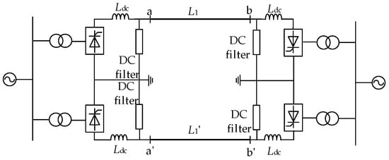
Figure 1.
The topology of the HVDC system.
Where a and b are the protection installations of the positive pole, a’ and b’ are the protection installations of the negative pole, and Ldc is the smoothing reactor.
When the system is in normal operation, the calculated value of remote end voltage can be calculated from the measured value of local end voltage. Since there is no fault branch and the line model is a faultless model, the measured value of the local end voltage is approximately equal to the calculated value of the remote end voltage. In this paper, rectifier LCC is used to realize characteristic signal injection to identify permanent faults. Before signal injection, it needs to be deionized by a fixed delay, so when a temporary fault occurs, the fault branch has disappeared at the time of signal injection. The line model after signal injection is consistent with the line model during normal operation of the system. At this time, the measured value of the local end voltage is approximately equal to the calculated value of the remote end voltage. The line model after the signal injection time in case of a temporary fault is shown in Figure 2, where R0, L0, and C0 are the resistance, capacitance, and inductance per unit length of the line, respectively.
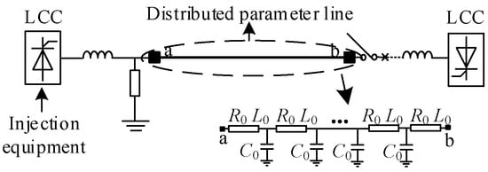
Figure 2.
Line model after signal injection with temporary fault.
As shown in Figure 2, in case of temporary fault, the LCC at the inverter side is bypassed and can be regarded as open-circuit after the fault occurs. Since the injection signal frequency is low (20 Hz), the capacitance branch to ground can be approximately open-circuit. At this time, there is no fault branch in the line, so there is no fault loop. So, the current in the line is 0 during the signal injection period, the injection voltage shows an upward trend, and the amplitude is large. The measured value of local end voltage and the calculated value of remote end voltage in case of temporary fault are shown in Figure 3, where uma is the measured value of local end voltage and ucb is the calculated value of remote end voltage.
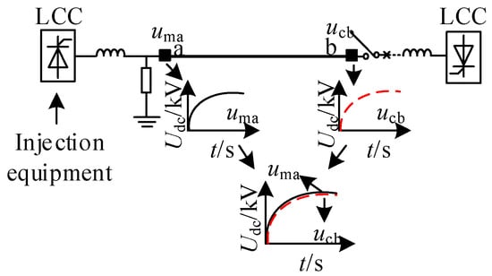
Figure 3.
Measured value of local end voltage and calculated value of remote end voltage with temporary fault.
When a permanent fault occurs, the fault branch still exists after signal injection. The line model is a fault model, and there is a large difference between the measured value of the local end voltage and the calculated value of the remote end voltage. The line model in case of permanent fault is shown in Figure 4, where Rf is fault resistance.
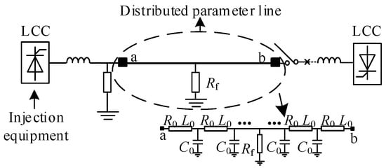
Figure 4.
Line model with permanent fault.
As shown in Figure 4, when a permanent fault occurs, the remote end and the capacitance branch to ground can be equivalent to an open circuit after the fault occurs. However, due to the existence of the fault branch, the current forms a loop with the ground through the fault branch. At this time, the current in the line is not 0, the injection voltage changes sinusoidally, and the voltage amplitude is low. The measured voltage at local end and the calculated voltage at the remote end are shown in Figure 5.
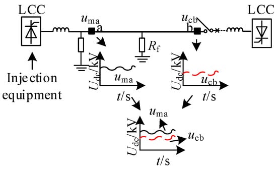
Figure 5.
Measured value of local end voltage and calculated value of remote end voltage with permanent fault.
To sum up, in case of temporary fault, since the fault branch does not exist after signal injection, the measured value of local end voltage is approximately equal to the calculated value of remote end voltage. Due to the existence of a fault branch after signal injection, there is a large difference between the measured value of local end voltage and the calculated value of remote end voltage with a permanent fault. In this paper, permanent fault identification is realized based on the difference between the measured value of the local end voltage and the calculated value of the remote end voltage.
3. Injection Signal Strategy
When the HVDC system operates normally, the LCC at the rectifier side adopts constant current control, and the inverter-side LCC adopts constant current control and extinction angle control. In case of DC line fault, the LCC at the rectifier side will conduct emergency phase shifting or change the reference value of constant current control [21] to realize fault current limiting, and the inverter-side LCC will be bypassed.
At present, there are few researches on using an LCC to realize characteristic signal injection, but there are also some papers that have carried out preliminary exploration. Refs. [18,19] inject current signals through LCCs, and [20] injects a voltage signal through an LCC. The control block diagram is shown in Figure 6.
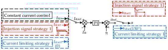
Figure 6.
Existing LCC injection signal control strategy.
Where Idcn is the DC current reference value of constant current control DC current during normal operation, Idc is the measured value of DC current, Idcset is the set value of DC current in [18,19]’s injection signal stage, Idcset1 is the set value of DC current in [18]’s fault current limiting stage, αref is the reference value of the trigger angle, αset is the set value of the trigger angle in [19,20]’s fault current limiting stage, αset1 is the set value of the trigger angle in [21]’s injection signal stage, and α is the trigger angle of the final output.
As shown in Figure 6, the LCC adopts constant current control during normal operation. After the fault occurred, [18] set the constant current control reference value to 0 to realize fault current limiting. Ref. [19] achieved fault current limiting by increasing the trigger angle to more than 90° through emergency phase shifting. After that, both of them inject current signals by changing the reference value of constant current control. Considering the unidirectional conductivity of the thyristor, in the current injection stage, to ensure the constant current direction, the DC component should be added to the DC current reference value of the above injection method, as shown in the following equation.
where A is the DC component; B is the injection signal amplitude; ω is the angular frequency of the injection signal; φ is the initial phase of the injection signal.
Ref. [20] realizes fault current limiting by emergency phase shifting and then realizes voltage signal injection by changing the trigger angle over a short time step.
When the LCC side adopts constant current control, the PI control is driven by the deviation between the DC current reference value and the measured value to adjust, so as to obtain the corresponding trigger angle α. Therefore, this paper realizes characteristic signal injection by changing the trigger angle of the LCC. Since the response characteristics of the AC signal system injected into the DC system are more obvious, the AC signal is injected by changing the trigger angle sinusoidally.
For the fault current limiting strategy, ref. [18] set the current reference value to 0 to achieve fault current limiting and then obtained the trigger angle through PI control. The control function is shown in the following equation.
where P is the proportional coefficient of PI regulator; T is the integral time constant of the PI regulator. Refs. [19,20] realize fault current limiting by directly changing the trigger angle, save PI control time, and can limit the fault current to 0 faster. The effects of the two different fault current limiting strategies are shown in Figure 7.
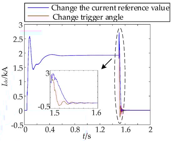
Figure 7.
Fault current limiting effect of different control strategies.
According to Figure 7, the fault current limiting strategy by changing the trigger angle can limit the current to 0 faster. Therefore, this paper realizes the fault current limiting by changing the trigger angle for emergency phase shifting.
To sum up, the LCC injection signal strategy adopted in this paper is shown in Figure 8.
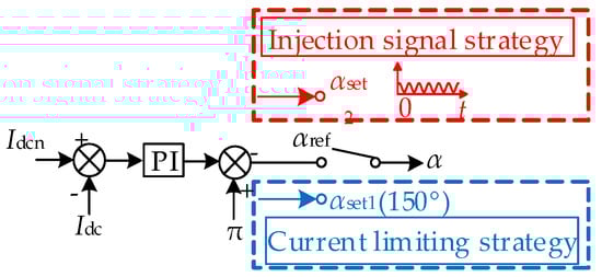
Figure 8.
Injection signal strategy of LCC.
Where αset1 is the trigger angle setting value in the fault current limiting stage, and αset2 is the trigger angle setting value in the injection signal stage.
For the LCC, pole-to-ground DC voltage Udc can be expressed as
where N is the number of 6 pulse converters in each pole, in this paper, 12-pulse converters are used, taking N = 2, U1 is the effective value of no-load line voltage at the valve side of converter transformer, which is 210 kv in this paper; α is the trigger angle; Xr is commutation reactance; Idc is DC current.
According to (3), the voltage signal can be injected by changing the trigger angle. Therefore, this paper uses voltage as the research object.
When a fault occurs, the LCC side triggers the fault current limiting strategy to limit the fault current to 0. In this paper, the trigger angle α is set to 150°, as shown in (4).
After the fault occurs, the system enters the system recovery stage after a fixed delay of 150 ms (i.e., the deionization time, generally 100 ms~300 ms) [22]. At this time, LCC switches from the fault current limiting control strategy to signal injection control strategy; that is, signal injection is realized by changing the trigger angle.
4. Injection Signal Selection
The injection signal selection needs to be considered from three aspects: injection length, injection frequency, and injection amplitude. The following is the specific analysis.
4.1. Length of Injection Signal
The length of the injection signal needs to consider factors such as signal transmission delay, signal sampling period, transformer transmission delay, etc. Specific analysis is as follows:
(1) Signal transmission delay: The wave speed of signal transmission is as follows [18].
According to (5), considering the total length of the line used in this paper is about 1500 km, the signal transmission time in the line is about 7.5 ms. The injection signal duration shall be greater than the signal transmission delay.
(2) Signal sampling period: According to the Nyquist theorem, to accurately extract the signal, it needs at least twice the length of the characteristic frequency. Considering that the injection signal frequency selected is 20 Hz in this paper, the sampling period is 50 ms, and the double length is 100 ms.
(3) Transformer transmission delay: The current national standard GB/T 26217-2019 stipulates that the transmission delay of DC electronic voltage transformers shall not be greater than 500 μs [23], and the injection time shall be greater than the transmission delay of the transformer.
(4) Filter delay: In this paper, a 50-order FIR low-pass filter is used to extract the time-domain waveform, and the filter delay calculation equation is shown in (6).
where n is the filter order; fs is the system sampling rate. According to (6), when the sampling rate of the system is 10 kHz, the filter delay is 5 ms, and the duration of the injected signal should be greater than the filter delay.
(5) The system recovers for a short time to improve the reliability of the power supply. The system should be recovered in a short time to reduce the power failure time, so the injection signal time should not be too long. During the recovery process of the project, the deionization time is generally set to 100~300 ms, and the number of restarts is set to 0~5. System recovery takes several seconds or even longer.
(6) Impact on the system: When the converter operates at a large trigger angle (above 50°), the operating conditions of the main equipment in the converter station deteriorate, the service life will be reduced accordingly, and the interference level of the converter station will also increase [24]. Therefore, the signal injection time should not be too long.
To sum up, to ensure the effect of the injection signal, the length of the injection signal is set to 150 ms.
4.2. Frequency of Injection Signal
When selecting the injection signal frequency, factors such as signal transmission effect, converter frequency output capability, DC filter resonance, and so on should be considered. Specific analysis is as follows:
(1) Signal transmission effect: The attenuation factor in the transmission process of the injection signal shall be considered, and the line transmission coefficient is shown in (7).
Considering that the length of the line used in this paper is about 1500 km, the typical transmission attenuation curve under a 1500 km overhead line is drawn according to (7), as shown in Figure 9.
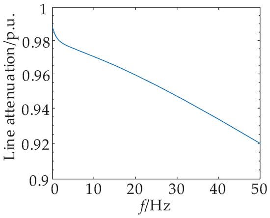
Figure 9.
Line transmission attenuation.
According to Figure 9, the higher the injection signal frequency, the more serious the signal attenuation, so the injection signal frequency should not be too high.
(2) Converter frequency output capability: In this paper, a 12-pulse converter is used, and the effect of signal injection at different frequencies is shown in Figure 10.
Figure 10.
Effect of different frequency injection signal.
According to Figure 10, the quality of the injection signal gradually deteriorates as the frequency increases, subject to the output capacity of the converter. At the same time, considering that the 12-pulse converter will output 12-time integer harmonics, the injected signal frequency should avoid the harmonic frequency.
(3) DC filter resonance: The injection signal frequency shall avoid the resonant frequency of the DC filter to avoid affecting the operation of the DC filter. Figure 11 shows the amplitude–frequency characteristic curve of the DC filter of the system in this paper.
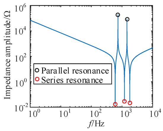
Figure 11.
Resistance–frequency characteristics of DC filter.
According to Figure 11, the DC filter has multiple series and parallel resonant frequencies, and the injection frequency should avoid the series and parallel resonant frequencies shown in Figure 11.
(4) Sampling rate of protection installation: In the actual project, the sampling rate of the protection installation is generally between 10 kHz and 50 kHz [9], and the injection frequency should be much lower than the sampling rate of the protection installation to ensure that the device can effectively obtain the injection signal.
(5) Considering that the distributed parameter model is used for analysis in this paper, the length of the line is 1500 km, so the amplitude–frequency characteristics of hyperbolic function under 1500 km are analyzed, and the amplitude–frequency characteristics are shown in Figure 12.
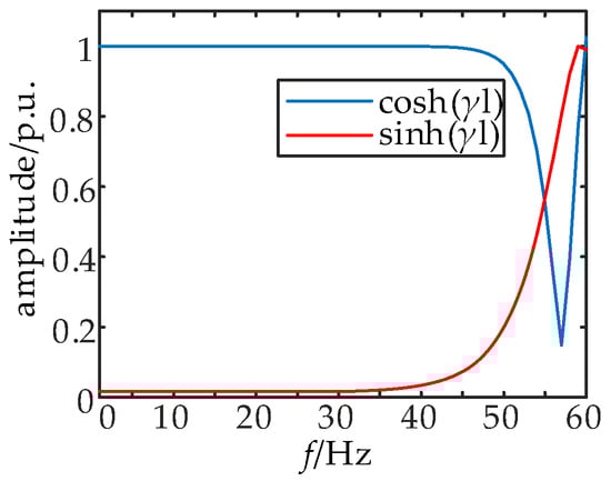
Figure 12.
Amplitude–frequency characteristics of hyperbolic function.
According to Figure 12, the hyperbolic function changes linearly in the low-frequency band. In addition, when using the distributed parameter model to calculate the electrical quantity at the remote end, only the line parameters of 100 Hz and below can be accurately calculated [25]. Therefore, the injection signal frequency should not be too high.
(6) Considering that this paper needs to calculate the voltage at the remote end from the voltage at local end, it is necessary to consider the distribution error along the voltage, as shown in (8) [26].
where ω is the angular frequency of the injection signal; l is the line length; v is the wave velocity. From (8), the error curve when the line length is 1500 km is shown in Figure 13.
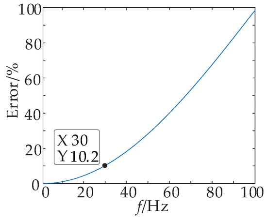
Figure 13.
Voltage distribution error along the line.
According to (8) and Figure 13, the error has reached 10.2% when the line length is 1500 km and the frequency is 30 Hz, and the error increases with the increase in frequency, so the injection frequency should not be too high.
(7) Impact on the system: The higher frequency of sine change trigger angle may cause the equipment to overheat for a short time and affect the stability of the system. Therefore, the frequency should not be too high.
To sum up, the frequency of the injection signal is 20 Hz.
4.3. Amplitude of Injection Signal
The amplitude of the injection signal needs to consider the measurement accuracy of the transformer, the impact on the injection equipment, and other factors. Specific analysis is as follows:
(1) Measurement accuracy of transformer: It must be ensured that the amplitude of the injection signal is greater than the lower limit of the measured value of the transformer. Taking the electronic transformer as an example, the amplitude of the injection signal should be greater than 0.05 p.u. [27]. According to (3), the change range of the trigger angle should be less than 87°, and the smaller the trigger angle, the higher the injection voltage amplitude, which will affect system operation. So, the trigger angle should not be too low. It is recommended to set the change range of trigger angle sine to 83~85°.
(2) Impact on injection equipment: Injection current will be generated in the DC line when the voltage signal is injected, resulting in the injection current component in the bridge arm. Because the smaller the trigger angle is, the higher the injection voltage amplitude is, the higher the injection current component amplitude is when the system resistance is constant.
The bridge arm current component is composed of the injection signal component and the original AC component. It shall be ensured that the bridge arm current does not exceed its maximum bearing range to avoid secondary impact on the equipment. The overload capacity of the thyristor for 5 s can reach 1.3 times the rated current [24]. The expression of bridge arm current is shown in (9).
When the system operates normally, the simulation results of rated DC current and rated AC current are shown in Figure 14.
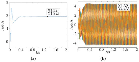
Figure 14.
Rated DC current and rated AC current during normal operation of the system. (a) Rated DC current. (b) Rated AC current.
According to Figure 14, the rated DC current is 1.923 kA and the rated AC current is 4.433 kA during normal operation of the system. According to Equation (9), the rated current of the bridge arm is about 2.86 kA. Because the overload capacity of the thyristor for 5S can reach 1.3 times the rated current, the maximum current that the bridge arm can withstand is about 3.718 kA.
When the sinusoidal change range of the trigger angle is 83~85°, the simulation results of DC current and AC current in the stage of signal injection under the most serious fault condition (i.e., DC line first end fault) are shown in Figure 15.
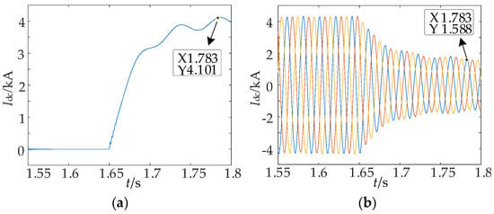
Figure 15.
DC current and AC current at LCC side during injection signal stage. (a) DC current. (b) AC current.
According to Figure 15, the bridge arm current reaches the maximum value when the DC current is 4.101 kA and the AC current is 1.588 kA. According to (9), the bridge arm current is about 2.161 kA, within its acceptable range. When the trigger angle continues to decrease, the DC peak current will increase, which may exceed the current bearing range of the bridge arm. Therefore, the trigger angle should not be too low.
To sum up, to ensure the effect of injection signal, the sine change range of the trigger angle is 83~85°.
The trigger angle and DC voltage response obtained by using the above injection signal length, frequency, and amplitude are shown in Figure 16.
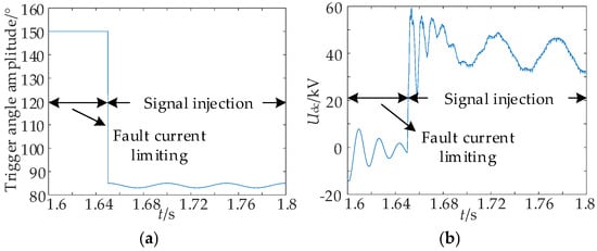
Figure 16.
Trigger angle and DC voltage response. (a) Trigger angle response. (b) DC voltage response.
From the above analysis, the injection method proposed in this paper does not need to be adjusted by PI and has a faster response speed.
5. Analysis of the Difference Characteristics of Injection Signals Under the Distributed Parameter Model
To improve the reliability of system recovery, it is necessary to identify the fault properties of the HVDC system. This section takes the L1 fault of DC line in Figure 1 as an example to analyze the differences under different fault properties after LCC signal injection.
5.1. Temporary Fault
The system in this paper is symmetrical bipolar, and the single pole grounding fault is analyzed as an example. After a fixed delay, the rectifier LCC switches from the fault current limiting control strategy to the injection signal control strategy. Due to the long DC transmission line, the influence of the distributed capacitive current cannot be ignored, so this paper introduces the distributed parameter model to analyze. In case of a temporary fault on L1, the equivalent circuit of distributed parameters is shown in Figure 17.
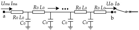
Figure 17.
Distributed-parameter equivalent circuit with temporary fault.
Where Uma and Ima are the measured values of voltage and current at terminal a in the injection signal stage, respectively; Ucb and Icb are the calculated values of voltage and current at terminal b in the injection signal stage, respectively; R0, L0, and C0 are the resistance, capacitance, and inductance per unit length of the line, respectively.
According to Figure 17, the measured value at terminal a and the calculated value at terminal b under temporary fault meet the following relationship.
where Zc is wave resistance; l is the total length of the line; γ is the propagation coefficient; and G0 is the conductivity per unit length of the line.
At this time, the amplitude difference between the measured value of terminal a voltage and the calculated value of terminal b voltage is shown in the following equation.
According to Figure 11, at the injection signal frequency (i.e., 20 Hz), cosh(γl) is about 1 and sinh(γl) is about 0. Therefore, considering the line loss, the relationship between the measured value of terminal a voltage and the calculated value of terminal b voltage can be obtained as follows.
Considering that, compared with the frequency domain algorithm, the calculation of the time domain algorithm is simpler and faster and the required data window length is shorter, the frequency domain distributed parameter model in (10) is converted to the time domain distributed parameter model, as shown in (14).
where uma(t) and ima(t) are the time domain information of voltage and current at the rectifier LCC side protection installation, respectively; v is the wave velocity, and its expression is v = 1/(L0C0)0.5.
The schematic diagram of the measured value of terminal a voltage and the calculated value of terminal b voltage in the time domain of a temporary fault are shown in Figure 18.
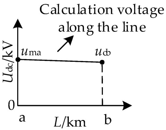
Figure 18.
Measured value of a end voltage and calculated value of b end voltage with temporary fault.
5.2. Permanent Fault
When a permanent fault occurs on line L1, its distributed parameter equivalent circuit is shown in Figure 19.
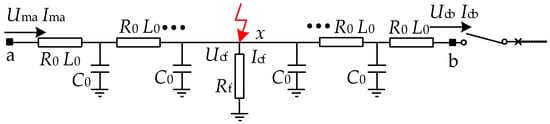
Figure 19.
Distributed-parameter equivalent circuit with permanent fault, where Ucf and Icf are the calculated values of voltage and current at the fault point when the permanent fault occurs, Rf is the fault resistance, and x is the fault location.
According to Figure 19, the calculated value of terminal b calculated from the fault point under permanent fault is shown in the following equation.
The following equation can be obtained by transforming (15).
It can be concluded that the measured value of terminal a voltage and the calculated value of terminal b voltage meet the following relationship.
The time domain expression of voltage under permanent fault is similar to that under temporary fault, which will not be repeated here.
The differences between the measured value of terminal a voltage and the calculated value of terminal b voltage in the case of a permanent metallic pole-to-ground (PTG) fault and through a resistance grounding fault are analyzed, respectively.
In case of permanent metallic PTG fault, the fault point is directly connected to the ground, as shown in Figure 20. Affected by the injection current at the fault point, the calculated value of terminal b voltage is true before the voltage is calculated to the fault point and then false. Its time domain schematic diagram is shown in Figure 21, where x is the fault location.
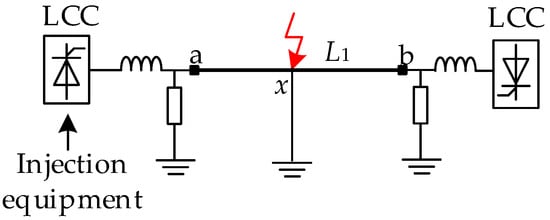
Figure 20.
System topology of permanent metallic PTG fault.
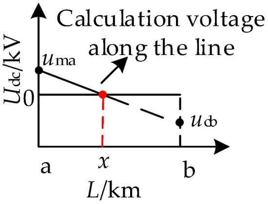
Figure 21.
Measured value of a end voltage and calculated value of b end voltage with permanent metallic PTG fault.
In case of permanent PTG fault through fault resistance, the system topology is shown in Figure 22. Because the fault resistance at the fault point supports the voltage, the higher the fault resistance is, the closer the calculated value of terminal b voltage is to the measured value of terminal a voltage. Similar to the metallic PTG fault, the calculated value of terminal b voltage is true before the voltage is calculated to the fault point and then false. Its time domain diagram is shown in Figure 23.
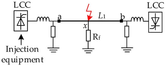
Figure 22.
System topology of permanent PTG fault with fault resistance.
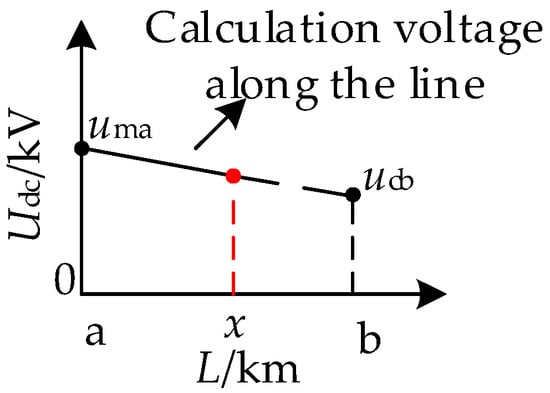
Figure 23.
Measured value of a end voltage and calculated value of b end voltage with permanent PTG fault with fault resistance.
In addition, due to the coupling between the positive and negative DC lines, it is necessary to conduct decoupling analysis on the positive and negative DC lines, calculate them in the mode domain, and finally obtain the phasor domain through decoupling inverse transformation. The 1-mode and 0-mode components after current and voltage decoupling at the protection installation are shown in the following equation.
where subscripts “1” and “0” denote 1-mode and 0-mode, respectively; “p” and “n” represent the electrical quantities of the positive and negative electrodes, respectively.
After the calculation, the maximum value is obtained through the decoupling inverse matrix shown in Equation (20).
6. Permanent Fault Identification Scheme
6.1. Fault Identification Scheme
According to the above analysis, the fault characteristics are determined when the temporary fault occurs, and the line model is a faultless model. Due to the line loss, the calculated value of the local end voltage is slightly lower than the measured value of the remote end voltage. In case of permanent fault, due to the existence of a fault branch, the transmission of electrical quantity is affected, and the fault characteristics are uncertain. The line model is a fault model, so there is a large difference between the measured value of local end voltage and the calculated value of remote end voltage, and the calculated value of remote end voltage is less than the measured value of local end voltage.
To sum up, considering the amplitude difference between the measured value of the local end voltage and the calculated value of the remote end voltage under different fault properties, this paper uses the absolute value of the area difference between the two (that is, the area of the shaded part in Figure 24 and Figure 25) to realize permanent fault identification.
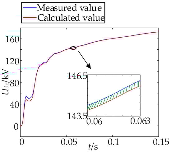
Figure 24.
Measured value of local end voltage and calculated value of remote end voltage with temporary fault.
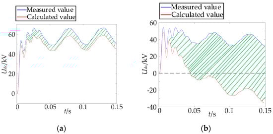
Figure 25.
Measured value of local end voltage and calculated value of remote end voltage with permanent fault. (a) Metallic PTG fault. (b) PTG fault through 400 Ω fault resistance.
To facilitate setting thresholds, normalize the time axis to 0~1, select the measured value of local end voltage as the standard, and normalize the DC voltage, as shown in the following equation.
where u’m and u’c are the measured value of local end voltage and the calculated value of remote end voltage after normalization, respectively, and um and uc are the measured value of local end voltage and the calculated value of remote end voltage before normalization.
The normalized area difference is defined as follows.
where Sm is the area of local voltage measurement value; Sc is the area of the calculated value of the remote end voltage; 0 is the start time of injection signal after normalization; 1 is the end time of injection signal after normalization.
Under temporary fault, the amplitude difference between the measured value of local end voltage and the calculated value of remote end voltage is small, and the normalized area difference S is small. Under permanent fault, the amplitude difference between the measured value of local end voltage and the calculated value of remote end voltage is large, and the normalized area difference S is large. Therefore, the permanent fault identification criteria can be obtained as follows.
where Sset is the threshold.
The transmission attenuation of the line will affect the transmission amplitude of the electrical quantity, so the selection and analysis of the Sset value considering its influence are as follows: when the line length is 1500 km, the transmission attenuation of the line is as shown in Figure 9. When the injection signal is 20 Hz and below, the amplitude attenuation of the line electrical quantity is less than 0.03 p.u. After normalization, the Sset value can be set to 0.03. In addition, considering a certain margin, set the reliability coefficient K = 1.2. The threshold Sset is shown in the following equation.
6.2. Flow Chart of Fault Identification Scheme
The flow chart of the permanent fault identification scheme is shown in Figure 26.
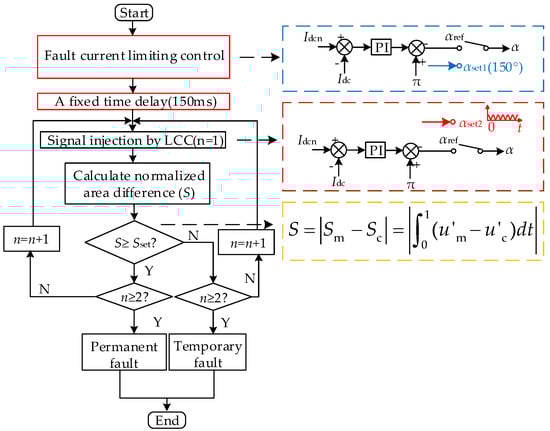
Figure 26.
Flow chart of permanent fault identification scheme.
After the fault occurs, the system switches to the fault current limiting control strategy. The emergency phase shift of the trigger angle at the LCC side is 150°, and after a fixed delay of 150 ms, the LCC switches to the injection signal strategy. The characteristic signal is injected by changing the trigger angle of the LCC, and then the normalized area difference S is calculated, which is compared with Sset to realize permanent fault identification. To improve the reliability of permanent fault identification, the signal can be injected multiple times. In this paper, the injection times are set as 2.
7. Simulation Verification
The electromagnetic temporary model of the HVDC system is established in PSCAD, and the permanent fault identification scheme is verified by MATLAB 2018b. The line is the frequency-dependent parameter model, and the system topology and specific parameters are shown in Figure 27 and Table 1, respectively. The time of fault occurrence is 1.5 s, the length of the temporary fault is 0.1 s, and the sampling rate of the system is 10 kHz.
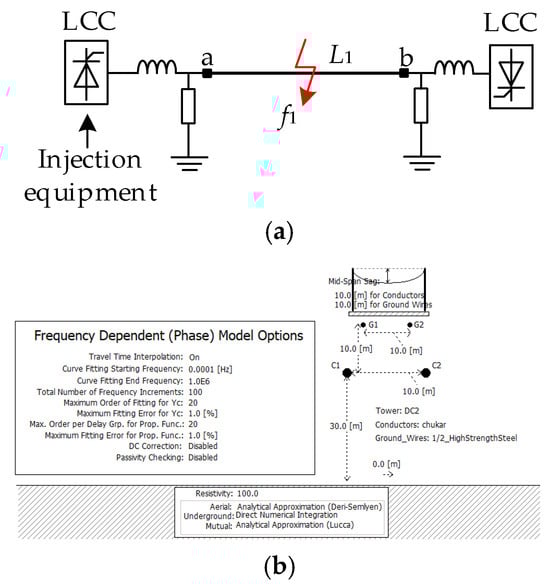
Figure 27.
The HVDC system. (a) Topology of HVDC system. (b) The frequency-dependent parameter model.

Table 1.
Parameters of HVDC system.
7.1. Analysis of Simulation Results of Permanent Fault Identification
Taking the pole-to-ground (PTG) fault as an example, the proposed permanent fault identification scheme is simulated and verified. Taking fault f1 on line L1 as an example, the fault on line L1 is 15 km, 375 km, 750 km, 1125 km, and 1485 km away from the a end (f15, f375, f750, f1125, f1485). For when faults occur in line L1, the measured voltage at the local end and the calculated voltage at the remote end are shown in Figure 28, Figure 29, Figure 30, Figure 31, Figure 32, Figure 33, Figure 34, Figure 35, Figure 36 and Figure 37. The permanent fault identification results are shown in Table 2. In Table 2, P represents a permanent fault and T represents a temporary fault.
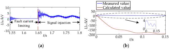
Figure 28.
Permanent PTG metallic fault (f15). (a) Effect figure of injection signal. (b) Measured value and calculated value.
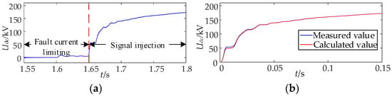
Figure 29.
Temporary PTG metallic fault (f15). (a) Effect figure of injection signal. (b) Measured value and calculated value.
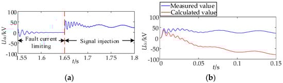
Figure 30.
Permanent PTG metallic fault (f375). (a) Effect figure of injection signal. (b) Measured value and calculated value.
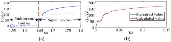
Figure 31.
Temporary PTG metallic fault (f375). (a) Effect figure of injection signal. (b) Measured value and calculated value.
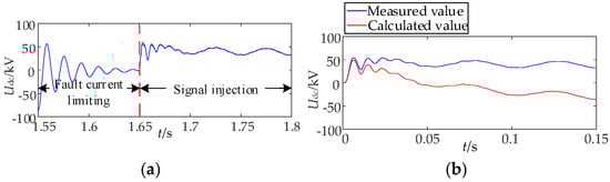
Figure 32.
Permanent PTG metallic fault (f750). (a) Effect figure of injection signal. (b) Measured value and calculated value.
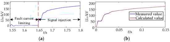
Figure 33.
Temporary PTG metallic fault (f750). (a) Effect figure of injection signal. (b) Measured value and calculated value.
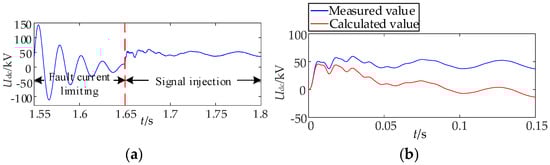
Figure 34.
Permanent PTG metallic fault (f1125). (a) Effect figure of injection signal. (b) Measured value and calculated value.
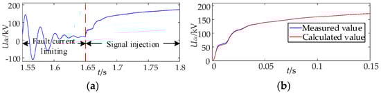
Figure 35.
Temporary PTG metallic fault (f1125). (a) Effect figure of injection signal. (b) Measured value and calculated value.
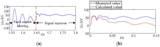
Figure 36.
Permanent PTG metallic fault (f1485). (a) Effect figure of injection signal. (b) Measured value and calculated value.
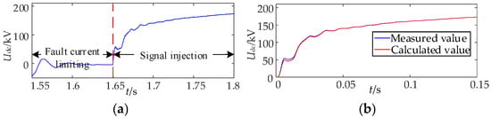
Figure 37.
Temporary PTG metallic fault (f1485). (a) Effect figure of injection signal. (b) Measured value and calculated value.
Table 2.
The identification results of the PTG metallic fault.
According to Table 2, the amplitude difference between the measured value of local end voltage and the calculated value of remote end voltage under permanent fault is large, and the normalized area difference is greater than 0.036. The amplitude difference between the measured value of local end voltage and the calculated value of remote end voltage under temporary fault is small, and the normalized area difference is less than 0.036. The proposed scheme can effectively identify a permanent fault and is not affected by the fault location.
7.2. Influence Analysis of the Proposed Scheme Under the PTG Fault with Fault Resistance
To fully verify the impact of fault resistance on the performance of the proposed method, take the PTG fault as an example. Set the fault resistance to be 100 Ω, 200 Ω, 300 Ω, and 400 Ω, respectively. Taking fault f1 on line L1 as an example, the fault on line L1 is 15 km, 375 km, 750 km, 1125 km, and 1485 km away from end a (f15, f375, f750, f1125 f1485). The permanent fault identification results are shown in Figure 38 and Figure 39.
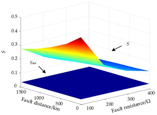
Figure 38.
Permanent fault.
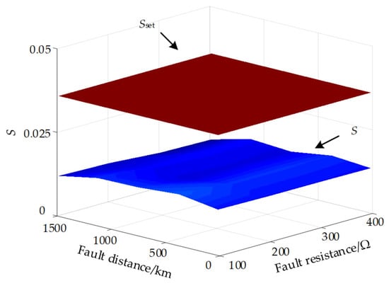
Figure 39.
Temporary fault.
7.3. Influence Analysis of the Proposed Scheme Under the PTG Fault with Noise Interference
To fully verify the impact of noise interference on the performance of the proposed method, take the PTG fault as an example, add noise with a signal-to-noise ratio (SNR) of 30 dB to the data, and set the fault resistance as 400 Ω. The fault on line L1 is 15 km, 375 km, 750 km, 1125 km, and 1485 km away from end a (f15, f375, f750, f1125, f1485). For when a fault occurs in line L1, the measured voltage at local end and the calculated voltage at the remote end are shown in Figure 40, Figure 41, Figure 42, Figure 43, Figure 44, Figure 45, Figure 46, Figure 47, Figure 48 and Figure 49, and the permanent fault identification results are shown in Table 3.
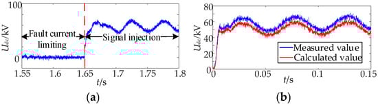
Figure 40.
Permanent PTG fault (add noise, f15). (a) Effect figure of injection signal. (b) Measured value and calculated value.
Figure 41.
Temporary PTG fault (add noise, f15). (a) Effect figure of injection signal. (b) Measured value and calculated value.
Figure 42.
Permanent PTG fault (add noise, f375). (a) Effect figure of injection signal. (b) Measured value and calculated value.

Figure 43.
Temporary PTG fault (add noise, f375). (a) Effect figure of injection signal. (b) Measured value and calculated value.
Figure 44.
Permanent PTG fault (add noise, f750). (a) Effect figure of injection signal. (b) Measured value and calculated value.
Figure 45.
Temporary PTG fault (add noise, f750). (a) Effect figure of injection signal. (b) Measured value and calculated value.
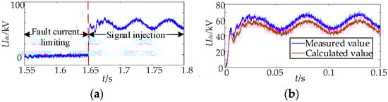
Figure 46.
Permanent PTG fault (add noise, f1125). (a) Effect figure of injection signal. (b) Measured value and calculated value.
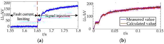
Figure 47.
Temporary PTG fault (add noise, f1125). (a) Effect figure of injection signal. (b) Measured value and calculated value.
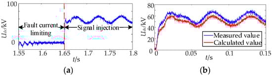
Figure 48.
Permanent PTG fault (add noise, f1485). (a) Effect figure of injection signal. (b) Measured value and calculated value.
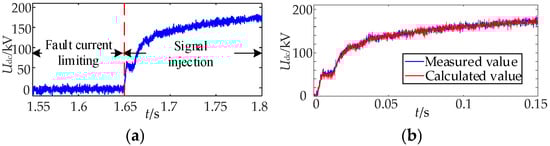
Figure 49.
Temporary PTG fault (add noise, f1485). (a) Effect figure of injection signal. (b) Measured value and calculated value.
Table 3.
The identification results with noise interference.
According to Figure 40, Figure 41, Figure 42, Figure 43, Figure 44, Figure 45, Figure 46, Figure 47, Figure 48 and Figure 49 and Table 3, the normalized area difference is greater than 0.036 for permanent faults and less than 0.036 for temporary faults. The proposed method can effectively identify permanent faults under 30 dB noise interference.
7.4. Influence Analysis of the Proposed Scheme Under the PTG Fault with Different Sampling Rates
To fully verify the impact of sampling rate on the performance of the method proposed in this paper, taking the PTG fault as an example, set the sampling rate to 5 KHz and 20 kHz, and set the fault resistance to 400 Ω. The fault on line L1 is 15 km, 375 km, 750 km, 1125 km, and 1485 km away from end a (f15, f375, f750, f1125 f1485). The permanent fault identification results are shown in Table 4.
Table 4.
The identification results with different sampling rates.
According to Table 4, the proposed method can effectively identify permanent faults under different sampling rates and is less affected by the sampling rate.
7.5. Influence Analysis of the Proposed Scheme Under the PTG Fault with Different DC Boundary
To fully verify the influence of boundary conditions on the performance of the method proposed in this paper, taking the PTG fault as an example, the smoothing reactor at the LCC side is set to 50 mh and 300 mh, respectively, and the fault resistance is set to 400 Ω. The fault on line L1 is 15 km, 375 km, 750 km, 1125 km, and 1485 km away from end a (f15, f375, f750, f1125 f1485). The permanent fault identification results are shown in Table 5.
Table 5.
The identification results with different DC boundary.
According to Table 5, the proposed method can effectively identify permanent faults under different boundary conditions and is less affected by the DC boundary attenuation effect.
7.6. Performance of Time-Varying Resistance
When arcing faults occur in a transmission line, the fault resistance can be approximately equivalent to time-varying resistance. Taking the PTG fault as an example to verify the performance of the proposed scheme under the time-varying fault resistances scenario, the fault of line L1 is 15 km, 375 km, 750 km, 1125 km, and 1485 km away from the a end, respectively (f15, f375, f750, f1125, f1485). The time-varying fault resistances is set as Rf = 200 + 50 t Ω (t > tfault, tfault is the time corresponding to the initial instant of the fault). The fault identification results are shown in Table 6.
Table 6.
The identification results of the PTG fault under time-varying fault resistances.
According to Table 6, the proposed fault identification scheme can effectively identify permanent and temporary faults under time-varying fault resistances, and it has certain dynamic fault resistance performance.
7.7. Compared with Existing Methods
The comparison between the proposed method and existing methods is shown in Table 7.
Table 7.
Comparison results with existing scheme.
According to Table 7, the existing permanent fault identification methods rely more on traveling waves, which are greatly affected by the sampling rate and DC boundary. The method of injecting signals using an LCC partially depends on simulation setting, while the method proposed in this paper is less affected by the sampling rate and DC boundary and does not need simulation setting.
8. Conclusions
For HVDC systems, a permanent fault identification scheme based on LCC injection signal is proposed in this paper. The main conclusions are as follows:
(1) The proposed scheme realizes fault current limiting through emergency phase shifting after a fault occurs and injects voltage signal through sinusoidal change of trigger angle after a fixed delay, without PI link control, and with faster response speed.
(2) The proposed scheme uses the amplitude difference between the measured voltage at the local end and the calculated voltage at the remote end under different fault properties to construct the normalized area difference to realize permanent fault identification, which only needs single end data, is not affected by data communication, and does not need simulation setting threshold.
(3) Simulation results show that the proposed scheme can withstand 400 Ω fault resistance and 40 dB noise interference and is less affected by fault distance, sampling rate, and DC boundary, and it has strong robustness.
(4) Future research paths include integration with machine learning for adaptive threshold tuning and hybrid LCC–MMC system validation under transient recovery states; applying digital twin technology to permanent fault identification; and research on an signal injection strategy for adaptive adjustment of injection start time.
Author Contributions
Conceptualization, Q.Z. and S.Z.; methodology, Q.Z.; validation, J.C.; formal analysis, J.Z.; investigation, L.Z. and S.Z.; resources, Q.Z.; data curation, J.T.; writing—original draft preparation, Q.Z.; writing—review and editing, J.T.; visualization, Q.Z.; supervision, J.C.; project administration, J.Z.; funding acquisition, Q.Z. All authors have read and agreed to the published version of the manuscript.
Funding
This work has been supported by the State Grid Xinjiang Electric Power Research Institute Technology Project (DQ30DK24001H).
Data Availability Statement
The original contributions presented in the study are included in the article. Further inquiries can be directed to the corresponding author.
Conflicts of Interest
The authors declare that the research was conducted in the absence of any commercial or financial relationships that could be construed as a potential conflict of interest.
Correction Statement
This article has been republished with a minor correction to the Funding statement. This change does not affect the scientific content of the article.
References
- Chen, N.; Zha, K.P.; Qu, H.T.; Li, F.L.; Xue, Y.; Zhang, X.P. Economy Analysis of Flexible LCC-HVDC Systems with Controllable Capacitors. CSEE J. Power Energy Syst. 2022, 8, 1708–1719. [Google Scholar] [CrossRef]
- Niu, S.; Jia, Q.; Hu, Y.; Yang, C.; Jian, L. Safety Management Technologies for Wireless Electric Vehicle Charging Systems: A Review. Electronics 2025, 14, 2380. [Google Scholar] [CrossRef]
- Chen, Y.; Xu, L.; Egea-Alvarez, A.; Marshall, B. Accurate and General Small-Signal Impedance Model of LCC-HVDC in Sequence Frame. IEEE Trans. Power Deliv. 2023, 38, 4226–4241. [Google Scholar] [CrossRef]
- Chen, Z.Y.; Huang, H.Z.; Wu, J.; Wang, Y.H. Zero-faulty sample machinery fault detection via relation network with out-of-distribution data augmentation. Eng. Appl. Artif. Intell. 2025, 141, 109753. [Google Scholar] [CrossRef]
- Chen, Z.Y.; Huang, H.Z.; Deng, Z.W.; Wu, J. Shrinkage mamba relation network with out-of-distribution data augmentation for rotating machinery fault detection and localization under zero-faulty data. Mech. Syst. Signal Process. 2025, 224, 112145. [Google Scholar] [CrossRef]
- Shu, H.C.; Cao, Y.R.; Dai, Y.; An, N. An Adaptive Reclosing Scheme for Flexible DC Ring Grid Based on Residual Voltage Waveform Offset Detection. IEEE Trans. Ind. Electron. 2024, 71, 7829–7838. [Google Scholar] [CrossRef]
- Zhang, D.H.; Liang, C.G.; Li, M.; Luo, Y.P.; Chen, K.; Mirsaeidi, S.; He, J.H. Voltage frequency-based adaptive reclosing strategy for flexible DC power grids. Int. J. Electr. Power Energy Syst. 2021, 131, 10. [Google Scholar] [CrossRef]
- Yu, J.Q.; Zhang, Z.R.; Xu, Z. Adaptive sequential reclosing strategy for hybrid HVDC circuit breakers in MMC-based DC grids. High Volt. 2022, 7, 890–902. [Google Scholar] [CrossRef]
- Wang, T.; Song, G.B.; Hussain, K.S.T. Adaptive Single-Pole Auto-Reclosing Scheme for Hybrid MMC-HVDC Systems. IEEE Trans. Power Deliv. 2019, 34, 2194–2203. [Google Scholar] [CrossRef]
- Hou, J.J.; Song, G.B.; Sun, Y.; Fan, Y.F.; Wu, X.F.; Chang, P.; Chang, N.N. Permanent fault identification and location scheme for MTDC grid based on equivalent impedance phase characteristics and distributed parameter line. Int. J. Electr. Power Energy Syst. 2023, 153, 16. [Google Scholar] [CrossRef]
- Cai, P.C.; Xiang, W.; Zhou, M.; Ni, B.Y.; Wen, J.Y. Research on Adaptive Reclosing of DC Fault Based on Active Signal Injected by Hybrid MMC. Proc. CSEE 2020, 40, 3867–3878. [Google Scholar]
- Li, Z.; Zheng, Y.C.; Lin, X.N.; Tong, N.; Wei, F.R.; Xiao, S.Y. Adaptive Reclosing Scheme for VSC-MTDC Line Based on the Transient Current Waveform Similarity Matching. High Volt. Eng. 2023, 49, 1326–1339. [Google Scholar]
- Yang, S.Z.; Xiang, W.; Yang, R.Z.; He, Y.J.; Wen, J.Y. Research on Adaptive Reclosing Technology for the Half-bridge MMC and Hybrid DC Circuit Breaker Based on HVDC Systems. Proc. CSEE 2020, 40, 4440–4451+4724. [Google Scholar]
- Mei, J.; Ge, R.; Zhu, P.F.; Fan, G.Y.; Wang, B.B.; Yan, L.X. An Adaptive Reclosing Scheme for MMC-HVDC Systems Based on Pulse Injection From Parallel Energy Absorption Module. IEEE Trans. Power Deliv. 2021, 36, 1809–1818. [Google Scholar] [CrossRef]
- Han, P.; Zhao, X.C.; Wu, Y.N.; Zhou, Z.Y.; Qi, Q. Adaptive Reclosing Scheme Based on Traveling Wave Injection For Multi-Terminal dc Grids. Energy Eng. 2023, 120, 1271–1285. [Google Scholar] [CrossRef]
- Zhang, S.; Zou, G.B.; Xu, C.H.; Sun, W.J. A Reclosing Scheme of Hybrid DC Circuit Breaker for MMC-HVdc Systems. IEEE J. Emerg. Sel. Top. Power Electron. 2021, 9, 7126–7137. [Google Scholar] [CrossRef]
- Zhang, D.H.; Yang, Y.C.; Liang, C.G.; Li, M.; Liu, Y.M.; He, J.H. Adaptive Reclosing Scheme for Flexible DC Power Grid Based on Improved DC Circuit Breaker Injecting Signal. Autom. Electr. Power Syst. 2022, 46, 123–132. [Google Scholar]
- Xu, R.D.; Song, G.B.; Hou, J.J.; Chang, Z.X. Adaptive restarting method for LCC-HVDC based on principle of fault location by current injection. Glob. Energy Interconnect. 2021, 4, 554–563. [Google Scholar] [CrossRef]
- Hou, J.J.; Song, G.B.; Fan, Y.F. Fault properties identification scheme for hybrid MTDC system based on LCC signal injection and distributed parameter line model. IET Gener. Transm. Distrib. 2023, 17, 3718–3738. [Google Scholar] [CrossRef]
- Liang, C.G.; Zhang, D.H.; Li, M.; Nie, M.; Mirsaeidi, S.; Xu, Y.; He, J.H. Waveform Difference Based Adaptive Restart Strategy for LCC-MMC Hybrid DC System. IEEE Trans. Power Deliv. 2022, 37, 4237–4247. [Google Scholar] [CrossRef]
- Wang, L.; Sun, X.F.; Wang, B.C.; Zhao, W.; Li, X. Research on Protection Scheme of DC Line Fault in LCC-MMC Hybrid HVDC System. Proc. CSEE 2021, 41, 7339–7352. [Google Scholar]
- Hou, J.J.; Song, G.B.; Fan, Y.F. Fault identification scheme for protection and adaptive reclosing in a hybrid multi-terminal HVDC system. Prot. Control Mod. Power Syst. 2023, 8, 17. [Google Scholar] [CrossRef]
- Zhu, M.M.; Wang, D.; Liao, Y.H.; Cao, P.L.; Shu, H.C.; Yang, B.; Duan, R.M. Field test and analysis of delay characteristics of a DC electronic voltage transformer. Power Syst. Prot. Control 2023, 51, 126–132. [Google Scholar]
- Zhao, W.J.; Xie, G.E.; Zeng, N.C. High Voltage Direct Current Transmission Engineering Technology, 2nd ed.; China Electric Power Press: Beijing, China, 2011; pp. 60–77. [Google Scholar]
- Song, G.B.; Rao, J.; Gao, S.P.; Cai, X.L.; Suo, N.J.L. Monopole Protection for HVDC Transmission Lines Based on Compensating Voltage. Autom. Electr. Power Syst. 2013, 37, 102–106+113. [Google Scholar]
- Zheng, J.C.; Wen, M.H.; Chen, Y.; Shao, X.N. A novel differential protection scheme for HVDC transmission lines. Int. J. Electr. Power Energy Syst. 2018, 94, 171–178. [Google Scholar] [CrossRef]
- Wang, P.; Zhang, G.X.; Li, L.Z.; Zhu, X.M.; Luo, C.M. Error analysis of electronic instrument transformers. J. Tsinghua Univ. (Sci. Technol.) 2007, 47, 1105–1108. [Google Scholar]


Disclaimer/Publisher’s Note: The statements, opinions and data contained in all publications are solely those of the individual author(s) and contributor(s) and not of MDPI and/or the editor(s). MDPI and/or the editor(s) disclaim responsibility for any injury to people or property resulting from any ideas, methods, instructions or products referred to in the content. |
© 2025 by the authors. Licensee MDPI, Basel, Switzerland. This article is an open access article distributed under the terms and conditions of the Creative Commons Attribution (CC BY) license (https://creativecommons.org/licenses/by/4.0/).