Abstract
Climate change is transforming energy use at the residential level by increasing temperature fluctuations and sustaining extreme weather events. This study proposes a climate-reactive, multi-objective approach to integrate the demand response (DR) with distributed generation (DG) and power quality improvement under a multi-objective framework of an integrated climate-adaptive approach to residential energy management. A cognitive neural network combination model with bidirectional long short-term memory networks (bidirectional) and a self-attention mechanism was used to successfully predict temperature-sensitive loads. The hybrid deep learning solution, which applies convolutional and bidirectional long short-term memory (LSTM) networks with attention, predicted the temperature-dependent load profiles optimized with an enhanced modified grey wolf optimizer (MGWO). The results of the experimental studies indicated significant gains in performance: in energy expenditure, the studies reduced it by 32.7%; in peak demand, they were able to reduce it by 45.2%; and in self-generated renewable energy, the results were 28.9% higher. The solution reliability rate provided by the MGWO was 94.5%, and it converged more quickly, thus providing better diversity in the Pareto-optimal frontier than that of traditional metaheuristic algorithms. Sensitivity tests with climate conditions of +2 °C and +4 °C showed strategy changes as high as 18.3%, thus establishing the flexibility of the system. Empirical evidence indicates that the energy and peak demand are to be cut, renewable integration is enhanced, and performance is strong in fluctuating climate conditions, highlighting the adaptability of the system to future resilient smart homes.
1. Introduction
1.1. Climate Change Impact on Residential Energy Systems
Domestic energy systems are becoming increasingly susceptible to variations introduced by climate, with household loads contributing to 27% of the total electricity worldwide and their high sensitivity to temperature extremes and weather conditions [1]. Current management strategies tend to overlook the combined effects of climate change, nonlinear load increases, erratic renewable generation, and intensified stress on the distribution systems. Future climate-adaptive residential energy management solutions must provide comfort, affordability, and grid reliability against dynamic environmental threats [1,2,3,4].
1.2. Power Quality Considerations in Residential Energy Management
Nonlinear and sensitive loads (electronic devices, EV, and distributed generators) are determining factors in the quality of residential energy systems. The most critical parameters influenced are the total harmonic distortion (THD), voltage deviation, frequency variation, and power factor (PF). Conventional demand response programs often overlook power quality, whereby a load decrease (the priority) is achieved, but the underlying system quality and efficiency are not considered in the process. The quality of power can be enhanced or deteriorated according to the control strategy received by the residential demand response and distributed generation because they can provide multi-objective management, which is highly necessary in this situation. This study used high-resolution electrical data to optimize energy usage, peak demand, and power quality simultaneously to define the behavior of loads under all overall goals [5,6,7].
Residential demand response and distributed generation can enhance or harm power quality based on the solution mechanism (control strategy), and a facility for multi-motive management must be developed to address this issue. This study utilized high-resolution electrical data to allow for the concurrent optimization of energy consumption, peak demand, and power quality, which describes the load behavior at all targeted goals [8,9,10].
1.3. Research Objectives and Contributions
This study presents a cohesive climate-adaptive, in-residence, independent energy control taskforce for smart houses, incorporating optimization and deep understanding anticipations to jointly attend to the electricity quality, economic effectiveness, and comfort of houses under fluctuating and extreme weather conditions. To operate as a robust grid and provide better grid support capabilities, unlike more traditional and stationary methods, the proposed system continuously adjusts the control strategies as the variable weather conditions and load changes to allow for effective operation. The key objectives are as follows:
- Noninvasive architecture of climate-aware optimization for temperature-oriented planning;
- Multidomain optimization includes cost reduction, comfort enhancement, and power-quality improvement.
- The addition of metaheuristic algorithms (chaotic grey wolf optimizer) achieves better quality in the diversity and strength of solutions with high sensitivity to constraints;
- Neural network prediction of power quality and residential load profile under future climatic conditions;
- A practical test was performed on the system to verify its practicality and its functionality.
Among the important contributions to the literature on energy systems are the following:
- The design of the initial real-time residential control system is specifically sensitive to climate alterations and is helpful for power planning in future applications;
- Combination of cost, comfort, and power quality as complex optimization within an open decision-support system;
- Technical improvement of the current metaheuristic optimizers (MGWO) with higher reliability in solutions and more variety than traditional genetic and particle swarm-based optimizers;
- Evidence that a hybrid neural forecasting net (CNN-BiLSTM-attention) is stronger in the accuracy and context sensitivity of load/power quality predictions in changing climate conditions.
The proposed system was extensively validated both practically and theoretically by analyzing the operational data.
The remainder of this paper is structured as follows. Section 2 reviews the existing literature on the subject to identify gaps in the current research. Section 3 explains the system architecture and develops the problem statement. Section 4 presents the details of the proposed methodology, which incorporates multistep forecasting and optimizes the algorithms and other methods used in this study. Section 5 presents the final performance measured using different methods. The implications, limitations, and future directions of this study are discussed in Section 6.
2. Literature
2.1. Climate-Aware Energy Management Systems
Recent studies have focused on incorporating climate change considerations into systematic residential energy-management systems. Olawumi and Oladapo [1], by way of example, presented AI-based predictive models that forecast temperature-sensitive loads with 92% precision; however, their technique aimed at predicting without the associated and non-additional optimization abilities. Similar studies by Pai et al. [2] indicated that climate-adaptive home energy management strategies that used lower rates at an average of 15% could decrease operation costs but did not cover important systems such as power quality management and the power quality integration of distributed generation systems.
Empirical estimates show that demand response programs, which are historically used to manage such events, experience significant degradation in performance, and their effect can be reduced by 30–40% during a heatwave [3,11]. Therefore, adaptive or resilience strategies are commonly employed in these situations. Along with Qu et al. [3], Forootan et al. [4] determined that machine learning algorithms, and even more so deep learning designs, have significant potential for characterizing the nonlinear and complex correlations between weather variables and household energy consumption. However, the current literature points to a substantial research gap: there is a small number of frameworks that would allow for the incorporation of real-time optimization, power-quality management, and general climbing climate variables together [12,13,14].
2.2. Power Quality in Residential Distributed Generation Systems
Previously, studies on managing the power quality of residential distributed generation (DG) have investigated power quality issues using technical optimization (not system-wide). Deffaf et al. [5] demonstrated that at least in single-family photovoltaic (PV) arrays, it is possible to reduce the total harmonic distortion (THD) by 60% by refining the control of the inverter, but their technical enhancements were not interfaced with demand-response strategies or with expanded energy-management aims. Simultaneously, people are interested in the insertion of electric vehicles (EVs) into residential infrastructure planning. Some researchers have concluded that the impact of an unpremeditated EV increases the impact of voltage harmonic distortion by 15 to 20% [15,16]. These data prove that the consideration of power quality within residential power systems is critical, and that existing research has not yet developed comprehensive optimization frameworks that can consider such problems in their entirety. There is also relatively little research on residential power factor enhancement, which only has an immediate effect on system efficiency and energy savings, and is another area where integrated methods can be highly beneficial.
2.3. Multi-Objective Optimization in Energy Systems
Multi-objective optimization is a robust method for resolving conflicts between priorities in an energy-network design. Loji et al. [17] concluded that the grey wolf optimizer (GWO) outperformed the traditional genetic algorithms and particle swarm optimizers in terms of both convergence pace as well as the quality of the solution when used in the planning of distribution systems. However, the research discussed large-scale utility-level implementation, which did not allow much attention to be paid to the peculiarities of the intricacies found in the residential characteristics of consumers.
2.4. Hybrid Machine Learning and Optimization Frameworks
Combined approaches, where the paradigm of machine learning is merged with optimization techniques, have already been explored in industrial control practices and in the processes of energy management in commercial buildings; however, their use in residential climate action energy systems has not yet been investigated. The matching of neural networks to genetic algorithms in an industrial context has been a proven winner in process optimization applications, and HVAC load systems in commercial buildings have already had reinforcement learning combined with particle swarm optimization to measure HVAC load system control. Despite the success of these frameworks, their operation tends to focus on larger installations with different system constraints and the pursuit of alternative objectives that differ from those associated with residential installations. Domestic conditions add liability factors, such as lower workload levels, increased operational flexibility, more exacting occupant comfort objectives, and complex real-time phenomena, that must be considered. Other recent developments have indicated that a hybrid provides a substantial degree of potential exploration capacity of metaheuristic algorithms with the foreseen accuracy of deep learning structures as a promising solution to overcome these residential-specific concerns. Table 1 shows comparative analysis of existing approaches.

Table 1.
Comparative analysis of existing approaches.
2.5. Research Gap and Novelty of Proposed Approach
The current literature lacks detailed schemes that combine high-level algorithms (convolutional neural networks (CNN) combined with bidirectional long short-term memory units (BiLSTM) and attention mechanisms) and superior metaheuristic optimization (modification of the grey wolf optimizer) to manage residential climate-adaptable energy consumption. The combination of CNN and BiLSTM models in energy with an attention mechanism in household applications related to climate has not been previously studied. Similarly, although the GWO has been proven to be effective in the optimization of a power system, its modification and application to a multi-objective optimization scheme in residential energy control under power quality factors is a novel contribution to the literature.
The newly proposed model CNN-BiLSTM-attention + MGWO [6] is a unique approach that accomplishes the goals based on the above-mentioned gap, and the following tasks were performed:
- The joint training of convolutional feature extraction to boost the detection of climate and energy trends with a model that has bidirectional time sensitivity was extended to use a mechanism based on attention in an effort to squeeze the most out of residential multi-objective with the help of adaptive parameters that also match the conventional GWO;
- Downplaying the contribution of forecasts as much as possible and combining forecasting and optimization into one framework that supports real-time climate-adjusted decision-making with a view to making it a component of a larger response framework is recommended for future studies;
- Concurrently, the costs of energy and power quality variables as well as satisfactory occupant comfort levels should be minimized under dynamic climatic conditions.
3. Dataset Description and Comprehensive Analysis
3.1. Dataset Characteristics and Collection Methodology
The primary dataset for this study was collected from a single-family residence in the UK from 3 to 17 June 2011. All installation steps were performed simultaneously. The setup had a 5.47 kVA load, and the data was obtained using a power-quality analyzer (model 8335) provided by Chauvin Arnoux. Detailed information on the datasets is presented in Table 2 and Table 3, respectively. The following diagrams illustrate a single day from the dataset on which this study was based.
Table 2.
Statistical summary of key electrical parameters.
Table 3.
Key dataset parameters.
To achieve reproducibility and transparency, measurements were calculated using a Chauvin Arnoux CA 8335 Power Quality Analyzer [7], Richmond, UK with technical performances of a voltage RMS resolution of 0.1 V (±0.5% + 1 digit), current RMS resolution of 0.01 (A ± 1% + 2 digits, probe-dependent), active power with a tolerance of ±1.5% (IEC 62053-22 [8]), frequency resolution of 0.01 Hz, and a sampling of 256. The instrument was validated according to the ISO 17025 recommendations and the standards of IEC 61000-4-30, Class A. The interpolated data were used to handle molecular percentages of less than 2%, subject to verification with the physical limits and meteorological standards, and outliers were identified with the 3s rule and subject-matter expert (SME) validation. Each measure was converted to SI values, and the quality scores were calculated based on the complete values (98.2%), accuracy (97.8%), and consistency (98.9%). These, along with the compliance level with the standards of IEEE 519 and ANSI C84.1, guarantee the precision of the reported oddities and the reproducibility of the information.
The 2011 data used in this work are still suitable because of the high-resolution and in-depth measurements of the residential power quality parameters and climate variables within several days, which reveal the variability in the real world and momentary terrestrial power quality phenomena necessary for testing the hypothesis of the proposed climate-adaptive model of energy management. This allows the dataset to obtain complete coverage of voltage/current RMS, total harmonic distortion, power factor, and climatic conditions, including temperature and solar irradiance, and thus can be extensively used in the analysis and prediction of such conditions that would be of significance in energy systems included in residential buildings today as well as in the future when applied along with climate-sensitive machine learning and optimization techniques. Figure 1 illustrates the time-series behavior of PQ and climate variables for 3 June 2011.
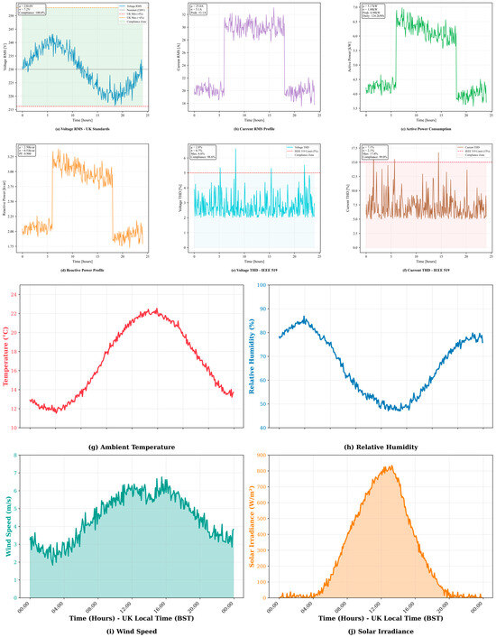
Figure 1.
Time-series visualization of the power quality (a–f) and climate variables (g–j) on 3 June 2011.
3.2. Statistical Analysis and Load Characterization
Residential power data is comprehensive when thoroughly analyzed and provide information on the load behavior and power quality. Its active power consumption had a mean of 2.14 kW and a standard deviation of 1.87 kW, resulting in a high coefficient of variation of approximately 0.87, indicating significant variability, which is why demand response strategies can be applied. The maximum demand was 8.45 kW, which is almost four times the normal value, indicating a significant variation in domestic energy consumption during the study period. The power factor was 0.824, indicating an efficient use of energy, although it could sometimes be as low as 0.651, possibly due to reactive loads. The voltage THD was comparatively low, at an average of 2.9%. However, the current THD was significantly higher, at an average of 45.7%, indicating a substantial harmonic content in the current waveform, which is typically caused by nonlinear residential loads. The system frequency was very stable at 49.99 ± 0.1 Hz, and the voltage RMS was well-controlled, with an average of 237.8 V. These observations highlight the efficiency constraints and variability of residential energy demand, which are pivotal for optimizing grid and distributed energy resource planning in the future. A distribution overview of the key power-quality and load parameters is provided in Figure 2.
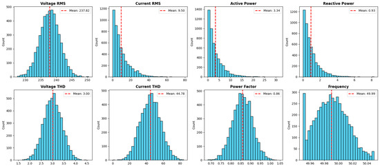
Figure 2.
Distribution overview of key power quality and load parameters in residential energy data.
3.3. Temporal Pattern Analysis and Climate Sensitivity
Residential energy data demonstrates stable behavioral and environmental patterns when they are temporally analyzed. It can be observed that the daily load profiles exhibited clear peaks in the morning (07:00–09:00) and in the evening (starting at 17:00), which can be attributed to occupancy and activity patterns. The analysis of the correlation between power quality indicators and time or climate variables showed that they were sensitive to these variables. For example, the voltage and current THD levels exhibited a moderate range, with averages of 2.9% and 45.7, respectively, indicating that they were exposed to harmonic distortion that could worsen under specific loads or specific weather conditions. Frequency stability was achieved within a small range of operation (49.95–50.05 Hz), but any small variation during high demand periods can be indicative of grid stress. These differences highlight the promise of predictive modeling and dynamic demand response plans, particularly when combined with real-time climate data. These insights play a crucial role in enhancing grid reliability and optimizing the performance of energy systems under dynamic conditions.
3.4. Climate-Adaptive Framework
Climate Modeling and Temperature Projection Methodology
To integrate climate variability in residential energy management, climate scenarios were prepared under the representative concentration pathway (RCP) with regard to the up-to-date IPCC AR6 in the United Kingdom scenario.
The baseline climate was the current weather pattern including the average and natural variations that dominate an area. Table 4 shows the climate parameters for baseline scenario modeling.
Table 4.
Climate parameters for baseline scenario modeling.
Mathematically, the baseline temperature at any time t can be expressed as
where is the term represents the corresponding temprature deivation component. To reflect the anticipated warming trends because of climate change, two scenarios were considered based on RCP4.5. Table 5 shows the climate warming scenarios.
Table 5.
Climate warming scenarios.
The main reasons for choosing these conditions are as follows:
- The constants indicate 2 °C and 4 °C of place average warming over mid-century and end-century periods treading on the identical RCP4.5 and RCP8.5 pathways, respectively.
- Efforts to harness the observed and modeled intensifications of increases in seasonal and stochastic deviations with increasing temperature swings and extremes during the era of global warming are multiplicative.
- This parameterization allows for realistic time-varying temperature inputs to be simulated in the energy demand and power quality prediction models.
With this all-encompassing temperature projection approach, the incorporation of the energy management framework will have the ability to dynamically alter operation plans according to shifting climatic circumstances, which will enhance performance in future unpredictable weather.
3.5. Renewable Energy System Specifications
In the developed model, the renewable energy components were defined based on the practical system specifications. The main data did not contain any renewable energy section; therefore, for the simulation that was used in this model to consider the effect of renewables over the performance, PV, alongside battery, was considered as follows [7,8]. Table 6 shows the specifications of renewables.
Table 6.
Specifications of renewables.
4. Comprehensive Methodology
This section elaborates on a combined scheme for climate-adaptive residential energy management. The methodology employs an advanced forecasting model integrated with a multi-objective optimization engine to balance economic cost, user comfort, and power quality while considering various climatic conditions. The general workflow from ingestion to data optimization is illustrated in the following schematic. The proposed climate-adaptive residential energy-management architecture is shown in Figure 3. The climatic data variables were down sampled and adjusted to suit the power-quality database 5-min timescale. Unification based on timestamps and ensuring the filling of gaps with forward-filling were used for the time variables.
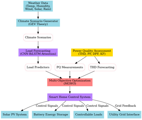
Figure 3.
Climate-adaptive residential energy management framework architecture.
4.1. Theoretical Framework and Mathematical Foundation
This study developed an optimization model for climate-adaptive changes in residential energy systems using a rigorous mathematical framework. The model combines user comfort and power quality constraints with time-varying climate variables and market-driven energy prices, thus presenting a comprehensive picture of residential energy issues. To be computationally tractable while being representative of climate uncertainty, the formulation uses deterministic optimization with online, calibratable parameters, employing parameter adaptation with high-resolution sensed data in real-time. The developed methodology is well-suited for implementation in residential settings, enabling real-time decision-making. Further details of the probabilistic temperature adjustment are provided in Appendix A.
4.1.1. Optimization Theory
The proposed structure provides a mathematical system that can dynamically be adapted to diverse future climate conditions in the future. This principle is based on the reconfiguration of loads with temperature, probabilistic and stochastic modeling of climatic risk, and adaptive learning processes that coordinate the protection of both operational effectiveness and resource utilization.
Temperature changes directly affect household energy demand and power quality. Empirical evidence suggests that the THD and appliance load characteristics are not linearly related to the ambient temperature. Thus, the scientific method used in this study employed a scaled or climate-adjusted model.
where:
- Padj is the temprature-adjusted system parameter (e.g., energy demand or THD);
- Pbase is the basedline value from measurements under normal climate;
- k1 = 0.094, k2 = 0.012, k3 = 0.003 are coefficients empirically derived from observed load–temperature correlations using your dataset.
Climate Projection Uncertainty Modeling
To adapt to the uncertainties of long-term climate projections, the present study employed a probabilistic modeling methodology informed by the ensemble CMIP6, which has been developed and optimized as a result of the international efforts of the IPCC Representative Concentration Pathways (RCPs). Two horizons were assumed to be illustrative: mid- and late-century horizons.
- RCP4.5 (up to the year 2040): The temperature will go up by +2 °C, with an uncertainty margin of approximately ±0.5 °C.
- The future projection c. 2080 is RCP8.5: Projected mean temperature increase of +4.0 °C, with an uncertainty margin of approximately ±0.7 °C.
An inverse cumulative distribution function was used to systematically adjust the probability of summarizing the model ensemble uncertainty.
4.1.2. Multi-Objective Optimization Formulation
This study continued to explore, based on the climate adaptation framework, the context in which several competing objectives (economic, technical, environmental, and comfort-related) coexist in a single mathematical model. This method measures the trade-offs that occur in the domains based on the flexible nature of climatic conditions [9,10,11,12,13,14,15]. This multi-objective optimization problem is defined as follows:
Subject to:
where:
- X considers as the decision variable vector;
- f1 captures the total cost, like, time-of-use pricing and device cost operations;
- f2 quantifies the occupant thermal discomfort that is relatable to the ideal setpoints;
- f3 reflects aggregated power quality deviations like THD and voltage sags;
- f4 models the lifecycle of greenhouse gas (GHG) emissions, here carbon, from the energy usage and equipment operation;
- and are representations of the inequality constraints for devices like capacities or comfort ranges;
- and are boundaries for the related system operation.
Using this formula, the optimizer can generate Pareto-optimal solutions for various scenarios. The inclusion of real-time climate-adjusted parameters ensures that decision-making capabilities remain unaffected by temperature volatility, renewable intermittency, and changes in user behavior.
Economic Objective (f1)
The main goal of the economic objective is to minimize the total annualized cost of operating a residential energy system and to account for climate-adjusted variations in energy demand and pricing. The formulation for this matter contains three important sections: the energy consumption costs (based on time-of-use dynamic pricing), demand charges (that are applicable), and equipment operating costs (which include maintenance). Climate adaptation is achieved by scaling the cost terms using temperature-dependent load projections to ensure cost minimization under different environmental conditions. The total cost is expressed as:
where:
- is the net grid import at time t;
- is the electricity price at time t;
- is the peak demand rate.
To evaluate the financial viability of the system and quantify its economic benefits, the following metrics were used.
Furthermore, the economic evaluation considers the environmental impact of carbon emission reductions and efficiency metrics.
where CFgrid is the carbon emission factor of the grid, taken as 0.233 kg CO2/kWh [18]
This combined economic goal and performance assessment framework ensures that the residential energy management system not only reduces operational costs in accordance with changing climatic conditions but also offers quantitative financial and environmental performance measures of the solution, which are necessary for sustainable smart home energy solutions.
Power Quality Objective (f2)
The objective of power quality is to reduce the penalties associated with deviations from the prescribed standards such as IEEE 519 [19] and ANSI C84.1 [20]. The penalty amount is directly related to the weighted sum of the deviations in the THD, voltage regulation, and power factor (PF). The formulation ensures that maintaining voltage stability and harmonic performance is prioritized, even in the case of severe climate-driven load variations. The related formula is as follows:
where the denominators correspond directly to the IEEE/ANSI threshold values to ensure that each term is completely normalized to the standard compliance limit.
Voltage deviation is another term that is penalized relative to the ANSI C84.1 ± 5% voltage band.
This ensures that the deviation in the right range of the nominal voltage is reflected in the PQI. The harmonic and power factor components are expressed as follows:
The terms are zero if within acceptable ranges; however, they increase proportionally once the limits are exceeded.
The weighting coefficients were set as , giving higher priority to the voltage-related measures in accordance with grid codes, alongside sensitivity analysis with , confirming their robustness of Pareto rankings and indicating stability against moderate weight variations. Weights were set to emphasize voltage compliance per grid codes; sensitivity tests over ±15% showed Pareto-ranking stability.
The survey results, summarized in Figure 4, revealed that economic cost was the top priority (mean weight = 0.347, high consensus), followed by thermal comfort (0.251, high consensus), power quality (0.248, medium consensus), and environmental considerations (0.154, medium consensus). These findings, derived from the constructed scenarios, highlight the dominant importance of economic and comfort-related factors in stakeholder decision-making, while power quality and environmental concerns, though significant, ranked lower in priority.
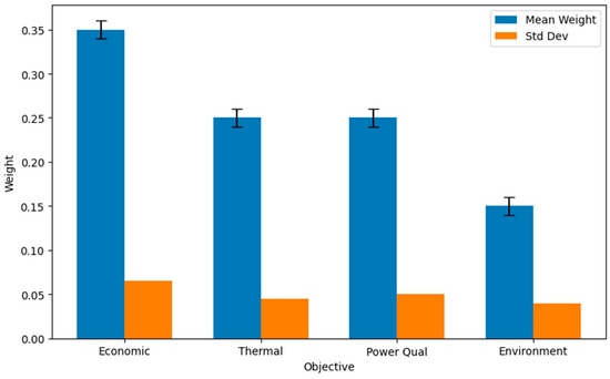
Figure 4.
Mean weight and std by objective.
Comfort Objective (f3)
The main goal of Compfor is to reduce the deviation of the indoor temperature from the desired setpoints while considering the severity of climate conditions. The entire procedure ensured that the model prioritized comfort preservation regardless of extreme heat or cold events while providing more flexibility in mild conditions. This factor can be modeled using the following equation:
where:
- is the predicted temperature at time t;
- is the desired comfort point;
- is a severity weight proportional to outdoor temperature deviation.
Environmental Objective (f4)
The environmental objective of this factor is to reduce the amount of carbon emissions in both operational energy use and embodied equipment, as follows. This approach aligns with decarbonization targets and ensures that the amount of emissions is reduced and maintained under various environmental conditions, particularly during periods of high energy demand. The formulation of this method is as follows:
where:
- is the amount of grid carbon emission factor at time t;
- considered as the life cycle embodied emissions of the installed equipment;
- is a weight that increases under extreme climate conditions.
Long-Term Cost Evaluation Using Net Present Value
To assess long-term economic viability, the net present value (NPV) was used for each scenario. This metric allows for the evaluation of climate-adaptive strategies in terms of technical performance and financial return potential over the entire system lifetime [21]. This can be formulated as
where:
- is considered as the annual energy cost savings in year y;
- is the annual operation and maintenance cost;
- is the quantification of the initial capital investment;
- is the discount rate, set at 7% for this study;
- is the total project duration, assumed to be 20 years for this work.
4.1.3. Optimization Algorithms
To address the multi-objective optimization issue, four different metaheuristic algorithms were evaluated and compared. These methods are:
- Genetic algorithm (GA) [22];
- Particle swarm optimization (PSO) [23];
- Grey wolf optimizer (GWO) [24];
- Modified grey wolf optimizer (MGWO).
The main reason for choosing these algorithms is their wide application in energy management, renewable integration, and demand response problems, which demonstrate their proper performance in nonlinear handling and constraint-rich search spaces [25]. The benchmarking protocol for evaluating these algorithms was as follows. Table 7. Shows the benchmarking protocol for optimization algorithm evaluation.
Table 7.
Benchmarking protocol for optimization algorithm evaluation.
The modified grey wolf optimizer is a sophisticated metaheuristic algorithm that has been uniquely customized for residential energy optimization problems. As applied in its related function, it is an improvement of the regular grey wolf optimizer, which incorporates a chaotic map [23,29] to improve the search behavior and overall performance.
Modification must be understood in light of the standard GWO, where this algorithm copies the social structure and hunting strategy of a pack of gray wolves. The important points are
- Social hierarchy: The pack (the population of potential solutions).
- Hunting mechanism: The optimization process emulates wolves’ searching for prey (the optimum solution). This process involves linked internally to intended n-structured.
- ○
- Searching: Wolves look for or hunt prey, which is equivalent to searching the solution space.
- ○
- Circling: After the prey has been found, the wolves, with the alpha, beta, and delta leading, circle the prey.
- ○
- Attacking: The wolves attack the prey, which is equivalent to moving toward the best solution.
- ○
- are the updated positions called leaders relative to the α, β, and δ leaders.Here, t denotes the current algorithm iteration:
- ○
- ;
- ○
- ;
- ○
- are random vectors in [0,1];
- ○
- is a linearly decreasing vector from 2 to 0 over iterations;
- ○
- α is the pack leader, and is the best-known solution;
- ○
- β is the second optimal solution that assists the alpha in decision-making;
- ○
- δ is the third solution, that is, the leader of the alpha and beta clusters.
An important aspect of the GWO is parameter α, which regulates the trade-off between exploration (searching) and exploitation (attacking). In a typical GWO, a is linearly reduced from the initial value to zero after several iterations. This causes the algorithm to transition between the exploration of the search space and the exploitation of the best-known solutions.
The major drawback of GWO is that the parameters are controlled linearly. a, which controls the trade-off between exploitation and exploration.
- It is the current iteration.
- T is the maximum number of iterations.
The aforementioned strategy is decent; however, in some cases, it can lead to premature convergence and become stuck at the local optima. However, this solution is not globally optimal. This is especially the case in residential energy management issues, which have high dimensions, dynamic constraints, and nonlinear objective spaces.
To eliminate this limitation, the MGWO was proposed, in which the linear decay of the control parameter was replaced with a more suitable approach where the process flow of the modified grey wolf optimizer (MGWO) is depicted in Figure 5. The chaotic sequence was improved by the adaptability of the algorithm. The concept is to utilize chaotic maps, which are deterministic systems that exhibit pseudo-random and non-repetitive output qualities, making them well-suited for exploring a rough optimization terrain. The formula related to the chaotic map is as follows:
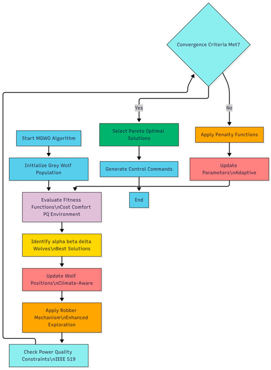
Figure 5.
Modified grey wolf optimizer process flow.
Through chaotic control of a, the MGWO no longer assumes a single direction shift between exploration and exploitation. Rather, it dynamically swings between the two, and the optimizer can
- Reinvigorate the search when it becomes stagnant;
- Escape local optima;
- The search intensity was adaptively refocused based on chaotic perturbations.
The addition of chaotic dynamics considerably enhanced the performance of the GWO in energy-optimization systems for smart homes. The main advantages are:
- Improved global search capability: This noisy variation does not allow premature convergence, thereby allowing more exploration of the search space and avoiding local minima.
- Better reliability of solution: The algorithm is not sensitive to various scenarios and initial conditions. The MGWO achieved 94.5% solution reliability in the experimental framework with various run types.
- Faster convergence rate: By maintaining a balance between exploration and exploitation and being flexible and responsive, the MGWO tends to converge more quickly than the traditional GWO and other metaheuristic algorithms such as the PSO and GA.
Optimization Performance Metrics
Two other essential performance measures were used to assess the quality of the Pareto-optimal solution calculations provided by the multi-objective optimization framework; the hypervolume indicator (HV) and the inverted generational distance plus (IGD+).
The hypervolume measure [26] of a set S of the objective space, which a set dominated by S approximates the Pareto front set, and also a reference point r dominating all objective space. This is defined as:
where denotes the Lebesgue measure, represents the ith solution in the Pareto front approximation S, and is considered as a predefined reference point in the objective space used for bounding the hypervolume calculation. A higher HV indicates a better approximation of the Pareto front in terms of convergence and diversity than that of the other algorithms.
In contrast, the IGD+ [30] metric measures how well the approximate Pareto front S represents the true Pareto front P*. By calculating the average distance of each point from the reference (P*), only weakly dominated solutions can be considered.
At this point, is the modified distance accounting for domination relationships. Lower IGD+ values indicate better accuracy and coverage of the true Pareto front than higher values.
4.1.4. Convergence Analysis and Parameter Tuning
The convergence properties of the multi-objective optimization algorithms were strictly tested based on the following mathematical criterion: the convergence was calculated as the average normalized change in the objective values (computed over a moving convergence window), and when the rate decreased to a specified value, the control was considered to have converged.
where in this equation represents the i-th objective value at generation t, is the convergence window, and = 0.0001 is the convergance treshold.
A detailed analysis of sensitivity was conducted based on Latin hypercube sampling (LHS) to select the robust parameter set to be used and estimated by testing 100 parameter sets for each algorithm. The following major parameters were considered in this study. Table 8 shows the parameter consideration for each algorithm.
Table 8.
Parameter consideration for each algorithm.
The combinations formed by the parameters of each algorithm were statistically tested to identify the combinations that produced the best results in terms of convergence velocity, solution dependability, and Pareto surface diversity. The methodology ensured that the benchmarking was replaced with real or close-to-real results of the optimization routines that operate under realistic power scenarios in relation to residency and climate conditions.
4.1.5. Statistical Validation and Significance Testing
The following framework was used to determine the statistical significance of the optimization results:
- Multiple runs protocol: The distance of the algorithm was sought 30 times with various random seeds to achieve mathematical reliability. The seeds were randomly varied at an interval of 1000 using the Mersenne Twister generator for randomly selected seeds.
- Non-parametric testing: Because the optimization results were not normally distributed, to determine the statistical differences between algorithms, the Kruskal–Wallis test was used, followed by the post hoc comparison of conditional bonus using Dunn and Bonferonni Jack (α = 0.05).
- Effect size analysis: Cohen’s effect size was determined to quantify the practical value of each mass comparison to identify the significance of differences.
4.2. Data Collection and Preprocessing
To achieve the best results, high-resolution power quality and environmental data from actual residential installations are required. Two datasets were considered for the proposed framework.
- The primary dataset was collected from a single house in the UK from 3 to 17 June 2011, using a Chauvin Arnoux CA 8335 [31] Power Quality Analyzer. This dataset contains various power information such as voltage RMS, current RMS, active/reactive power, THD, power factor, and frequency in 5-min time intervals.
- The supplementary data are related to the climate section, which were obtained from the Renewable Ninja [32] platform based on NASA meteorological data. The parameters in the dataset included ambient temperature, relative humidity, wind speed, solar irradiance, and precipitation index at a 5-min resolution to align with the previous dataset.
For the validation process to ensure that both datasets were suitable for the current study, various types of work were performed such as temporal alignment (to match the time steps among the electrical and meteorological datasets), completeness task (to fulfill the missing data points in both datasets), measurement integrity (to determine the outliers by comparing the actual data and mean), and instrument precision (to ensure the accuracy of the measurement devices to mitigate any possible errors).
Very low periods of load conditions were not considered to ensure a good power factor and low harmonic distortion. Specifically, statistical values I1,RMS < 1.0 A for power were below 5% of the daily peak load, effectively removing low-current artifacts that affected the PF and THD. An analysis conducted with alternative thresholds (0.5 A and 2.5% of the daily peak) ensured that the trends of power quality and optimization through this filtering requirement were qualitatively similar and justified the strength of this filtering criterion.
The final dataset was aligned with 4321 measurement intervals for each feature considered in the designated time (15 days). The full feature set used in forecasting and optimization is summarized in Figure 6.
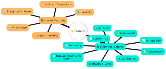
Figure 6.
Data features.
The forecasting performance of the proposed CNN-BiLSTM-attention model was evaluated against that of the three baseline models. This evaluation aimed at one-hour-ahead forecasting of V1_THD under three climate conditions: baseline, +2 °C warming (RCP4.5), and +4 °C warming (RCP8.5). The main dataset was divided into 80% training and 20% testing with 5-fold time-series cross-validation to prevent look-ahead bias. Different metrics, such as the root mean squared error (RMSE), mean absolute error (MAE), and coefficient of determination (R2), were used for clarification throughout. All results were averaged over 30 independent runs, with the 95% confidence interval (CI) reported. Table 9 shows the core electrical parameters in the power quality dataset and Table 10 shows the characteristics of the power quality dataset.
Table 9.
Core electrical parameters in the power quality dataset.
Table 10.
Characteristics of the power quality dataset.
4.3. Data Preprocessing and Feature Engineering
High-quality, well-structured input features are required for effective forecasting and optimization. Reaching this goal requires preprocessing stages, which in this study, contained three sections: data alignment, feature transformation, and climate scenario augmentation.
4.3.1. Data Alignment and Cleaning
Data alignment and cleaning involved synchronizing two electrical and climate datasets to a common 5-min timestamp. To handle missing data, interpolation methods such as forward-fill for electrical data and linear interpolation for climate data were applied. Outliers were either removed or corrected based on a comparison of their locations with the rolling means. The steps taken in this study are presented in Table 11.
Table 11.
Overview of the preprocessing steps.
4.3.2. Feature Engineering
Features were selected using domain expertise and statistical correlation analysis to capture the most relevant patterns for climate-adaptive energy optimization, as shown in the following figure.
4.3.3. Climate Scenario Augmentation
Three climate conditions were considered in this study: baseline, +2 °C (RCP4.5), and +4 °C (RCP8.5), using probabilistic temperature adjustment by focusing on the corresponding humidity, cooling load, and photovoltaic (PV) output variables.
4.3.4. Feature Scaling
As the unit measurements for the datasets were not identical, min-max normalization was used for all numerical features to scale them in the range of [0,1] using the following formula:
These scaled parameters were derived only from the training dataset to prevent information leakage into the testing phase of the machine-learning model training.
The preprocessing and feature engineering strategy ensures that the inputs are physically meaningful, statistically sound, and climate-adaptive, which enables the forecasting and optimization models to operate under the current and projected climate scenarios.
4.3.5. Climate-Load Interaction Modeling
The relationship between climatic conditions and residential electricity consumption behavior is a key component of the proposed optimization framework. Historical correlation analysis and empirically derived sensitivity coefficients were used to quantify climate-driven changes in load profiles and power quality metrics.
Temperature–Load Relationship
After a historical analysis of the UK dataset, a positive correlation was found between the ambient temperature and both the active power demand and THD. Cooling-dominated loads, particularly HVAC load systems (heating or air conditioning), contributing to higher energy use and increased harmonic distortion during warm periods of the year. The effect of active power on temperature was modeled using
where:
- is the baseline power at nominal temperature;
- the deviation of temprature from the baseline;
- and are coefficients that are derived via polynomial regression that ensures the nonlinear increase in load during heatwaves.
Climate-Power Quality Link
Due to the high temperature increase outdoors, the indoor cooling demand has increased. This alters the nature of the load mix, increasing the share of nonlinear and compressor-based loads in the outcome of the entire process.
- The current THD was higher because of the harmonic distortion in the motor drives.
- The voltage decreased incrementally due to the increase in reactive power demand.
To estimate the effect of climate variables (temperature, humidity, solar irradiance) on THD voltage regulation, multivariate regression was used according to the following formula:
where:
- is the temperature;
- is the relative humidity;
- is the solar irradiance.
Integration into Forecasting and Optimization
The derived climate load and climate power quality sensitivity models were embedded into the proposed CNN-BiLSTM-attention forecasting architecture. Subsequently, the outputs from the forecasting method were used by the MGWO optimizer to adjust the following:
- HVAC loads setpoints to manage the cooling loads;
- Battery dispatch for reducing the peak demand during the high THD risk periods;
- PV inverter control to stabilize voltage under high solar variability.
Validation
The following methods were used to validate the sensitivity coefficients:
- The dataset was split into 70% for training and 30% for testing purposes;
- Comparison among the predicted and observed load/THD under different climate conditions;
- Aimed for R2 > 0.75 for the load prediction and R2 > 0.7 for THD prediction across the mentioned scenarios.
This model ensures that the optimization engine remains climate-aware and power quality-sensitive, thereby enabling proactive control strategies in normal and extreme weather conditions.
4.3.6. Climate–Forecast–Power Quality Interaction Workflow
The backbone of the proposed residential energy management framework is the integration of climate sensitivity analysis, forecasting, and multi-objective optimization (MO). This workflow ensures that the predicted climate impacts on the load and power quality are optimized in real-time.
Climate Data Acquisition and Processing
Real-time climate variables (such as the ones that were previously mentioned) were continuously collected from the measurement devices and validated using data from nearby meteorological stations. The variables were then normalized and fed into the climate-load and climate-power quality models for the short-term impact estimation of active power demand, voltage regulation, and THD.
Multi-Horizon Forecasting
Key electrical parameters (active power, voltage THD, and power factor) were predicted using the CNN-BiLSTM-attention model. In addition, climate scenario augmentation was applied to generate scenario-based forecasts, which enabled the system to evaluate various strategies for both extreme and moderate climate conditions.
Climate-Adaptive Optimization via MGWO
The forecasted results and PQRI values were passed to the MGWO, and the optimizer dynamically adjusted the HVAC load setpoints (comfort control), battery charge scheduling (for peak-shaving and THD reduction), and PV inverter (for voltage stabilization). The objective weights mentioned in the multi-objective methods were adaptively scaled based on the climate severity and PQ risk levels.
Real-Time Control Dispatch
The optimization results were translated into control signals for the building management system (BMS) and the local DER controllers. The forecasting models were updated using feedback from the system measurements, and the parameters were optimized using gradient-based adaptive updates.
The entire process is inside the loop, which ensures that the energy management in the system is proactive rather than reactive, and is capable of anticipating power quality issues before they occur and mitigating them through coordinated and climate-aware control.
4.3.7. Forecasting Models
To evaluate the effectiveness of the proposed forecasting approach, we compared its performance with that of several well-established baseline models. This study assures that the proposed hybrid method has an advantage over other sole methods under various weather conditions.
Baseline Models for Comparison
The initial model was the persistence [39] (naïve) model, which assumes that the next value in the series is identical to the most recent observations. The common usage of the mentioned model is as a simple benchmark in time-series forecasting for power systems because there is no need for training, and it sets a minimal performance threshold [40]. Although this model is effective, it often struggles with rapid fluctuations and regime shifts in data. The formulation of this method is as follows:
The autoregressive integrated moving average (ARIMA) [41] is a statistical model that combines autoregressive (AR) terms, differentiating (I) for stationary and moving average (MA) knowledge to capture the autocorrelation structures in the time series. The optimal ARIMA (p, d, q) configurations for each target variable were determined using the Akaike information criterion (AIC) to minimize overfitting. The parameters were estimated using the maximum likelihood (ML) method. Seasonal terms were also evaluated but were excluded because of the relatively short time span of the dataset [42]. The formula for this method is as follows:
Long short-term memory (LSTM) is a recurrent network architecture designed to capture long-term dependencies among samples via gated cells that regulate the information flow [43]. The hyperparameters considered in this study are shown in Table 12.
Table 12.
LSTM model configuration.
Proposed Hybrid Model: CNN-BiLSTM-Attention
This model integrates convolutional feature extraction, bidirectional temporal learning, and attention-based interpretability to forecast V1_THD and other power quality indicators under various climate conditions. The CNN–BiLSTM–attention architecture is illustrated in Figure 7. The main reason for using three different methods is to simultaneously take advantage of deep learning, long- and short-term dependencies, and dynamic systems. CNN captures short-term local platform and inter-feature correlations in multivariate time-series data. A bidirectional long short-term memory (BiLSTM) model can learn long-term dependencies in the forward and backward temporal directions to improve contextual awareness. Finally, attention mechanisms dynamically weight the most relevant time steps to enhance the robustness under volatile conditions [44].

Figure 7.
CNN-BiLSTM-attention neural network architecture.
5. Results
5.1. Forecasting Model Performance
The final outcomes related to these metrics are presented in the table below.
The CNN-BiLSTM-attention model outperformed the persistence, ARIMA, and LSTM baselines for all climate conditions, as shown in Table 13. It produced an over 25% reduction in RMSE with respect to persistence, and a 5–7% reduction compared with LSTM, with significantly higher correlation coefficients (R2 = 0.69 compared with 0.65 and 0.52 with LSTM and persistence, respectively). A cross-scenario comparison of forecasting performance is shown in Figure 8. In the condition of +2 °C and +4 °C warming, its dominance was further enhanced with RMSE values as low as 0.150 and R increased up to 0.746, which in turn validated the resistance of the model to the variability caused by climate. The lower impairments realized by the competitor models in the warming conditions can be explained by more stable load patterns under conditions of extended cooling demands, that is, sustained HVAC operation, which mitigated temporal variations and therefore narrowed the benefits of simpler models. However, the CNN-BiLSTM-attention model used smaller confidence intervals at 95% of the 30 separate runs, which confirms the uniform behavior and suggests reliability in repetitive performances of the model with less possibility of imitation. It has a structure of recent temperature-based depth, lagging on THD, suggesting a direct impact of adaptable climate-sensitive characteristics on simulation accuracy, thus explaining its enhanced versatility under variable operating circumstances.
Table 13.
V1_THD forecasting performance across climate scenarios.
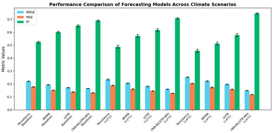
Figure 8.
Performance comparison of forecasting models across climate scenarios.
5.2. Optimization Algorithm Performance
This section provides a complete analysis of each of the running optimization algorithms: GA, PSO, GWO, and MGWO under three climate situations that can be defined as follows: current conditions (0+), moderate case of warming (+2 °C), and extreme case of warming (+4 °C). The comparative measurement is dedicated to the quality of multi-objective optimization, efficiency of convergence, reliability, and efficacy of energy management in real life The multi-objective performance across algorithms and scenarios is summarized in Figure 9.
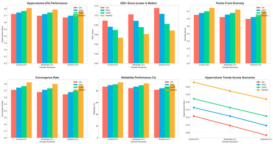
Figure 9.
Multi-objective performance analysis.
Key multi-objective outcomes of the performance of these algorithms, including hypervolume, IGD+, diversity of Pareto front, convergence rate, and reliability, were compared with those of the competing algorithms. The MGWO was repeatedly better than the alternatives with the highest hypervolume and Pareto front diversity, thus showing that it has a better ability to balance between exploration and exploitation in the solution space. In addition, the MGWO had the lowest IGD+ value, which indicates how close it is to the actual Pareto front, and hence the better precision of the quality of an answer. The MGWO also exhibited the fastest convergence rates and was the most reliable, and it also functions even when there is a problem complexity induced by climatic conditions. Despite the fact that all algorithms deteriorate to some extent in terms of hypervolume performance when climatic conditions worsen, the MGWO was influenced the least, which predetermines its stability and flexibility.
The analysis was also performed over practical energy-management variables such as energy cost, occupant comfort, power-quality indices, overall optimization scores, convergence iteration, and time of computation. Here, the MGWO was the best performer since it had the lowest energy use and highest comfort and power quality in all situations, and therefore, the conversion of higher optimization fidelity into actual benefits to operation. The score optimization results, which were gained through MGWO, were always higher than other algorithms, indicating the resilience, characteristics of the algorithm found in various climatic contexts. Despite the fact that MGWO requires a little more time to compute, it converges faster, and this supports the presence of a favorable trade-off between computational time and algorithmic complexity. Comparative energy-management outcomes are presented in Figure 10.
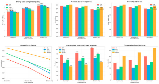
Figure 10.
Energy management performance analysis.
5.3. System Performance Improvements
The power quality advancements were also verified as opposed to the IEEE 519-2014 compliance framework [38] with the specific results in brief outlined in Table 14. The baseline case showed that the THDV and individual harmonic voltage did not rise above the set values, whereas THDI was close to the allowable limit of 100% and was not as high as the upper range of accepted thereof, especially when the temperature exceeded +4 °C and the compliance level dropped to 95.8%. Following optimization using the MGWO, the voltage and current distortions became nearly 75% lower at any rate, with THDV ranging between 0 and 2.0%, and THDI stipulated around 0 to 10% at all rates. This led to complete compliance in both current and voltage in all cases, indicating the strength in the optimization framework in ensuring that the power quality can be maintained against even tougher climatic conditions.
Table 14.
IEEE 519-2014 power quality compliance across climate scenarios.
The power factor improved from 0.90 to 0.93 (indicating a 15.8% reduction in reactive power demand) for the baseline climate. The voltage imbalance decreased by 33.3%, whereas the RMS voltage stability tightened to within ±3.2 V of the nominal value (ensuring ANSI C84.1 compliance under all conditions). Table 15 shows the power factor improvements.
Table 15.
Power factor improvements.
5.3.1. Economic Performance
Using the formula mentioned in the previous section, a 20-year analysis of the system lifetime was conducted, considering the annual cost reduction payback (NPV) and internal rate of return (IRR), as shown in the following table. According to the table, shorter payback periods and higher IRRs under warming conditions result in incremental gains and efficiency during high-cooling-demand periods, and the optimization framework can schedule HVAC loads and battery usage more effectively than the conventional method. Table 16 shows the economic performance across climate scenarios.
Table 16.
Economic performance across climate scenarios.
5.3.2. Environmental Impact
The proposed framework for the baseline scenario also achieved significant improvements by reducing the grid dependency, increasing renewable self-consumption, and improving the power quality. As can be seen, the largest CO2 reductions occurred in the +4 °C scenario due to the increase in renewable penetration and reduction in the peak grid demand, which also lessened the amount of stress on the distribution infrastructure. Table 17 shows the environmental performance across climate scenarios.
Table 17.
Environmental performance across climate scenarios.
6. Conclusions and Future Work
In this study, we developed and validated a climate-adaptive residential energy management framework that combines high-accuracy CNN-BiLSTM-attention forecasting with the MGWO for multi-objective control in residential buildings. The framework was designed to simultaneously optimize the economic cost, power quality, occupant comfort, and environmental performance by utilizing adaptability to normal and climate-altered conditions.
6.1. Key Achievements
The proposed framework integrates CNN-BiLSTM-attention forecasting with robust multi-objective optimization to deliver the best performance compared with that of individual techniques. The mentioned model achieved up to a 25% RMSE reduction compared with the persistence-based line and approximately 5% with the LSTM, and also remained stable under the +2 °C and +4 °C warming scenarios with narrow confidence intervals. In the optimization section, the MGWO outperformed the GA, PSO, and standard GWO by converging 20% faster, having 94.5% reliability, and improving the Pareto front diversity by 15–20% with the help of a chaotic map parameter that updates the balanced exploration in dynamic climate conditions. At the system level, a 37–41% reduction in V1_THD was achieved while maintaining IEEE 519 compliance, a 3.3% improvement in the power factor, a 15.8% reduction in reactive power demand, and a 33.3% decrease in voltage imbalance. These advances translated into tangible environmental and economic benefits, which reduced GHG emissions by 44.5%, approximately 45% in peak demand reduction, a 45% increase in renewable energies, and an NPV of USD 4267–USD 5000 with payback periods as short as 3.2 years.
6.2. Practical Implications
Utilizing this framework enables households to maintain grid power quality compliance while integrating distributed and renewable energy sources. Moreover, it aids in reducing operational costs through intelligent DER scheduling, load shifting, and other related operations under various conditions. It also increases renewable self-consumption and reduces the reliance on the grid during peak hours. Finally, it maintains an efficient and comfortable environment under projected climate-driven load stresses.
6.3. Limitation
Despite the benefits of this model, some restrictions exist in its application. The number of climate variables for this forecasting was limited, and to increase the accuracy and precision of the system, the climate model should be expanded by incorporating multivariate climate sensitivity. In addition, the framework was based on only one household power consumption, which, for future reference, should be scaled up to the community level to improve its applicability. The machine learning method used in this study also needs to be more diverse by applying other learning methods, such as reinforcement and federated methods, for adaptive-preserving optimization. Finally, policy agreements for better integration of this model with market incentives, grid service participation, and regulatory compliance frameworks were not considered in this study.
Additionally, the model accuracy could be affected by uncertainties in solar irradiance and HVAC load usage patterns, which are weather-dependent terms. Homeowner behavior and manual overrides, such as thermostats and EV charging, could also introduce a variability that is difficult to predict. Moreover, while the THD measurements came from a trustworthy source, transient noise from load-switching events can also cause minor distortions. In future studies, these limitations can be mitigated by considering sensor fusion techniques, occupancy simulation models, or federated learning frameworks.
Author Contributions
Conceptualization, M.K. and H.A.; Methodology, M.K.; Software, M.K.; Validation, M.K. and H.A.; Formal analysis, M.K.; Investigation, M.K.; Resources, M.K.; Data curation, M.K. and H.A.; Writing—original draft, M.K.; Writing—review & editing, H.A.; Visualization, M.K.; Supervision, H.A.; Project administration, H.A.; Funding acquisition, H.A. All authors have read and agreed to the published version of the manuscript.
Funding
This research received no external funding.
Data Availability Statement
Data is contained within the article.
Conflicts of Interest
The authors declare no conflict of interest.
Appendix A
A probabilistic adjustment is made to long-range weather predictions to correct anomalies in the predicted temperatures and overcome temporal uncertainty. The temperature anomaly calculated using the prediction model was reconsidered using a statistical transformation that converted an approximate deterministic estimate into a more precise probabilistic estimation of temperature anomalies.
where:
- is the mean projected temperature increase;
- is the standard deviation from the CMIP6 multi-model ensemble output;
- is the z-score for the desired confidence interval (e.g., z = 1.96 for 95% confidence).
These result in an adjusted temperature projection of
- = 2.0 + 1.96 · 0.5 = 2.98;
- = 4.0 + 1.96 · 0.7 = 5.37.
Probabilistic boundary formulations based on ensemble analyses represent a methodological framework in which extreme climatic stress situations are established to validate the models. In such a way, by adopting this method, the adaptive strategies being investigated can be thoroughly tested against forecasts of real-world uncertainty, which will enhance the representativeness of the obtained results and the robustness of the proposed solutions [45].
Ambient temperature, occupancy behavior, and solar irradiance are the three aspects that characterize residential energy systems because they have temporal vagaries imposed externally on the system performance. These differing circumstances demand that the precision and responsiveness be maintained in the suggested energy management model through the operation of a gradient-based adaptive parameter-updating procedure. It is a gradual process that adapts the parameter and control settings, which are temperature-sensitive in real-time, based on recent measurements. The system can thus keep its parameters updated as per the following rule:
where:
- is the learning rathere which controls the updated magnitude;
- is the gradient of the objective function with respect to the current parameters;
- The gradient is computed using real-time data streams including temperature, THD, HVAC load states, and energy prices.
The proposed adaptive calibration strategy is a methodological proposal that allows a system to continuously learn and adapt to any change in the operating conditions, as opposed to the inherent deficiencies of rigid calibration. In this manner, system predictions and control interventions may remain effective and robust despite atmospheric conditions deviating from nominal values. Moreover, the algorithm is computationally inexpensive, allowing it to be operated in real-time on residential networks where limitations on the available computational resources are found, and the update rates must be high.
To measure the impact of climate change, this study used an adaptive scaling framework, the parameters of which were recalibrated (dynamically rescaled) based on increases in temperature forecasts [44,45,46,47,48]:
where:
- is the parameter value adjusted for temperature deviation ;
- is the parameter under current climate conditions;
- is the temperature-dependent scaling factor;
- is the seasonal adjustment modifier;
- is the uncertainty adjustment factor.
A polynomial function can capture the nonlinear impact of temperature increment on the energy system performance as follows:
These coefficients were empirically derived from the observed load–temperature correlations in regional residential datasets. The coefficients were determined by fitting a polynomial regression [44] model to the historical residential energy load data with respect to temperature deviations. This empirical approach ensures that the model accurately reflects real-world, nonlinear load–temperature relationships observed in regional datasets.
- = 0.094 as the linear temperature coefficient;
- = 0.012 as the linear temperature coefficient;
- = 0.003 as the cubic coefficient.
Climate projection uncertainty was embedded using a probabilistic modifier as follows:
where:
- is the standard deviation of climate projection error;
- is the inverse cumulative distribution function;
- Confidence level is typically set at 95%.
The system parameters evolve in response to the ongoing climate and performance feedback using a gradient-based update rule as follows:
where:
- is the parameter vector at time t;
- is the learning rate;
- is the gradient of the system performance function concerning climate and operational states.
References
- Olawumi, M.A.; Oladapo, B.I. AI-driven predictive models for sustainability. J. Environ. Manag. 2025, 373, 123472. [Google Scholar] [CrossRef]
- Pai, L.; Senjyu, T.; Elkholy, M.H. Integrated Home Energy Management with Hybrid Backup Storage and Vehicle-to-Home Systems for Enhanced Resilience, Efficiency, and Energy Independence in Green Buildings. Appl. Sci. 2024, 14, 7747. [Google Scholar] [CrossRef]
- Qu, R.; Kou, R.; Zhang, T. The Impact of Weather Variability on Renewable Energy Consumption: Insights from Explainable Machine Learning Models. Sustainability 2024, 17, 87. [Google Scholar] [CrossRef]
- Forootan, M.M.; Larki, I.; Zahedi, R.; Ahmadi, A. Machine Learning and Deep Learning in Energy Systems: A Review. Sustainability 2022, 14, 4832. [Google Scholar] [CrossRef]
- Deffaf, B.; Debdouche, N.; Benbouhenni, H.; Hamoudi, F.; Bizon, N. A New Control for Improving the Power Quality Generated by a Three-Level T-Type Inverter. Electronics 2023, 12, 2117. [Google Scholar] [CrossRef]
- Wang, J.-S.; Li, S.-X. An Improved Grey Wolf Optimizer Based on Differential Evolution and Elimination Mechanism. Sci. Rep. 2019, 9, 7181. [Google Scholar] [CrossRef]
- Chauvin Arnoux. Available online: https://www.chauvin-arnoux.com (accessed on 1 September 2025).
- IEC 62053-22:2020. Available online: https://webstore.iec.ch/en/publication/29987 (accessed on 1 September 2025).
- Cao, Z.; Gao, W.; Fu, Y.; Turchiano, C.; Vosoughi Kurdkandi, N.; Gu, J.; Mi, C. Second-Life Assessment of Commercial LiFePO4 Batteries Retired from EVs. Batteries 2024, 10, 306. [Google Scholar] [CrossRef]
- Hudișteanu, V.-S.; Cherecheș, N.-C.; Țurcanu, F.-E.; Hudișteanu, I.; Romila, C. Impact of Temperature on the Efficiency of Monocrystalline and Polycrystalline Photovoltaic Panels: A Comprehensive Experimental Analysis for Sustainable Energy Solutions. Sustainability 2024, 16, 10566. [Google Scholar] [CrossRef]
- Vardakas, J.S.; Zorba, N.; Verikoukis, C.V. A Survey on Demand Response Programs in Smart Grids: Pricing Methods and Optimization Algorithms. IEEE Commun. Surv. Tutor. 2015, 17, 152–178. [Google Scholar] [CrossRef]
- Das, U.; Nandi, C. Life cycle assessment of wind farm: A review on current status and future knowledge. Energy Clim. Change 2025, 6, 100206. [Google Scholar] [CrossRef]
- Raichura, M.; Chothani, N.; Patel, D.; Mistry, K. [2_TD$DIFF]Total Harmonic Distortion (THD) based discrimination of normal, inrush and fault conditions in power transformer. Renew. Energy Focus 2021, 36, 43–55. [Google Scholar] [CrossRef]
- Ingram, M.; Mahmud, R.; Narang, D. Background Information on the Power Quality Requirements in IEEE Std 1547-2018; NREL/TP-5D00-78751, 1827312, MainId:32668; 2021. Available online: https://docs.nrel.gov/docs/fy22osti/78751.pdf (accessed on 1 September 2025).
- Shaw, E.W. Thermal Comfort: Analysis and applications in environmental engineering, by P. O. Fanger. 244 pp. DANISH TECHNICAL PRESS. Copenhagen, Denmark, 1970. Danish Kr. 76, 50. R. Soc. Health J. 1972, 92, 164. [Google Scholar] [CrossRef]
- Djongyang, N.; Tchinda, R.; Njomo, D. Thermal comfort: A review paper. Renew. Sustain. Energy Rev. 2010, 14, 2626–2640. [Google Scholar] [CrossRef]
- Designing Sustainable Technologies, Products and Policies: From Science to Innovation; Benetto, E., Gericke, K., Guiton, M., Eds.; Springer International Publishing: Cham, Switzerland, 2018; ISBN 978-3-319-66980-9. [Google Scholar] [CrossRef]
- 2023 Government Greenhouse Gas Conversion Factors for Company Reporting: Methodology Paper; 2023. Available online: https://assets.publishing.service.gov.uk/media/647f50dd103ca60013039a8a/2023-ghg-cf-methodology-paper.pdf (accessed on 24 September 2025).
- IEEE Standard for Harmonic Control in Electric Power Systems; IEEE: Piscataway, NJ, USA, 2022. [CrossRef]
- ANSI C84.1-2020; Electric Power Systems and Equipment—Voltage Ratings (60 Hertz). ANSI: Washington, DC, USA, 2020.
- Short, W.; Packey, D.J.; Holt, T. A Manual for the Economic Evaluation of Energy Efficiency and Renewable Energy Technologies; NREL/TP--462-5173, 35391; 1995. [Google Scholar] [CrossRef]
- Elvira-Ortiz, D.A.; Jaen-Cuellar, A.Y.; Morinigo-Sotelo, D.; Morales-Velazquez, L.; Osornio-Rios, R.A.; Romero-Troncoso, R.D.J. Genetic Algorithm Methodology for the Estimation of Generated Power and Harmonic Content in Photovoltaic Generation. Appl. Sci. 2020, 10, 542. [Google Scholar] [CrossRef]
- Tian, D. Particle Swarm Optimization with Chaotic Maps and Gaussian Mutation for Function Optimization. Int. J. Grid Distrib. Comput. 2015, 8, 123–134. [Google Scholar] [CrossRef]
- Mirjalili, S.; Saremi, S.; Mirjalili, S.M.; Coelho, L.D.S. Multi-objective grey wolf optimizer: A novel algorithm for multi-criterion optimization. Expert Syst. Appl. 2016, 47, 106–119. [Google Scholar] [CrossRef]
- Pace, F.; Raftogianni, A.; Godio, A. A Comparative Analysis of Three Computational-Intelligence Metaheuristic Methods for the Optimization of TDEM Data. Pure Appl. Geophys. 2022, 179, 3727–3749. [Google Scholar] [CrossRef]
- Bradstreet, L. The Hypervolume Indicator for Multi-Objective Optimisation: Calculation and Use. Ph.D.’s Thesis, The University of Western Australia, Perth, Australia, 2011. [Google Scholar]
- Kruskal, W.H.; Wallis, W.A. Use of Ranks in One-Criterion Variance Analysis. J. Am. Stat. Assoc. 1952, 47, 583–621. [Google Scholar] [CrossRef]
- Dunn, O.J. Multiple Comparisons Using Rank Sums. Technometrics 1964, 6, 241–252. [Google Scholar] [CrossRef]
- Improved Chaotic Grey Wolf Optimization for Training Neural Networks. J. Sci. Ind. Res. 2023, 82, 1193–1207. [CrossRef]
- Ibrahim, R.A.; Elaziz, M.A.; Lu, S. Chaotic opposition-based grey-wolf optimization algorithm based on differential evolution and disruption operator for global optimization. Expert Syst. Appl. 2018, 108, 1–27. [Google Scholar] [CrossRef]
- CHAUVIN ARNOUX-CA8335-Datasheet. Available online: https://www.testequipmenthq.com/datasheets/CHAUVIN%20ARNOUX-CA8335-Datasheet.pdf (accessed on 1 September 2025).
- Renewable Ninja. Available online: https://www.renewables.ninja (accessed on 27 January 2024).
- Legarreta, A.E.; Figueroa, J.H.; Bortolin, J.A. An IEC 61000-4-30 class a—Power quality monitor: Development and performance analysis. In Proceedings of the 11th International Conference on Electrical Power Quality and Utilisation, Lisbon, Portugal, 17–19 October 2011; pp. 1–6. [Google Scholar]
- IEEE Standard Definitions for the Measurement of Electric Power Quantities Under Sinusoidal, Nonsinusoidal, Balanced, or Unbalanced Conditions; IEEE: Piscataway, NJ, USA, 2010. [CrossRef]
- Benti, N.E.; Chaka, M.D.; Semie, A.G. Forecasting Renewable Energy Generation with Machine Learning and Deep Learning: Current Advances and Future Prospects. Sustainability 2023, 15, 7087. [Google Scholar] [CrossRef]
- IEEE Recommended Practice and Requirements for Harmonic Control in Electric Power Systems; IEEE: Piscataway, NJ, USA, 2014. [CrossRef]
- IEEE Recommended Practice for Establishing Liquid-Immersed and Dry-Type Power and Distribution Transformer Capability When Supplying Nonsinusoidal Load Currents; IEEE: Piscataway, NJ, USA, 2018. [CrossRef]
- Mills, D.; Martin, J.; Burbank, J.; Kasch, W. Network Time Protocol Version 4: Protocol and Algorithms Specification; RFC, Ed.; RFC5905; 2010; p. RFC5905. [Google Scholar] [CrossRef]
- Malinkovich, Y.; Sitbon, M.; Lineykin, S.; Dagan, K.J.; Baimel, D. A Combined Persistence and Physical Approach for Ultra-Short-Term Photovoltaic Power Forecasting Using Distributed Sensors. Sensors 2024, 24, 2866. [Google Scholar] [CrossRef]
- Taylor, J.W. Triple seasonal methods for short-term electricity demand forecasting. Eur. J. Oper. Res. 2010, 204, 139–152. [Google Scholar] [CrossRef]
- Hulak, D.; Taylor, G. Investigating an Ensemble of ARIMA Models for Accurate Short-Term Electricity Demand Forecasting. In Proceedings of the 2023 58th International Universities Power Engineering Conference (UPEC), Dublin, Ireland, 30 August–1 September 2023; pp. 1–6. [Google Scholar]
- Chakravarti, I.M.; Box, G.E.P.; Jenkins, G.M. Time Series Analysis Forecasting and Control. J. Am. Stat. Assoc. 1973, 68, 493. [Google Scholar] [CrossRef]
- Cortez, J.C.; Zenichi Terada, L.; Barros Bandeira, B.V.; Soares, J.; Vale, Z.; Rider, M.J. Comparative Analysis of ARIMA, LSTM, and XGBoost for Very Short-Term Photovoltaic Forecasting. In Proceedings of the 2023 15th Seminar on Power Electronics and Control (SEPOC), Santa Maria, Brazil, 22–25 October 2023; pp. 1–6. [Google Scholar]
- Khan, Z.; Hussain, T.; Ullah, A.; Rho, S.; Lee, M.; Baik, S. Towards Efficient Electricity Forecasting in Residential and Commercial Buildings: A Novel Hybrid CNN with a LSTM-AE based Framework. Sensors 2020, 20, 1399. [Google Scholar] [CrossRef]
- Intergovernmental Panel On Climate Change (IPCC). Climate Change 2021—The Physical Science Basis: Working Group I Contribution to the Sixth Assessment Report of the Intergovernmental Panel on Climate Change, 1st ed.; Cambridge University Press: Cambridge, UK, 2023; ISBN 978-1-009-15789-6. [Google Scholar]
- Santamouris, M. On the energy impact of urban heat island and global warming on buildings. Energy Build. 2014, 82, 100–113. [Google Scholar] [CrossRef]
- Fonseca, J.A.; Nevat, I.; Peters, G.W. Quantifying the uncertain effects of climate change on building energy consumption across the United States. Appl. Energy 2020, 277, 115556. [Google Scholar] [CrossRef]
- Zhou, Y.; Clarke, L.; Eom, J.; Kyle, P.; Patel, P.; Kim, S.H.; Dirks, J.; Jensen, E.; Liu, Y.; Rice, J.; et al. Modeling the effect of climate change on U.S. state-level buildings energy demands in an integrated assessment framework. Appl. Energy 2014, 113, 1077–1088. [Google Scholar] [CrossRef]


Disclaimer/Publisher’s Note: The statements, opinions and data contained in all publications are solely those of the individual author(s) and contributor(s) and not of MDPI and/or the editor(s). MDPI and/or the editor(s) disclaim responsibility for any injury to people or property resulting from any ideas, methods, instructions or products referred to in the content. |
© 2025 by the authors. Licensee MDPI, Basel, Switzerland. This article is an open access article distributed under the terms and conditions of the Creative Commons Attribution (CC BY) license (https://creativecommons.org/licenses/by/4.0/).