Abstract
This paper presents a comprehensive study of parameter estimation for three-phase induction motors (IMs) using hybrid optimization methods and a comparative evaluation of static and dynamic modeling approaches. A hybrid metaheuristic combining the Sine Cosine Algorithm (SCA) and Particle Swarm Optimization (PSO) is developed to identify optimal motor parameters efficiently. The approach utilizes a static model for rapid estimation, with final parameter values validated against a dynamic model to ensure accuracy in operational predictions. Results confirm that the static model provides robust parameter estimates for key performance metrics, including torque, power factor, and current, aligning well with experimental results from real-motor no-load tests. Parameters estimated by the proposed method demonstrate a high adherence with the motor real measurements. Comparisons also reveal the limitations of static models in scenarios requiring state-space accuracy, such as observer-based control applications. This study concludes by recommending further exploration of alternative motor modeling structures and the hybrid optimization algorithm for parameter estimation.
1. Introduction
The identification of induction motor (IM) parameters has been extensively studied, with most approaches based on the per-phase static model of induction motors to determine machine parameters. Standards like IEEE 112 [1] and IEC 60034 [2] are pivotal in this area, offering reliable parameter references widely adopted in both academia and industry. Variations on these standard models are common in IM research, such as the double-cage model (DCM) [3,4] and models incorporating core and stray load loss resistors [5].
Despite their popularity, the static models and their variations are limited in handling transient states, restricting their effectiveness in control systems [6]. Consequently, essential control tools for three-phase induction motors—such as the Extended Kalman Filter (EKF), Unscented Kalman Filter (UKF), Model Predictive Current Control (MPCC), Direct Torque Control (DTC), and Model Reference Adaptive System (MRAS)—are instead built on the dynamic model [7,8].
The dynamic model, however, is significantly more complex. Its mechanical model couples with electromechanical nonlinear differential equations, increasing the system’s parameter count and overall complexity, which enhances adherence to real-world behaviors, enabling more accurate predictions in dynamic conditions.
Beyond these well-known differences, a practical distinction between static and dynamic models lies in their computational demand. In fact, static models enable near-instantaneous calculation of operational variables, while dynamic models necessitate iterative solutions of nonlinear equations, resulting in longer simulation times.
These theoretical and practical distinctions raise interesting questions: How different are the operational outputs calculated from both models? Does this difference require distinct parameter sets to accurately describe the same IM in each approach?
Related Works
An analysis of IM parameter estimation methods reveals that most rely on the static model, including the IEEE [1] and IEC [2] standards, which depend on this kind of model to make many conclusions concerning the motor power balance and the necessary measurements to determine motor operational parameters. Also, the traditional no-load and blocked-rotor tests described in [1] rely on the static model to determine the induction motor parameters. Despite its unquestionable success, some drawbacks make their use difficult in many situations, such as the change in the coupled load, the demand for specific measurements like power measurement, and the use of low-frequency sources [9]. To address these drawbacks, various studies propose alternative estimation methods.
In [3], a numerical method is presented to estimate double-cage model equivalent circuit parameters, based on five operational measurements. This method, however, does not account for core losses and requires significant effort to estimate the relationship between rotor leakage inductances. The results are validated through inverse calculation, which derives datasheet data from the estimated parameters, yielding low error values.
Similarly, ref. [4] develops a method using a double-cage model equivalent circuit, but relies on a nonlinear optimization procedure to find the model parameters. This method is applied to a single motor and validated through torque–speed curve alignment. Like the previous work, it also uses inverse calculation for validation, achieving an error below 5%
In [10], an analytical method is introduced, using operational data across various loads, as found in manufacturer datasheets. This method, based on the machine’s power balance and a single-cage model without core loss, yields low error across a range of motors. However, its assessment remains limited to inverse calculation, and while a case study is included, no practical measurements were conducted.
In another study, ref. [11] utilizes a genetic algorithm to estimate three induction motor parameters from datasheet information via a static model. Here, a heuristic imposing loss limitations is used to enhance accuracy. The results are then compared to catalog data and local measurements, but relatively high deviations are reported, attributed to the datasheet’s low accuracy and the absence of real tests.
The work in [12] takes a more complex approach, estimating 18 parameters for an induction motor dynamic model that includes iron losses and magnetic saturation, using a genetic algorithm to optimize parameter selection. Despite the model’s complexity, low error levels are achieved compared to measured values. This method, however, requires motor testing under various loads, which could limit its applicability where motors are already installed or load control is unavailable.
In another paper, ref. [13] employs a two-stage Particle Swarm Optimization (PSO) algorithm to estimate the parameters of single-cage induction motors (IMs) using manufacturer-provided data. The resulting torque–speed curve demonstrates good agreement with the manufacturer’s specifications. However, no practical measurements were conducted to validate these results. Similarly, ref. [14] presents an artificial neural network (ANN) approach for determining IM parameters, yielding outputs with negligible errors. Nevertheless, the source of the IM parameter dataset and the original method used to estimate these parameters remain unclear. Moreover, as with the previous study, no practical validation was performed.
Despite these contributions, to the best of our knowledge no paper deals with the differences and similarities between the static model and the dynamic model, nor even the different results that they can provide. This subject has a high relevance, as the final application of the estimated parameters should be considered to determine the estimation method. Regarding this relevant subject, an important question arises: can the parameters estimated by a static model be used in a dynamic model?
Aiming to investigate this issue, this study provides a detailed calculation of various operational parameters for induction motors using both static and dynamic models. Additionally, a novel Hybrid PSO-SCA Optimization Algorithm (HPSOA) is proposed to estimate the parameters of a real induction motor based on the static model. The parameters obtained from the static model are validated using the dynamic model, highlighting the strengths and weaknesses of this approach. To complement the simulations presented in this work, practical validation is also performed, ensuring the reliability of the results.
In Section 2, the static model utilized in this study is presented. Section 3 details the dynamic model and its fundamental equations. Section 4 explains the calculation of performance parameters commonly listed in datasheets using both models. Section 5 covers loss calculations. The optimization algorithm, metaheuristics, and hybrid solution validation are presented in Section 7. In Section 6, two sets of induction motor (IM) parameters are used to feed both dynamic and static motor models, allowing for a comparison of the differences between their outputs. Results and discussions are provided in Section 8 and Section 9, respectively, with conclusions summarized in Section 10.
2. Static Model
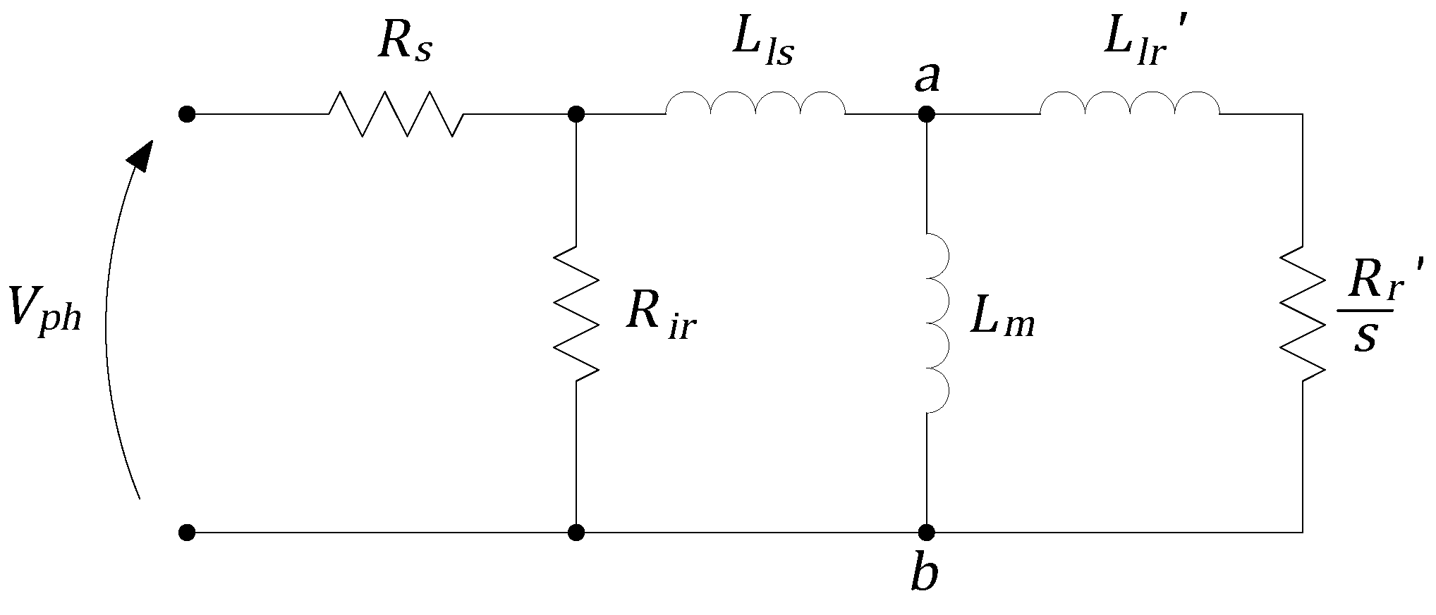
The induction motor (IM) static model represents the machine’s voltages and currents through a simplified electrical circuit. This model can predict many of the electric and mechanical quantities associated with machine operation with reasonable accuracy. Various configurations of this circuit are found in the literature, each with distinct features. The “single cage with core loss” configuration, depicted in Figure 1, is used in this work.
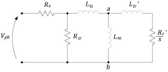
Figure 1.
Single cage with core loss equivalent circuit.
This equivalent circuit provides the most comprehensive static representation, as it includes three resistances that model typical types of losses in an induction machine: stator copper loss, rotor copper loss, and iron loss, represented by resistances , , and , respectively. The model does not account for the two additional significant losses—rotational loss and stray load loss—which should be considered externally. This exclusion is generally accepted for rotational losses.
The single cage with core loss model used in this work differs significantly from those defined by IEEE 112 and IEC 60634-2 standards [1,2]. Here, we base our approach on the circuit proposed in [15,16], where the leakage flux and magnetizing flux are combined. This adjustment simplifies the dynamic equations, making them easier to handle, as will be explained in the next section.
3. Dynamic Model
The dynamic model used in this work builds upon the equivalent circuit configuration introduced in the previous section. Here, the leakage inductance and magnetizing inductance of the stator and rotor are grouped, ensuring the same current flows through them. This arrangement simplifies the dynamic model representation while retaining fidelity to the real machine’s behavior.
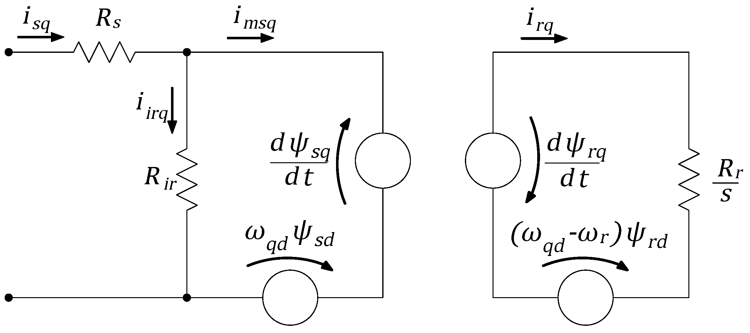
To provide a streamlined view of the circuit, the stator and rotor leakage and magnetizing inductances are grouped together. In Figure 2, the equivalent circuit for the q-axis components is shown. This representation introduces a coupling term in the stator and rotor as a consequence of the magnetic flux derivative, which is characteristic of qd machine representations. In this configuration, the coupling term appears close to the derivative term, preceding the node with resistance . The mathematical equations representing this model, initially developed in [15,16], are provided in Equations (1)–(14). Table 1 defines the variables used in these equations. All the voltages, currents, and magnetic fluxes listed in this table were projected in the synchronous reference frame for the dynamic simulations performed in this paper.
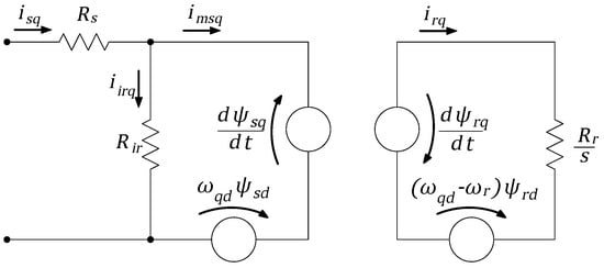
Figure 2.
Single cage with core loss equivalent circuit, illustrating magnetic coupling between stator and rotor.

Table 1.
IM equation variables mentioned in the text.
In this configuration, the magnetizing currents and differ from the input currents and . This relationship, derived from Kirchhoff’s Current Law (KCL), is detailed in Equations (5) and (6). Consequently, the equations for the rotor and stator direct and quadrature magnetic fluxes (, , , ) are not explicitly expressed as functions of the stator currents (or grid line currents) and , as shown in Equations (9)–(12). This complexity makes the iterative solution of the differential equations more challenging.
To overcome this issue, the variables and in Equations (1) and (2) can be replaced using the relationships provided in Equations (5) and (6). By applying this substitution and performing further mathematical manipulations, Equations (15) and (16) can be derived. These equations describe the time variation of fluxes and as functions of the magnetizing currents and and magnetic fluxes and .
Thevenin Equivalent Circuit
The calculation of some performance parameters of IMs is simplified when the Thevenin equivalent circuit is used. This procedure is similar to the procedure explained in most machine books, like [9,17]. The base circuit is already presented in Figure 1, where the a and b points delimit the equivalent circuit, composed by the stator resistance , iron resistance , stator inductance , and magnetizing inductance . Making the voltage source a short circuit, the equivalent circuit becomes the one shown in Figure 3.
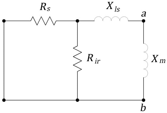
Figure 3.
Fragment of IM model used to calculate the Thevenin resistance, with the phase voltage source short-circuited.
4. Performance Parameters
The primary performance parameters used to analyze three-phase induction motors are typically available in manufacturer datasheets. These parameters are also covered in the electrical machine literature, where they are calculated based on the static model. In the following sections, the calculation of these parameters is outlined, with explicit distinctions between static and dynamic model approaches.
4.1. Torque Equations
In the dynamic model of an induction motor (IM), the instantaneous electromagnetic torque is derived from variations in the magnetic field stored in the machine inductances, excluding the leakage inductances. The mathematical development for this is detailed in [18], resulting in Equation (23).
To determine the instantaneous electromagnetic torque at different rotor speeds, the motor can be simulated to reach specific speed conditions, where torque values are then measured using Equation (23). Mechanical variables can be manipulated in the blocked rotor and no-load tests, with the blocked rotor test being the preferred method for capturing starting torque as it minimizes current transients associated with free acceleration.
In contrast, in the static model, the electromagnetic torque is derived from the power balance of the equivalent circuit, expressed as a function of slip, supply voltage, and motor parameters. As shown in [9,17], the Thevenin equivalent circuit is commonly used to simplify the torque equation. In this approach, the stator parameters and the magnetizing inductance are used to calculate the Thevenin voltage and the Thevenin impedance, represented by resistance and inductive reactance . The grid synchronous frequency is also incorporated and the final expression for steady-state electromagnetic torque is expressed in Equation (24).
4.1.1. Starting Torque
In the static model, starting torque is calculated from Equation (24) by setting the slip equal to 1, corresponding to a rotor speed of 0 RPM. The resulting expression is similar to Equation (24), as given in Equation (25):
As noted above, in the dynamic model, starting torque is obtained using the blocked rotor test.
4.1.2. Maximum Torque
In the static model, the maximum torque is determined from Equation (24) by first finding the slip s that satisfies . This is given in Equation (26).
In the dynamic model, maximum torque is obtained by identifying the peak torque observed during a free acceleration test.
4.2. Efficiency
Efficiency calculations differ between the static and dynamic models, mainly in terms of output power. In the static model, motor output power corresponds to the power dissipated in the resistance , with slip s representing the machine’s current operating condition. The output power is calculated as shown in Equation (28).
In the dynamic model, output power is derived from the classical mechanical power equation for a rotating mass, since both speed and torque are known. This calculation is performed using Equation (29).
In both models, input power is calculated as shown in Equation (30), where and represents the abc voltage and current conjugate phasors, respectively.
Finally, efficiency is calculated in both approaches according to Equation (31).
4.3. Power Factor
The power factor represents the ratio of input real power to the input apparent power , as shown in Equation (32). The calculation approach is identical in both static and dynamic models.
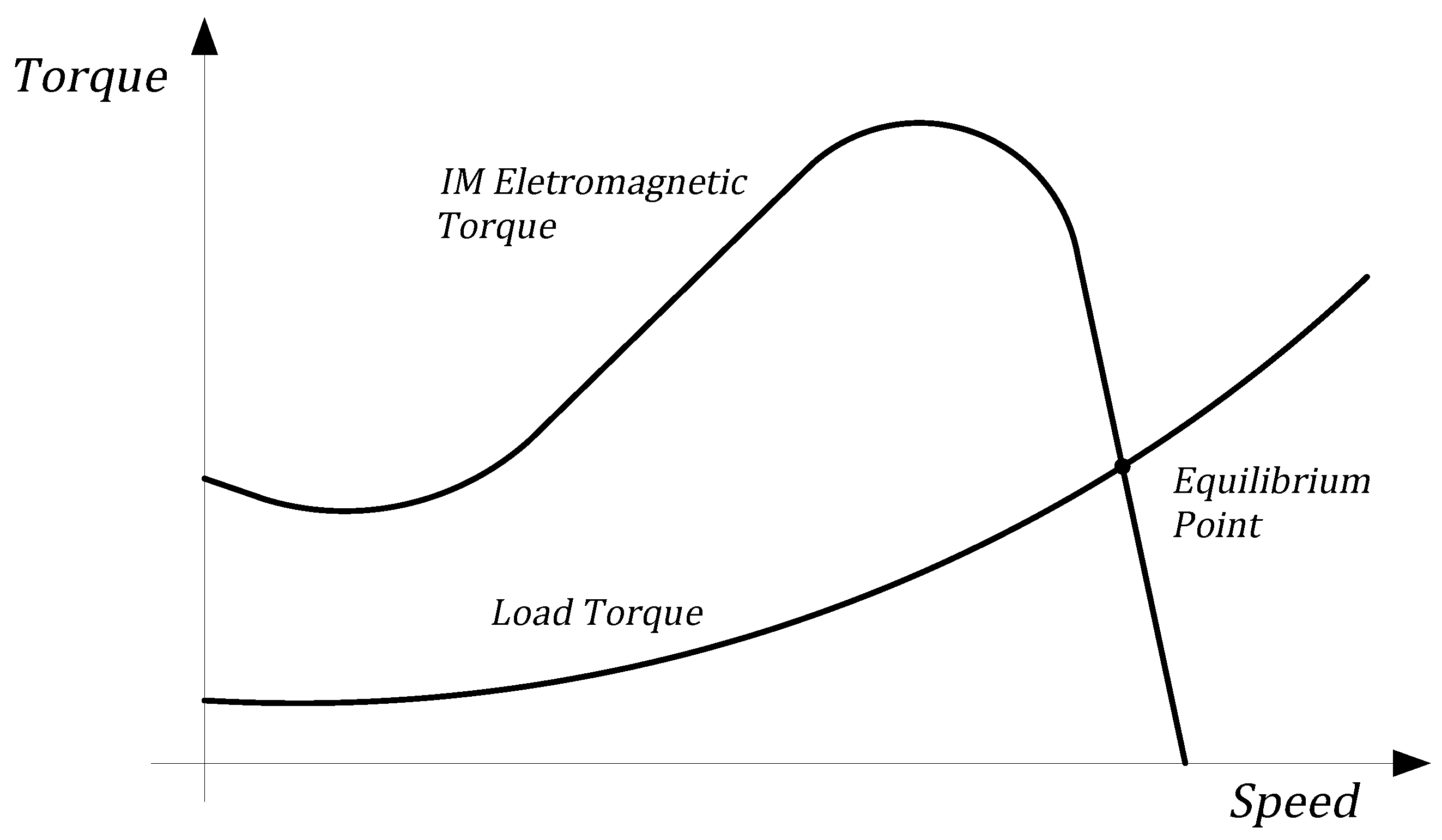
4.4. Steady-State Speed
The steady-state speed of an induction motor is determined by the equilibrium point, where the torque–speed curve of the machine intersects with the load torque curve, indicating a balance between electromagnetic torque, load torque, and friction/windage losses. This equilibrium is illustrated in Figure 4.

Figure 4.
Speed–torque machine curve and a quadratic load torque curve with the operational equilibrium point indicated.
In the dynamic model, steady-state speed is naturally obtained from simulation. When direct-starting a machine with a constant load torque (equal to the nominal motor torque), the motor accelerates until it reaches steady-state speed, where torque equilibrium is achieved.
In the static model, steady-state speed can be determined iteratively by balancing electromagnetic torque with load torque. For a constant load torque, this analysis is straightforward, as the load torque remains constant with speed. By substituting Equation (24) and accounting for friction losses, slip s is given by Equation (33).
For precise slip determination, should include both load torque and windage and frictional torque , as shown in Equation (34).
5. Power Balance in Induction Motors
The induction motor power balance analysis begins with the power conservation rule, as shown in Equation (35). The input power and output power were already defined in Section 4.2 and are not the primary focus of this work.
On the other hand, the power loss term () is often the subject of many papers that aim to understand, classify, and accurately incorporate these losses into induction motor models. In the following subsections, the main motor losses are detailed.
5.1. Stator and Rotor Copper Loss
Stator and rotor copper losses ( and ) result from the Joule effect occurring in the stator and rotor windings, respectively. In both the static and dynamic models, the resistances associated with stator and rotor losses are well defined, making these calculations straightforward in both models. The equations used to determine their values are derived from the classical Joule effect formula, as shown in Equations (36) and (37).
In practical applications, however, the rotor current cannot be directly measured, so its determination relies on the estimator’s accuracy.
5.2. Iron Loss
There is no consensus among researchers on representing iron loss. The primary divergence arises from the fact that this loss varies with both the amplitude and frequency of the supply voltage; thus, a simple resistance with a fixed value may not adequately represent this loss.
However, for this study, we will adopt the typical iron loss resistance representation, as endorsed by the most widely accepted standards: IEEE 112 and IEC 60034-1-2 [1,2]. Referring to the static model equivalent circuit represented in Figure 1, the mathematical equation used to evaluate core loss in both models is shown in Equation (38).
5.3. Stray Load Loss
Stray load loss is the most debated among all loss terms. Even consolidated standards such as IEEE 112 and IEC 60034-1-2 [1,2] differ regarding its definition and calculation methods from a practical perspective.
Its model representation is also controversial, with some authors arguing that it should be positioned in the stator, others in the rotor, and still others debating whether it should be placed in series or parallel with the leakage inductance.
For simplicity and effectiveness, in this work, stray load loss will be represented by a resistance located in the rotor, in series with both the rotor leakage inductance and rotor loss resistance. This approach, aligned with most of the literature, simplifies calculations, as the rotor loss resistance and the stray load loss resistance can be associated or separated as needed for specific applications.
5.4. Windage and Friction Loss
Windage and friction loss represent all the mechanical power that does not contribute to rotor speed. The most significant factors are the viscous friction between the rotor axis and the surrounding air, as well as the power dedicated to ventilating the motor.
In the dynamic model, this loss is explicitly present in the mechanical equation, already described in Equation (14) and repeated here in Equation (39) for convenience.
In the typical static model representation, however, this loss term is accounted for separately. This characteristic makes the static model less suitable for evaluating important motor operational parameters, such as efficiency and mechanical output power. In this work, rotational losses were excluded from the dynamic models to allow a fair comparison between both models.
6. Analysis of a Parameter Set
To implement this analysis, two sets of three-phase induction motor parameters of frequency 60 Hz with four poles with different nominal powers are used to perform the calculations described in Section 4. These sets of parameters are listed in Table 2 and were extracted from [18,19]. Since the referred values were obtained from no-load and rotor-blocked tests, it is known that the rotational losses and core losses are not represented within this set of parameters. The rotational loss is represented by the viscous friction , which is already shown in the motion equation described in Equation (14). The iron loss, on the other hand, is incorporated into the model via the iron loss resistance . This resistance is placed in parallel with the stator inductance and demands almost constant power, as its voltage differs from the supply voltage, also represented in Equation (38) and detailed in Section 5.2.
Table 2.
Three-phase induction motor parameters used in the tests. Both machines are 60 Hz with 4 poles.
It is important to mention that the addition of the parameters and to the model may introduce distortions in the model outputs, resulting in significant differences between the analyzed model and the actual machine that this set of parameters describes. However, in this part of the work, the main objective is to compare two analytical approaches: the dynamic and static models. One of the premises of the analysis is that both models must utilize the same parameter values to highlight the differences between them.
With that said, the determination of the parameter was based on information from [20], which states that core losses represent 20% to 25% of the total losses, and this value increases with nominal power, while the values for parameter were collected from [19], where this information is available for the same set of parameters. Therefore, the value chosen for Motor 1 (3 hp rated power) dissipates approximately 20% of total losses, and for Motor 2 (50 hp rated power), approximately 25% of total losses. The detailed calculations to obtain the resistance are shown in Equations (40)–(42). All variables used are already defined in the previous sections.
Considering a medium value of efficiency around 90%, and the phase voltage as of the rated voltage, the for Motors 1 and 2 is shown in Equations (43).
The procedure for obtaining performance data from the dynamic model involves running the simulation first with the rotor blocked, meaning that the load torque is equal to the torque produced by the machine in every iteration. This step is necessary to collect the starting torque and current without the influence of transient states. This procedure takes exactly 3 s of simulated time for Motor 1 and 4 s for Motor 2, which corresponds to the time required for current stabilization. After this, the machine is released to accelerate until it reaches equilibrium speed, with a load torque equal to its nominal torque. This part of the simulation lasts 2 s, which is sufficient for both motors to accelerate.
In the static model, the procedure is simpler and faster, as it consists of calculating the equivalent circuit impedance to obtain the circuit currents. The steady-state torque, maximum torque, and starting torque are calculated based on the torque equations represented in Equations (24), (25), and (27). A significant detail in the static model calculation is the determination of the steady-state speed, which is not obtained through dynamic equilibrium, as in the dynamic model. Instead, the speed is determined through an iterative calculation using the viscous friction, the load torque, and the torque produced by the motor. However, in this work, the speed obtained from the dynamic simulation is used for the static model, simplifying the procedure and ensuring that both models are evaluated under the same operational conditions.
The main operational parameters, already detailed in Section 4, were collected from the dynamic and static models of the analyzed motors. This information is available in Table 3. The objective is to verify whether the operational data extracted from the models are similar.
Table 3.
Operational parameters collected from dynamic model and static model simulations.
In this table, it can be seen that Motor 1 presents higher variations from the static model to the dynamic model, reaching 9.45% in power factor and 9% in steady-state current. For Motor 2, the same operational parameters exhibit higher variations, but on a smaller scale, reaching 4.36% for power factor and 3.28% for steady-state current.
7. Optimization Algorithm
With the similarities and differences between the dynamic and static models established, an algorithm was developed to determine the induction motor (TIM) parameters based on datasheet information. This algorithm seeks a set of parameters that produces operational data closely resembling those found in the motor datasheet. Given the minimal differences between operational parameters calculated using the static and dynamic models, the static model was selected for its significantly lower computation time.
In this work, the goal was to include as many parameters as possible. Parameters for half-load and three-quarter load were excluded due to the extensive calculations required to determine the machine speed. The remaining datasheet information utilized includes the following:
- Input power;
- Power factor
- Nominal torque
- Starting torque;
- Maximum torque;
- Nominal current;
- Starting current.
The input power is typically not directly available in motor datasheets but can be indirectly calculated from output power and full-load efficiency. This approach is necessary since the efficiency of the machine is not measurable in the static model, as shown in Section 5.
The selected operational parameters were calculated using the equations provided in Section 4. The errors associated with all listed variables were computed using the Equation (44), where denotes the calculated values and denotes the datasheet values.
The total error for optimization or the objective function (OF) was defined as the sum of individual errors , as represented in Equation (45).
where
- N—total number of errors considered;
- i—index for each error to be summed;
- —variable for which the error is being calculated;
- —calculated error of the variable .
7.1. Sine Cosine Algorithm (SCA)
The Sine Cosine Algorithm (SCA) is a population-based metaheuristic optimization method inspired by the mathematical functions of sine and cosine [21]. Introduced by Mirjalili in 2016, it is particularly recognized for effectively balancing exploration and exploitation during the search process [22].
The SCA begins by initializing a population of candidate solutions (agents) randomly within the search space. Each agent iteratively updates its position based on sine and cosine functions, which introduce variability in movement direction and magnitude.
At each iteration, the position of each agent is updated according to its current position and a movement vector influenced by either a sine or cosine function. The general update rule is as follows:
where
- is the position of the i-th agent at iteration k;
- is the position of the best solution (target) at iteration k;
- controls the step size and decreases linearly over iterations to facilitate a transition from exploration to exploitation;
- and are random numbers that modulate the direction and length of the movement, respectively, allowing greater diversity in the search for solutions;
- is a random number that determines whether to use sine or cosine for the update, introducing variations in movement patterns to avoid local minima.
The control parameter is reduced linearly from 2 to 0 over the iterations, promoting a gradual shift from exploration to exploitation. The equation for is given by
where
- k is the current iteration;
- M is the maximum number of iterations.
The SCA explores the search space through wide-ranging sine and cosine oscillations. As the algorithm progresses, the value of decreases, leading to finer, more exploitative searches around the best-known solution. The balance between sine and cosine operations fosters diversity in the search process, allowing the algorithm to explore a broad range of potential solutions initially and converge smoothly toward the optimal solution over time.
7.2. Particle Swarm Optimization (PSO)
Particle Swarm Optimization (PSO) is a population-based optimization technique inspired by the social behavior of birds and fish. Developed by Kennedy and Eberhart in 1995, PSO has become popular for solving various optimization problems due to its simplicity and effectiveness [23].
PSO maintains a swarm of particles, with each particle representing a potential solution to the optimization problem. Each particle moves through the search space based on its own experience and the collective experience of the swarm. The position of each particle is updated iteratively based on two components: its personal best position and the global best position g found by the swarm.
The velocity and position of each particle i at iteration k are updated using the following equations:
where
- is the velocity of particle i at iteration k;
- is the position of particle i at iteration k;
- is the best position found by particle i up to iteration k;
- is the best position found by the swarm up to iteration k;
- W is the inertia weight, controlling the influence of the previous velocity;
- and are acceleration coefficients representing the influence of personal and global best positions;
- and are random numbers uniformly distributed between 0 and 1.
In each iteration, particles are influenced by their previous velocity (exploration) and their attraction to the personal and global best positions (exploitation), ensuring a balance between exploring the search space and exploiting the best-known solutions.
7.3. Comparison of Metaheuristics
The selection of metaheuristics plays a critical role in the optimization algorithm’s performance. This work tests both previously mentioned metaheuristics—the SCA and PSO—operating independently and in a hybrid configuration. The hybrid approach alternates between the two metaheuristics every 50 iterations, leveraging the strengths of both throughout the optimization process.
To compare the effectiveness of these strategies, a straightforward problem was posed to each approach. The operational data presented in Table 3 were input to each metaheuristic five times, aiming to identify the parameter set listed in Table 2. The objective function focused on minimizing the operational data errors described earlier in this section. The results of this comparison are summarized in Table 4.
Table 4.
Comparison between metaheuristics’ performance finding the best set of parameters.
The results demonstrate that the hybrid algorithm is superior to the utilization of the SCA or PSO separately, as it achieved a minimal error of 0.0013, approximately ten times lower than the minimal errors obtained by PSO and seven times lower than the minimal error obtained by the SCA. The average also reflects the hybrid strategy’s superiority, being approximately two times lower than the SCA average and seven times lower than the PSO average.
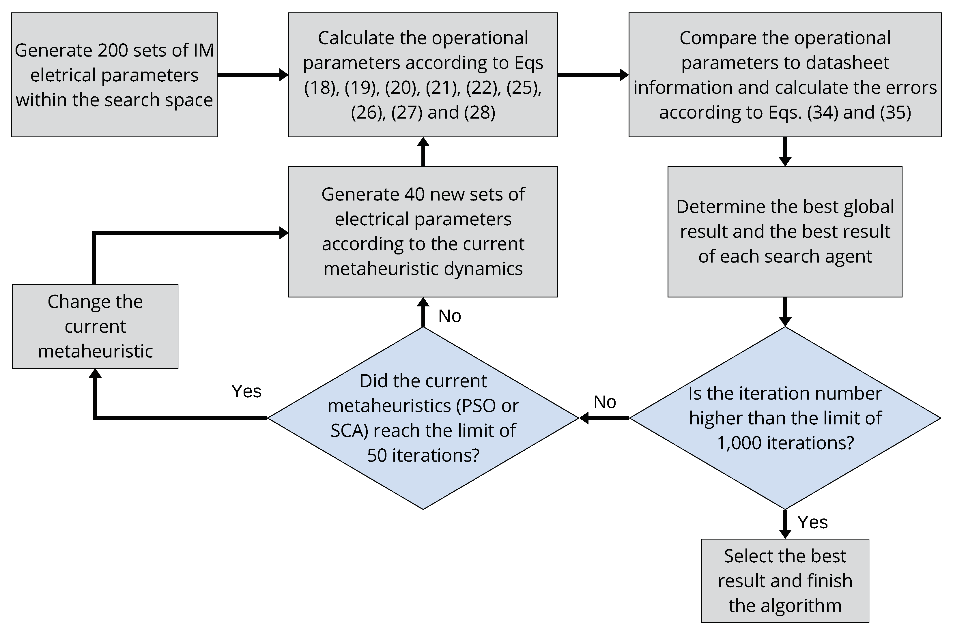
7.4. Proposed Hybrid PSO-SCA Optimization Algorithm (HPSOA)
Building on the previous findings regarding metaheuristic performance, this study introduces the Hybrid PSO-SCA Optimization Algorithm (HPSOA). The algorithm seeks the optimal set of parameters using datasheet information as a reference and alternates between the PSO and SCA metaheuristics. This approach represents an evolution of traditional optimization methods, which typically rely on a single metaheuristic. The core principles of the HPSOA are illustrated in the flowchart in Figure 5.

Figure 5.
Flowchart of the proposed Hybrid PSO-SCA Optimization Algorithm (HPSOA), which alternates the metaheuristic according to the iteration number.
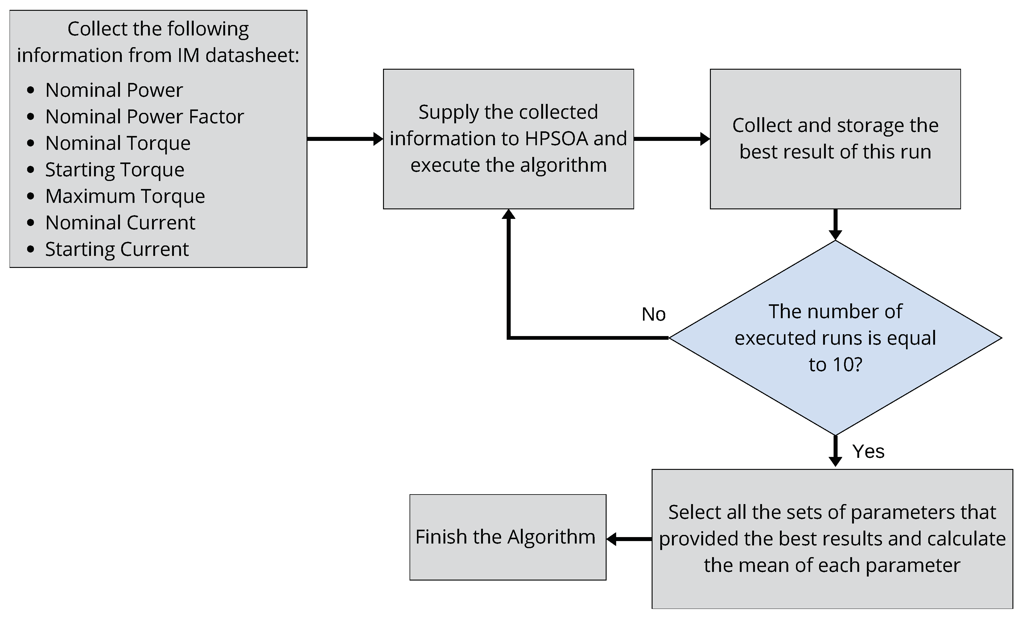
It is important to note that, due to its stochastic nature, the algorithm does not achieve the optimal result in every execution. Consequently, multiple runs are required to ensure the best outcome is obtained. Based on our experiments, 10 executions were sufficient to observe the convergence of the HPSOA and identify the best results. This process is summarized in the workflow depicted in Figure 6, which outlines the steps necessary for users to determine the optimal set of parameters representing the desired induction motor.
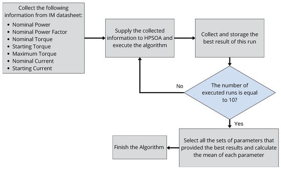
Figure 6.
Flowchart detailing the user workflow to obtain the best set of parameters that represents the studied IM.
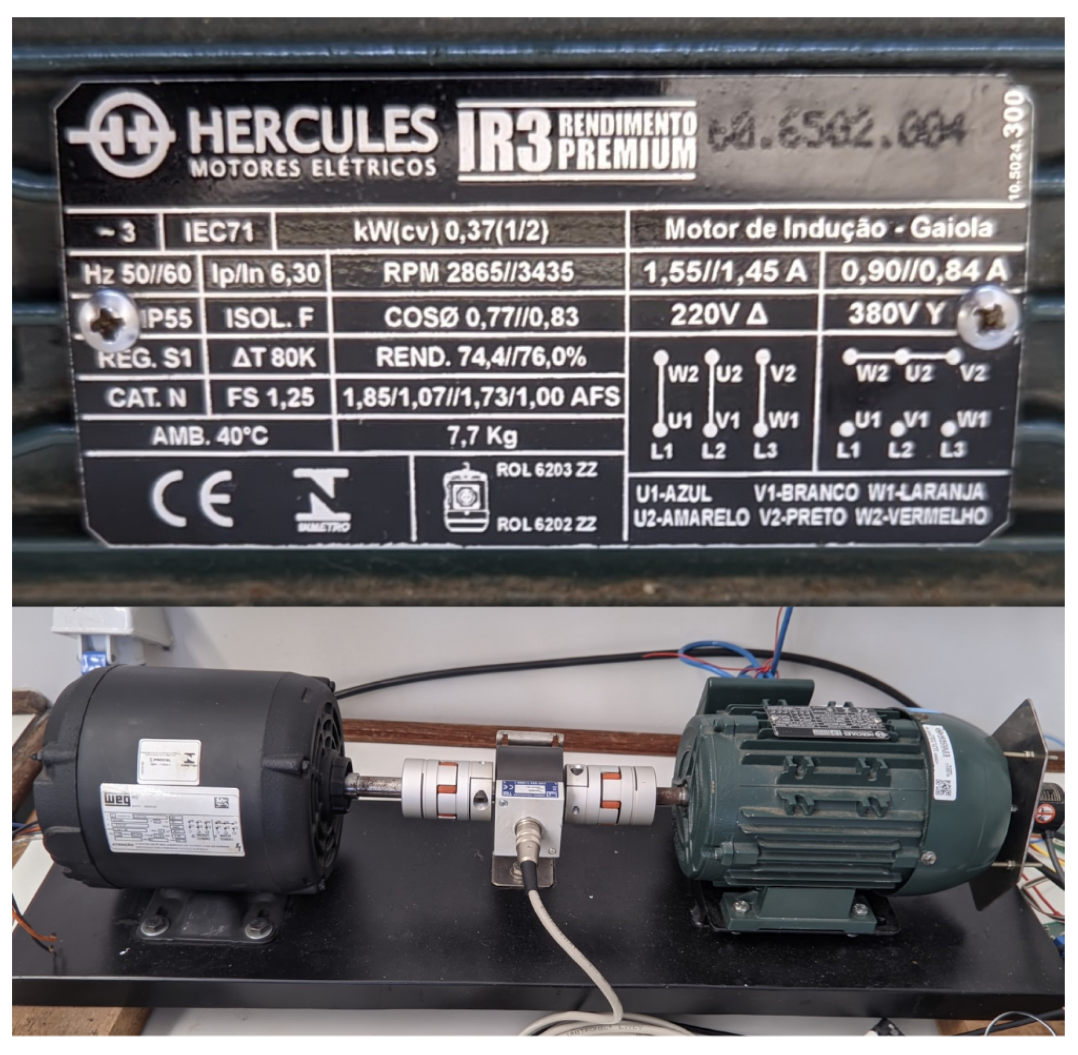
8. Results
The hybrid strategy shown in the previous section was used to estimate the parameters of a real three-phase induction motor based on its operational data available in the manufacturer datasheet. A picture of the used three-phase IM is exhibited in Figure 7, and the datasheet information used to estimate its parameters is listed in Table 5.

Figure 7.
Three-phase induction motor nameplate and the setup used to measure current and speed.
Table 5.
Operational data extracted from manufacturer datasheet of three-phase induction motor used for parameter estimation.
Initially, the model was assumed to have six independent parameters, as suggested in [24] for the “single cage with core loss” model. However, after several executions of the HPSOA algorithm, a significant variation in the stator and rotor leakage inductances ( and ) was observed. To address this issue, the final version of the HPSOA considered a unitary relationship between these inductances, assuming , as usually stated for class A motors.
The optimization algorithm was run ten times to estimate the three-phase IM parameters. The best result obtained in each execution and the parameters obtained in these executions are listed in Table 6. As one can see, all runs presented a very good convergence, with very low variations. Once the error value obtained in all 10 runs is the same, all executions are considered and the final result is calculated as the average of the obtained parameters, shown in Table 7.
Table 6.
Optimization results of ten executions of the hybrid optimization algorithm.
Table 7.
Average of the parameters obtained only from the executions that reached the best result.
In Table 8, the operational data obtained from the mentioned parameters and the expected data, extracted from the datasheet, are listed.
Table 8.
Operational data obtained from manufacturer datasheet and from static model simulated with estimated parameters.
The results shown in Table 6 demonstrate that even when comparing the results using a static model, the operational parameters suffer some variations, indicating the model’s inability to fit all operational data simultaneously.
Validation with Real Motor
The presented results show that the optimization algorithm converged to a set of parameters whose operational data calculated from the static model coincide with operational data collected from the datasheet. However, verification with a real motor must be carried out to validate the procedure.
To make this comparison, a free acceleration test was performed with the real motor, and the obtained parameters were used to simulate the same free acceleration test. The collected parameters from this test were starting current and current and speed with no load.
The first challenge to implement a free acceleration test with the parameters obtained is to determine the mechanical parameters that are not covered by the static model. The strategy was to simulate with typical values of momentum of inertia (J) and viscous friction and analyze the equilibrium speed. After some tests, the best value was and . Using lower values than these, the steady-state behavior was unstable, and for higher values, the no-load speed was lower than that observed in the real motor.
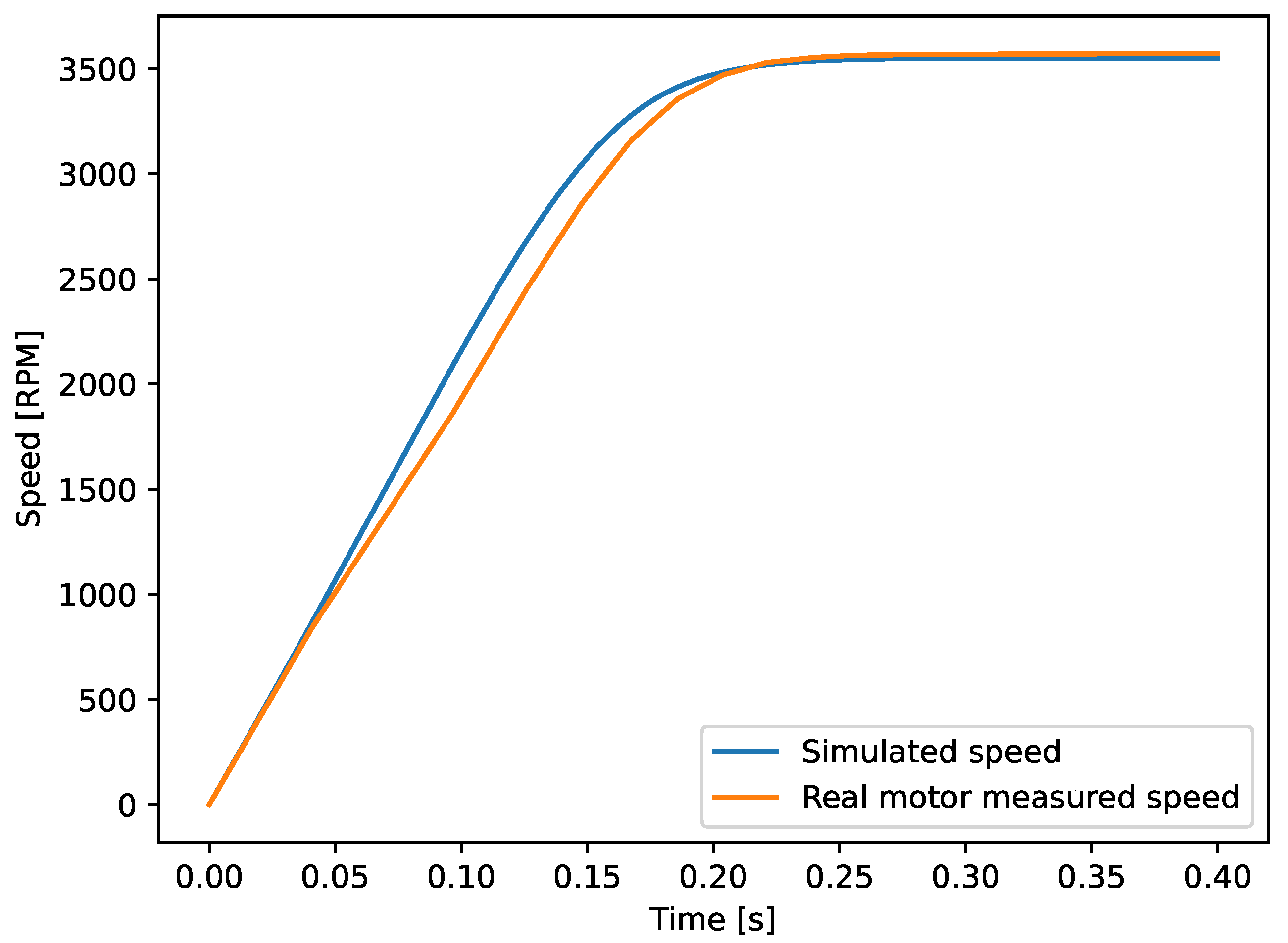
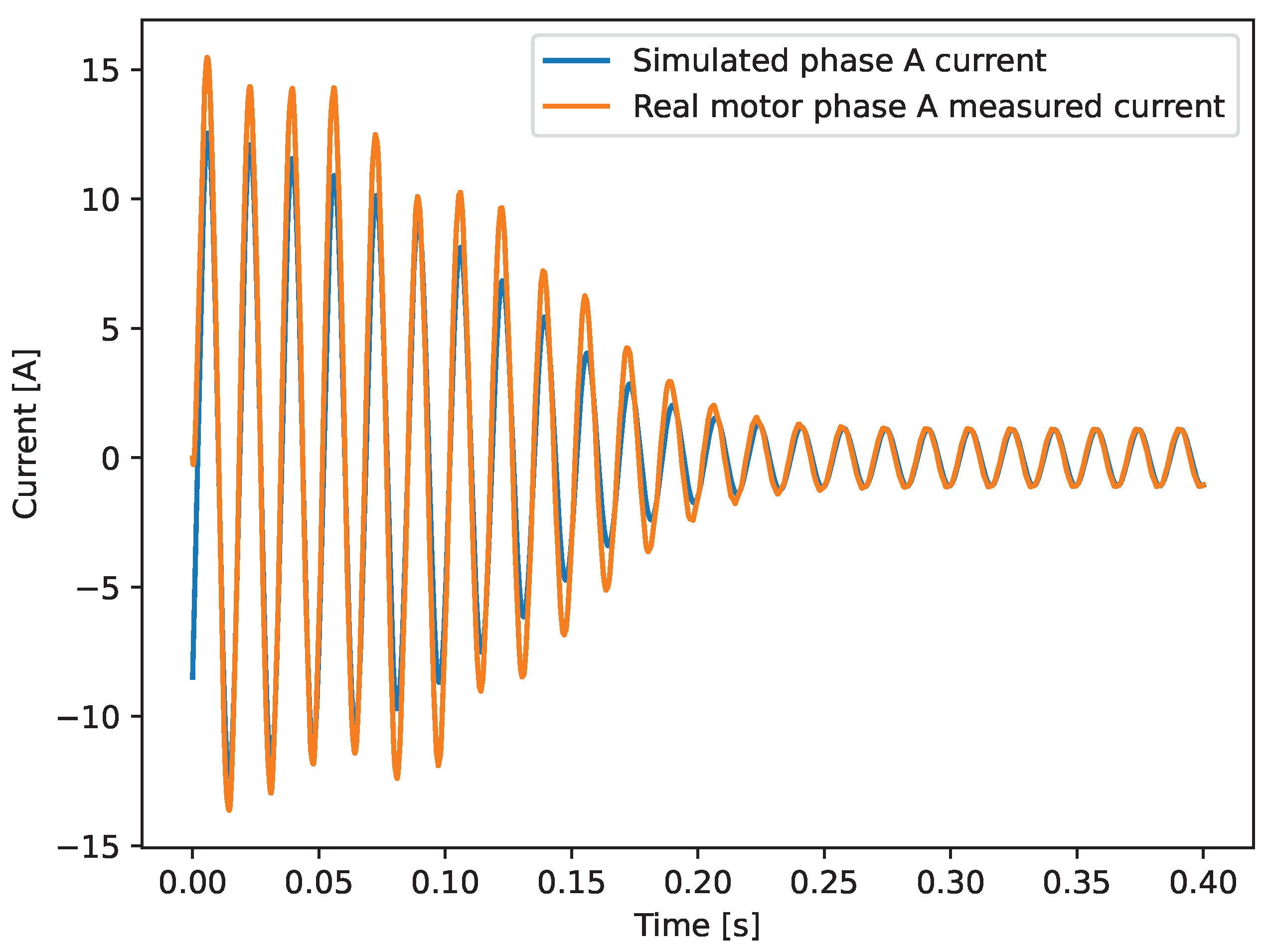
After this first adjustment, a simulation with the optimal parameters was run, and a no-load test with the real motor was made. The collected speed and phase A current signals for the real motor and the simulation are shown in Figure 8 and Figure 9. To quantify the errors observed in these graphs, it is essential to assess how well the simulated signal aligns with the measured one. For the speed signal, which is always positive and converges to a steady-state value after a certain simulation time, the error is calculated according to Equation (51).
where
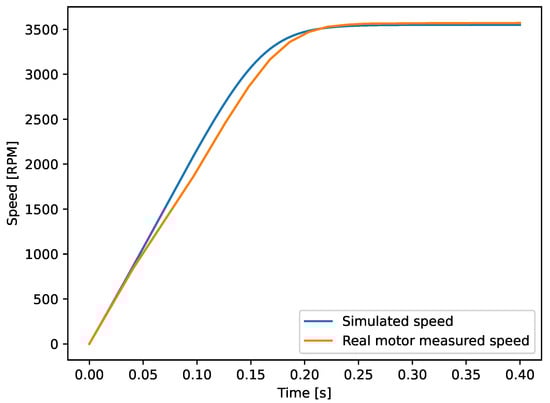
Figure 8.
Measured speed and simulated speed with estimated parameters.
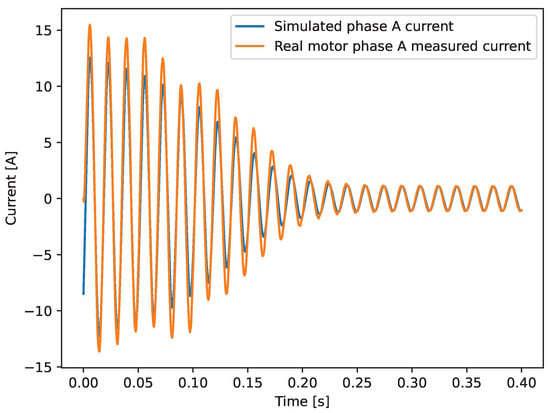
Figure 9.
Measured current and simulated current with estimated parameters.
- —speed error;
- —j-th sample of simulated speed signal;
- —j-th sample of measured speed signal.
For the current signals, however, the oscillatory nature of the waveform distorts the error calculation according to Equation (51). Thus, the most effective error calculation strategy identified by the authors is a direct comparison of the traditional root mean square (RMS) values. The performed RMS calculation is described here in Equation (52) for a generic variable X, while the current error that relies on the RMS values of current is shown in Equation (53).
where
- —current error;
- —RMS value of simulated current signal;
- —RMS value of measured current signal.
As illustrated in Figure 9, the error is notably higher during the starting interval compared to the steady-state region. This variation makes a single error measurement for the entire signal unsuitable for in-depth analysis. To address this limitation, the RMS values for the current are calculated separately for the starting and steady-state regions. The starting region is defined as the time interval from the beginning of the simulation (t = 0 s) until t = 0.25 s (corresponding to 15 wavecycles for a 60 Hz system), while the steady-state region is defined as the time between t = 0.25 s and t = 0.4 s. The error of speed signal and of current signals is summarized in Table 9.
Table 9.
Speed error and current error for starting current (from t = 0 s to t = 0.25 s) and steady-state current (from t = 0.25 s to t = 0.4 s).
Other important measurements of error are the steady-state speed, steady-state RMS current, and starting RMS current. These parameters do not evaluate the fitting of the curves, but help to understand the similarity of both systems. These data are presented in Table 10.
Table 10.
Comparison of measurements made in real motor with results obtained from simulation using the estimated parameters.
9. Discussion
The comparison between the static and dynamic models developed in this study revealed that both approaches provide comparable information for most of the operational parameters analyzed, excepting the steady-state current and power factor, which presented higher level of errors when compared to the others. Once the parameters used in both models are the same and the speed is also the same, this difference should be addressed in future works, to make a deeper investigation concerning this deviation.
However, considering that most of the operational parameters presented high coherence in both models, the static model was chosen to perform the simulations. This option provides faster computations, allowing a higher number of simulations with the same computational power.
Additionally, the performance of two metaheuristics, PSO and the SCA, was evaluated and compared with the proposed Hybrid PSO-SCA Optimization Algorithm (HPSOA). The results demonstrated that the HPSOA significantly outperformed the other algorithms in terms of optimization efficiency and accuracy.
Using these insights, the HPSOA was applied to estimate the electrical parameters of a 0.5 hp three-phase induction motor. After 10 executions, the algorithm consistently converged to optimal solutions.
The parameters obtained through the HPSOA were validated against the motor corresponding to the datasheet used in the optimization process. Validation results confirmed the accuracy of the HPSOA, with errors of approximately 0.58% for steady-state simulated speed and about 3.5% for phase A steady-state current. The higher error observed in the starting current is attributed to limitations inherent in the single-cage IM model, a phenomenon well documented in the literature [25,26].
10. Conclusions and Future Works
This study has provided valuable insights into the dynamic and static models of three-phase induction motors. While the evaluated operational parameters showed general consistency, some differences were observed, underscoring the need for further investigation. Specifically, the use of a static model to infer conclusions about observers based on state-space models may introduce deviations, necessitating careful consideration and planning.
The proposed HPSOA was employed to estimate the parameters of a 0.5 hp three-phase induction motor using datasheet information. The results demonstrated good alignment with the real motor dynamics during a free acceleration test, achieving an error of 0.58% in speed and 3.75% in steady-state phase currents. The higher error observed in the starting current is attributed to the limitations of the single-cage model.
For future research, the authors recommend a more comprehensive analysis of dynamic and static models by expanding the range of motors evaluated in terms of type and power. Additionally, comparing the performance of different models, such as the double-cage model with core losses, could help further reduce discrepancies between static and dynamic models, particularly with respect to the induction motor’s starting current. Investigating the linear dependency of the “single cage model with core loss” model parameters used in this work also represents a promising research direction. Furthermore, this study has demonstrated that the proposed HPSOA offers robust convergence and highly accurate results, making it a promising tool for future investigations.
Author Contributions
Conceptualization, N.H.B.S., I.Y., F.D.C.O., D.S.L.S. and H.R.O.R.; methodology, N.H.B.S., I.Y., F.D.C.O., D.S.L.S. and H.R.O.R.; software, N.H.B.S. and H.R.O.R.; validation, F.D.C.O., A.E.A.A. and H.R.O.R.; formal analysis, N.H.B.S., F.D.C.O. and H.R.O.R.; investigation, N.H.B.S.; resources, F.D.C.O. and D.S.L.S.; data curation, N.H.B.S., F.D.C.O. and A.E.A.A.; writing—original draft preparation, N.H.B.S.; supervision, N.H.B.S. and F.D.C.O.; project administration, N.H.B.S., F.D.C.O., D.S.L.S. and H.R.O.R.; funding acquisition, N.H.B.S. and H.R.O.R. All authors have read and agreed to the published version of the manuscript.
Funding
This research was funded by the Fundação de Amparo à Pesquisa e Inovação do Espírito Santo, grant numbers FAPES-2022-BWBR2 and FAPES-2021-B6WSC, and the Conselho Nacional de Desenvolvimento Científico e Tecnológico, grant number CNPq-309737/2021-4, CNPq-309823/2018-8, NiDA, PREDFLEX-CM project (TEC-2024/ECO-287), through the R&D activities programme “Tecnologías 2024” funded by Madrid state, and the project PVCAD funded by the Spanish ministry of sciences, innovation and universities (PID2023-151697OA-100).
Data Availability Statement
Dataset available on request from the authors.
Conflicts of Interest
The authors declare no conflicts of interest.
References
- IEEE 112:2017; IEEE Standard Procedure for Polyphase Induction Motors and Generators. Standard, Institute of Electrical and Electronics Engineers: New York, NY, USA, 2017.
- IEC 60034-2-1; Rotating Electrical Machines-Part 2-1: Standard Methods for Determining Losses and Efficiency from Tests (Excluding Machines for Traction Vehicles). Standard, International Electrotechnical Commission: Geneva, Switzerland, 2020.
- Pedra, J.; Corcoles, F. Estimation of induction motor double-cage model parameters from manufacturer data. IEEE Trans. Energy Convers. 2004, 19, 310–317. [Google Scholar] [CrossRef]
- Lindenmeyer, D.; Dommel, H.; Moshref, A.; Kundur, P. An induction motor parameter estimation method. Int. J. Electr. Power Energy Syst. 2001, 23, 251–262. [Google Scholar] [CrossRef]
- Torrent, M. Estimation of equivalent circuits for induction motors in steady state including mechanical and stray load losses. Eur. Trans. Electr. Power 2012, 22, 989–1015. [Google Scholar] [CrossRef]
- Barut, M.; Bogosyan, S.; Gokasan, M. Speed-sensorless estimation for induction motors sing extended Kalman filters. IEEE Trans. Ind. Electron. 2007, 54, 272–280. [Google Scholar] [CrossRef]
- Yildiz, R.; Barut, M.; Zerdali, E. A Comprehensive Comparison of Extended and Unscented Kalman Filters for Speed-Sensorless Control Applications of Induction Motors. IEEE Trans. Ind. Inform. 2020, 16, 6423–6432. [Google Scholar] [CrossRef]
- Rodriguez, J.; Cortes, P. Predictive Control of Power Converters and Electrical Drives, 1st ed.; John Wiley & Sons, Inc.: Hoboken, NJ, USA, 2012; p. 230. [Google Scholar]
- Fitzgerald, A.E. Electric Machinery, 6th ed.; McGraw-Hill: New York, NY, USA, 2003; p. 688. [Google Scholar]
- Amaral, G.F.V.; Baccarini, J.M.R.; Coelho, F.C.R.; Rabelo, L.M. A High Precision Method for Induction Machine Parameters Estimation From Manufacturer Data. IEEE Trans. Energy Convers. 2021, 36, 1226–1233. [Google Scholar] [CrossRef]
- Lima, S.C.; Wengerkievicz, C.A.C.; Batistela, N.J.; Sadowski, N.; da Silva, P.A.; Beltrame, A.Y. Induction motor parameter estimation from manufacturer data using genetic algorithms and heuristic relationships. In Proceedings of the 2017 Brazilian Power Electronics Conference (COBEP), Juiz de Fora, Brazil, 19–22 November 2017; pp. 1–6. [Google Scholar] [CrossRef]
- Accetta, A.; Alonge, F.; Cirrincione, M.; D’Ippolito, F.; Pucci, M.; Sferlazza, A. GA-Based Off-Line Parameter Estimation of the Induction Motor Model Including Magnetic Saturation and Iron Losses. IEEE Open J. Ind. Appl. 2020, 1, 135–147. [Google Scholar] [CrossRef]
- Vukašinović, J.; Štatkić, S.; Milovanović, M.; Arsić, N.; Perović, B. Combined method for the cage induction motor parameters estimation using two-stage PSO algorithm. Electr. Eng. 2023, 105, 2703–2714. [Google Scholar] [CrossRef]
- Ipek, S.N.; Taskiran, M.; Bekiroglu, N.; Aycicek, E. Optimal induction machine parameter estimation method with artificial neural networks. Electr. Eng. 2024, 106, 1959–1975. [Google Scholar] [CrossRef]
- Khoury, G.; Ghosn, R.; Khatounian, F.; Fadel, M.; Tientcheu, M. An improved dynamic model for induction motors including core losses. In Proceedings of the 2016 IEEE International Power Electronics and Motion Control Conference (PEMC), Varna, Bulgaria, 25–28 September 2016; pp. 526–531. [Google Scholar] [CrossRef]
- Khoury, G.; Ghosn, R.; Khatounian, F.; Fadel, M.; Tientcheu, M. Energy-efficient field-oriented control for induction motors taking core losses into account. Electr. Eng. 2021, 104, 529–538. [Google Scholar] [CrossRef]
- Sen, P.C. Principles of Electric Machines and Power Electronics, 3rd ed.; Wiley: Hoboken, NJ, USA, 2014; p. 618. [Google Scholar]
- Krause, P.; Wasynczuk, O.; Sudhoff, S. Analysis of Electric Machinery and Drive Systems, 2nd ed.; John Wiley & Sons, Inc.: Hoboken, NJ, USA, 2002. [Google Scholar]
- Cathey, J.J.; Cavin, R.K.; Ayoub, A.K. Transient Load Model of an Induction Motor. IEEE Trans. Power Appar. Syst. 1973, PAS-92, 1399–1406. [Google Scholar] [CrossRef]
- de Almeida, A.T.; Ferreira, F.J.T.E.; Baoming, G. Beyond Induction Motors—Technology Trends to Move Up Efficiency. IEEE Trans. Ind. Appl. 2014, 50, 2103–2114. [Google Scholar] [CrossRef]
- Mirjalili, S. SCA: A Sine Cosine Algorithm for solving optimization problems. Knowl.-Based Syst. 2016, 96, 120–133. [Google Scholar] [CrossRef]
- Houssein, E.H.; Saeed, M.K.; Hu, G.; Al-Sayed, M.M. Metaheuristics for Solving Global and Engineering Optimization Problems: Review, Applications, Open Issues and Challenges. Arch. Comput. Methods Eng. 2024, 96. [Google Scholar] [CrossRef]
- Kennedy, J.; Eberhart, R. Particle swarm optimization. In Proceedings of the ICNN’95-International Conference on Neural Networks, Perth, WA, Australia, 27 November–1 December 1995; Volume 4, pp. 1942–1948. [Google Scholar] [CrossRef]
- Corcoles, F.; Pedra, J.; Salichs, M.; Sainz, L. Analysis of the induction machine parameter identification. IEEE Trans. Energy Convers. 2002, 17, 183–190. [Google Scholar] [CrossRef]
- Pedra, J.; Candela, I.; Sainz, L. Modelling of squirrel-cage induction motors for electromagnetic transient programs. IET Electr. Power Appl. 2009, 3, 111–122. [Google Scholar] [CrossRef]
- Ćalasan, M.; Micev, M.; Ali, Z.M.; Zobaa, A.F.; Abdel Aleem, S.H.E. Parameter Estimation of Induction Machine Single-Cage and Double-Cage Models Using a Hybrid Simulated Annealing–Evaporation Rate Water Cycle Algorithm. Mathematics 2020, 8, 1024. [Google Scholar] [CrossRef]

Disclaimer/Publisher’s Note: The statements, opinions and data contained in all publications are solely those of the individual author(s) and contributor(s) and not of MDPI and/or the editor(s). MDPI and/or the editor(s) disclaim responsibility for any injury to people or property resulting from any ideas, methods, instructions or products referred to in the content. |
© 2025 by the authors. Licensee MDPI, Basel, Switzerland. This article is an open access article distributed under the terms and conditions of the Creative Commons Attribution (CC BY) license (https://creativecommons.org/licenses/by/4.0/).