Optimization Model-Based Robust Method and Performance Evaluation of GNSS/INS Integrated Navigation for Urban Scenes

Abstract

The robust and high-precision estimation of position and attitude information using a combined global navigation satellite system/inertial navigation system (GNSS/INS) model is essential to a wide range of applications in intelligent driving and smart transportation. GNSS systems are susceptible to inaccuracies and signal interruptions in occluded environments, which lead to unreliable parameter estimations in GNSS/INS based on filter models. To address this issue, in this paper, a GNSS/INS combination model based on factor graph optimization (FGO) is investigated and the robustness of this optimization model is evaluated in comparison to the traditional extended Kalman filter (EKF) model and robust Kalman filter (RKF) model. In this paper, both high- and low-accuracy GNSS/INS combination data are used and the two sets of urban scene data are collected using high- and low-precision consumer-grade inertial guidance systems and an in-vehicle setup. The experimental results demonstrate that the position, velocity, and attitude estimates obtained using the GNSS/INS and the FGO model are superior to those obtained using the traditional EKF and robust EKF methods. In the simulated scenarios involving gross interference and GNSS signal loss, the FGO model achieves optimal results. The maximum improvement rates of the position, velocity, and attitude estimates are 81.1%, 73.8%, and 75.1% compared to the EKF method and 79.8%, 72.1%, and 57.1% compared to the RKF method, respectively.

1. Introduction

Global navigation satellite systems (GNSS), which are capable of providing continuously available high-precision positioning information on the global scale [1], have been widely used to determine spatial and temporal information about various carriers such as land, sea, and air [2]. High-precision and reliable positioning in urban environments is crucial to applications such as intelligent driving and smart transportation, and GNSS technology has become a prevalent choice for high-precision urban positioning due to its ability to rapidly deliver absolute position information. However, in urban environments containing numerous high-rise buildings, tunnels, viaducts, and trees, GNSS signals are often obstructed or reflected. This leads to significant multipath and non-line-of-sight issues, as well as frequent gross errors and cycle slips, which compromise the accuracy and reliability of GNSS positioning [3]. Inertial navigation systems (INS) can provide high-precision position information over short periods of time as they are not affected by external environmental factors. Combining GNSS with INS can address the limitations of each of these systems. Consequently, many researchers have explored the use of GNSS/INS integration algorithms to enhance positioning accuracy and reliability in complex urban settings [4,5].

The extended Kalman filter (EKF) is a common parameter estimation method for GNSS/INS combinations [6]. Inaccurate a priori stochastic and observational models can affect the accuracy of the parameter estimation of the EKF method [7]. In urban scenarios, phenomena such as multipath effects and non-line-of-sight signals can interfere with GNSS signals, leading to bias in the combined GNSS/INS navigation parameters based on the EKF model. To improve the parameter estimation accuracy of the combined system in GNSS signal fading scenarios, many scholars have investigated the use of a combination of the GNSS/INS model, the adaptive Kalman filter (AKF), and the robust Kalman filter [8,9]. The AKF can be implemented using different methods, such as the Bayesian, maximum likelihood, correlation, and covariance matching methods. Sage and Husa proposed the well-known Sage–Husa adaptive filter algorithm to solve the problem of unknown a priori statistical information of system noise [10], and it has since become a widely used adaptive filter algorithm [11,12]. Based on the theory of robust estimation, scholars have proposed many classical biased functions, such as the Hampel function, the Tukey function, the Huber function [13], and the IGGIII function [14]. To overcome the limitation of inaccurate statistical characteristics of navigation system noise, Gao et al. developed a robust adaptive filter algorithm that adaptively adjusts the covariance matrix of the system state noise based on an adaptive factor constructed from predicted residuals [15]. Guo et al. improved an adaptive robust Kalman filter based on the theory of travel hypothesis testing that can effectively improve the positioning performance of the combined GNSS/INS system [16]. Yin proposed an adaptive robust Kalman filter algorithm based on PDOP values that is robust in complex urban scenarios [17]. Nevertheless, combined GNSS/INS navigation based on the AKF and RKF only uses observation and prediction information at the current moment for coarse detection and processing and does not fully utilize historical observation information.

In contrast, the factor graph optimization (FGO) method makes full use of historical observations and suppresses the effects of coarseness by updating the linearization points through repeated iterations [18]. Kschischang et al. introduced the concept of factor graphs, providing a theoretical basis for subsequent studies [19]. Dellaert et al. introduced the FGO method as an optimization method for navigation problems [20], and graph optimization is now a commonly used estimator for back-end optimization [21]. They won first place in Google’s smartphone decimeter positioning competition for the second consecutive year using a factor graph optimization model [22,23], which demonstrates the feasibility of using graph optimization for GNSS positioning. Xin et al. constructed a combined precise point positioning-B2b-INS (PPP-B2b/INS) to loosely model the EKF and FGO algorithms, and they investigated the positioning performance of the two parameter estimation models in occluded scenarios such as urban roads and overpass scenes. Their results demonstrate that the FGO algorithm outperforms the EKF algorithm in terms of positioning [24]. Zhang et al. constructed a single-difference GNSS model based on the FGO model and they used outlier detection and the partial fuzziness resolution to ensure the urban positioning performance. Their results proved that, compared to the EKF, the FGO improves positioning accuracy and reliability [25]. Wen et al. showed that the positioning performances of GNSS/INS which loosely and tightly combined models based on the FGO algorithm are better than that of the traditional EKF algorithm, and they explored the effect of the window size on the performance of the FGO. Their results demonstrate that the appropriate window size is highly correlated with the environmental conditions [26]. GNSS observations in urban occlusion scenarios are susceptible to contamination, which in turn affects the performance of the combined GNSS/INS system. To improve the parameter estimation performance of the loose GNSS/INS combination model in urban occlusion environments, Li et al. constructed an adaptive FGO combination model supported by a convolutional neural network and verified that the modified algorithm’s positioning performance is better than those of the EKF and AKF models in urban occlusion scenarios [27]. Hu et al. implemented a robust graph optimization method for shipboard GNSS/INS combination by constructing an anti-differential GNSS factor based on pseudorange observations and an inertial measurement unit (IMU) factor. Their results demonstrate that the positioning accuracy of this anti-differential optimization method is better than those of the FGO and EFK models in occluded scenarios [28]. Zhang et al. studied the performance of INS assisted positioning in GNSS denial environments, effectively providing guidance for GNSS/INS in GNSS denial environments [29].

Currently, most researchers have examined the robust performance of GNSS/INS combined navigation parameter estimation using the FGO method in urban scenarios. These studies primarily compared the FGO method with traditional combined navigation results based on the EKF method, and they often did not evaluate the anti-discrepancy performances of both high- and low-cost navigation equipment when using the EKF, RKF, and FGO algorithms under complex conditions. It is necessary to conduct GNSS/INS experimental analysis through high- and low-precision inertial navigation to compare the positioning performance of KF and FGO algorithms in conventional environments, gross error environments, and GNSS denial environments. Therefore, in this study, we investigated the loosely coupled GNSS PPP and INS combination models based on the EKF, RKF, and FGO algorithms for in-vehicle systems in urban environments utilizing both high- and low-cost devices. We analyzed the parameter estimation performances of the loosely coupled GNSS PPP/INS combination models under occluded environments using the EKF, RKF, and FGO methods. The remainder of this paper is organized as follows: Section 1 describes the loosely coupled GNSS PPP/INS combination models based on the EKF, RKF, and FGO algorithms. Section 2 presents the data collected from a vehicle-mounted GNSS/INS combination system using both high- and low-precision equipment and experimentally analyzes the algorithms. Section 3 presents the experimental conclusions.

2. Models and Methods

In this paper, we investigate three GNSS PPP/INS integration navigation models based on the GNSS PPP ionosphere-free model. The three models include the loosely coupled GNSS PPP/INS model based on the EKF model, the loosely coupled GNSS PPP/INS model based on RKF model, and the loosely coupled GNSS PPP/INS model based on factor graphs [30]. These three algorithms are described in this section.

2.1. Robust Extended Kalman Filter Loosely Coupled GNSS PPP/INS Models

2.1.1. State Model

The loosely combined PPP/INS error model is derived from the INS error model, and the Phi angle model error can be expressed as follows [31]:

$$\left\{\begin{array}{c}{\dot{\mathit{\phi }}}^n=-{\mathit{\omega }}_{in}^n\times {\mathit{\phi }}^n+\Delta {\mathit{\omega }}_{in}^n-C_b^n\Delta {\mathit{\omega }}_{ib}^b\\ \Delta {\dot{v}}^n=f^n\times {\mathit{\phi }}^n-(2{\mathit{\omega }}_{ie}^n+{\mathit{\omega }}_{en}^n)\times \Delta v^n-(2\Delta {\mathit{\omega }}_{ie}^n+\Delta {\mathit{\omega }}_{en}^n)\times v^n+C_b^n\Delta f^b+\Delta g^n\\ \Delta {\dot{r}}^n=F_{rr}\Delta r^n+F_{rv}\Delta v^n\end{array}\right.i$$

(1)

where n is the navigation coordinate system, $i$ is the inertial coordinate system, b is the body coordinate system, e is the Earth-centered Earth-fixed (ECEF) coordinate system, ${\mathit{\phi }}^{\mathrm{n}}$, $\Delta v^n$, and $\Delta r^n$ are the attitude, velocity, and position errors, ${\mathit{\omega }}_{\mathit{i}\mathit{n}}^{\mathit{n}}$ = ${\mathit{\omega }}_{\mathit{i}\mathit{e}}^{\mathit{n}}$ + ${\mathit{\omega }}_{\mathit{e}\mathit{n}}^{\mathit{n}}$, ${\mathit{\omega }}_{\mathit{i}\mathit{e}}^{\mathit{n}}$ is the angular velocity of the e-frame relative to the i-frame, ${\mathit{\omega }}_{\mathit{e}\mathit{n}}^{\mathit{n}}$ is the angular velocity of the e-frame relative to the n-frame, ${\mathit{\omega }}_{\mathit{i}\mathit{b}}^{\mathit{b}}$ is the angular velocity output of the gyroscope in the b-frame, ${\mathit{C}}_{\mathit{b}}^{\mathit{n}}$ is the direction cosine matrix from the b-frame to the n-frame, ${\mathit{f}}^{\mathit{b}}$ is the specific force, $\Delta {\mathit{g}}^{\mathit{n}}$ is the gravity error, and ${\mathit{F}}_{\mathit{r}\mathit{r}}$ and ${\mathit{F}}_{\mathit{r}\mathit{v}}$ are the corresponding coefficient matrixes.

In this paper, we establish a 15-dimension state equation using the attitude angles, velocity, position, gyroscope bias, accelerometer bias, and scale factor errors as state variables. The equation is as follows:

$$\dot{x}(t)=F\left(t\right)x\left(t\right)+G\left(t\right)w\left(t\right)$$

(2)

where $\mathit{x}\left(\mathit{t}\right)={\left[{\left(\Delta {\mathit{r}}_{\mathit{I}\mathit{N}\mathit{S}}^{\mathit{n}}\right)}^{\mathit{T}}\hspace{1em}{\left(\Delta {\mathit{v}}_{\mathit{I}\mathit{N}\mathit{S}}^{\mathit{n}}\right)}^{\mathit{T}}\hspace{1em}{\mathit{\varphi }}^{\mathit{T}}\hspace{1em}{\mathit{b}}_{\mathit{g}}^{\mathit{T}}\hspace{1em}{\mathit{b}}_{\mathit{a}}^{\mathit{T}}\right]}^{\mathit{T}}$, $F\left(t\right)$ is the coefficient matrix of the system state variables, $G\left(t\right)$ is the noise driving matrix, and $\mathit{w}\left(\mathit{t}\right)$ is the system noise.

2.1.2. Observation Model

In this paper, we investigate the GNSS PPP/INS loosely integrated model, in which the position information obtained from the GNSS PPP calculations and the position information predicted by the INS are used to construct the observation model. Typically, the center of the GNSS antenna does not align with the center of the IMU, which results in a lever arm effect. The measurement equation for the PPP/INS loosely integrated model, which accounts for the lever arm effect, is as follows:

$$Z_k=\left[r_{PPP}^n-\left(r_{INS}^n-D{C}_b^n{l}^b\right)\right]=H_k{X}_k+{\mathit{\eta }}_k$$

(3)

where ${\mathit{Z}}_{\mathit{k}}$ is the observation vector, ${\mathit{r}}_{\mathit{P}\mathit{P}\mathit{P}}$ is the position information computed using the GNSS PPP, and ${\mathit{r}}_{\mathit{I}\mathit{N}\mathit{S}}$ is the position information predicted by the INS. $\mathit{D}$ is the rotation matrix that transforms the lever arm ${\mathit{l}}^{\mathit{b}}$ from the n-frame to the geographic coordinate system, and ${\mathit{\eta }}_{\mathit{k}}$ is the observation noise. ${\mathit{H}}_{\mathit{k}}$ is the coefficient matrix of the observation equation, which considers the lever arm effect. The coefficient matrix of the observation equation can be expressed as follows:

$$H_k=\left[I_{\mathbf{3}}\hspace{1em}{\mathbf{0}}_{\mathbf{3}}\hspace{1em}\left(C_b^n{l}^b\times \right)\hspace{1em}{\mathbf{0}}_{\mathbf{3}}\hspace{1em}{\mathbf{0}}_{\mathbf{3}}\hspace{1em}{\mathbf{0}}_{\mathbf{3}}\hspace{1em}{\mathbf{0}}_{\mathbf{3}}\right]$$

(4)

where $\mathit{I}$ is the identity matrix.

2.1.3. Robust EKF Based on the Observation Residuals

Considering the nonlinearity of GNSS PPP/INS integrated navigation, the EKF model is employed to solve Equations (2) and (3). In urban environments, GNSS observations are often contaminated, which leads to deviations in the positioning results. To mitigate the impact of low-quality observations on GNSS PPP/INS integrated navigation, the robust EKF is commonly used [14,17]. The robust EKF method detects low-quality observations through residuals and adjusts their variance using robust factors, which reduces their influence on the integrated navigation solution.

The EKF algorithm is a recursive process comprising initialization, state prediction, and measurement update processes. During initialization, the state vector $\mathit{x}$, its covariance matrix $\mathit{P}$, the process noise matrix $\mathit{Q}$, and the observation noise matrix $\mathit{R}$ are initialized. The state prediction process is as follows:

$$X_{k+1}^{-}={\mathsf{\Phi }}_{k+1,k}{X}_k^{+}$$

(5)

$$P_{k+1}^{-}={\mathsf{\Phi }}_{k+1,k}{P}_k^{+}{\mathsf{\Phi }}_{k+1,k}^T+Q_k$$

(6)

where ${\mathit{X}}_{\mathit{k}}^{+}$ and ${\mathit{P}}_{\mathit{k}}^{+}$ are the estimated state vector and the corresponding covariance matrix at time $\mathit{k}$; ${\mathit{X}}_{\mathit{k}+1}^{-}$ and ${\mathit{P}}_{\mathit{k}+1}^{-}$ are the estimated state vector and the corresponding covariance matrix at time $\mathit{k}+1$; ${\mathsf{\Phi }}_{\mathit{k}+1,\mathit{k}}$ is the state transition matrix from time $\mathit{k}$ to time $\mathit{k}+1$; and ${\mathit{Q}}_{\mathit{k}}$ is the system noise covariance matrix at time k.

The EKF measurement update process can be expressed as:

$$K_{k+1}=P_{k+1}^{-}{H}_k^T{\left(H_k{P}_{k+1}^{-}{H}_k^T+R_k\right)}^{-1}$$

(7)

$$X_{k+1}^{+}=X_{k+1}^{-}+K_k\left(Z_k-H_k{X}_{k+1}^{-}\right)$$

(8)

$$P_{k+1}^{+}=\left(I-K_k{H}_k\right)P_{k+1}^{-}$$

(9)

where ${\mathit{K}}_{\mathit{k}+1}$ is the Kalman filter gain matrix, and ${\mathit{X}}_{\mathit{k}+1}^{+}$ and ${\mathit{P}}_{\mathit{k}+1}^{+}$ are the estimated state vector and the corresponding covariance matrix at time $\mathit{k}+1$.

In practical applications, observed values are often contaminated, which causes the observation noise to deviate from the ideal white noise. As a result, the observation noise matrix no longer accurately reflects actual noise levels. Large outliers in the observed values can cause filter divergence, which requires adjustments to the weights assigned to these contaminated observations. The innovation derived from the predicted state of the current epoch remains unaffected by the correction of the observed values, thus offering a more accurate reflection of anomalous disturbances. Robust estimation methods, which rely on innovations, are commonly employed to effectively manage anomalous measurements by adjusting the variance of outlier-affected observations using robust factors:

$${\overline{R}}_k=\alpha R_k$$

(10)

where ${\overline{\mathit{R}}}_{\mathit{k}}$ is the equivalent observation noise matrix and $\mathit{\alpha }$ is the robust factor. In this paper, the IGGIII model is used to construct the resistance factor r [14],

$${\alpha }_i=\left\{\begin{array}{ll}1& \hfill \left|{\tilde{v}}_i\right|\le k_0\hfill \\ {\displaystyle \frac{\left|{\tilde{v}}_i\right|}{k_0}}{\left({\displaystyle \frac{k_1-k_0}{k_1-\left|{\tilde{v}}_i\right|}}\right)}^2& \hfill k_0<\left|{\tilde{v}}_i\right|<k_1\hfill \\ {10}^6& \hfill \left|{\tilde{v}}_i\right|>k_1\hfill \end{array}\right.$$

(11)

where ${\tilde{v}}_i$ is the standardized residual, which is calculated using the observation innovation, and $k_0\in \left[1.0,1.5\right]$ and $k_1\in \left[2.5,3.0\right]$ are the threshold adjustment for the weighting function. The filter results, adjusted using the robust estimation, can be expressed as follows:

$$X_{k+1}^{+}=X_{k+1}^{-}+{\overline{K}}_k\left(Z_k-H_k{X}_{k+1}^{-}\right)$$

(12)

$${\overline{K}}_{k+1}=P_k{H}_k^T{\left(H_k{P}_k{H}_k^T+{\overline{R}}_k\right)}^{-1}$$

(13)

where ${\overline{K}}_{k+1}$ represents the robust Kalman filter gain matrix.

2.2. Loosely Integrated GNSS PPP/INS Model Based on Factor Graph Optimization

The application of factor graph optimization in the PPP/INS combined navigation system involves constructing a graph model by defining the state variables and the factors associated with the PPP and IMU sensors. This approach establishes connections between the state variables and the observation data through relevant cost functions. It enables joint optimization of the combined navigation system’s information. In GNSS PPP/INS integration, GNSS measurements and INS observations are independent of each other. The GNSS PPP/INS integration studied in this paper is a maximum a posteriori (MAP) problem, which can be expressed as follows [32]:

$$x^{*}=\arg \underset{x}{\max }{\prod }_{k,i}P\left(Z_{k,i}|x_k\right){\prod }_{k}P\left(x_k|x_{k-1},u_k\right)$$

(14)

where $Z_{k,i}$ represents the GNSS PPP measurements for epoch $k$, $x_k$ is the system state at epoch $k$, $u_k$ represents the INS measurements, and $x^{*}$ is the optimal set of system states.

In GNSS PPP/INS integrated navigation based on the FGO model, the system treats the measurements from all of the sensor systems as factors associated with specific states. These factors are then incorporated into the factor graph model to represent the relationships between the states and the observations. This methodology facilitates joint optimization of the navigation system by leveraging the complete set of measurements. The MAP problem is transformed into a nonlinear optimization problem, which can be derived as follows [33,34]:

$$x^{*}=\arg \underset{x}{\max }{\prod }_i{f}_i(x_i)$$

(15)

$$f_i(x_i)=\propto \exp \left(-{‖H_i\left(x_i\right)-Z_i‖}_{{\sum }_i}^2\right)$$

(16)

where ${\mathit{f}}_{\mathit{i}}({\mathit{X}}_{\mathit{i}})$ is the factor related to the sensor measurement information, which is obtained through GNSS and INS measurements, and ${\sum }_i$ is the covariance matrix. When the sensor observation noise follows a Gaussian distribution, the above function can be further transformed into a minimization form of a nonlinear least squares sum:

$$x^{*}=\arg \underset{x}{\min }({{\displaystyle {\sum }_i‖H_i(x_i)-Z_i‖}}_{{\sum }_i}^2)$$

(17)

All of the historical observations and state variables of the combined navigation system are included in the FGO model. The structure of the proposed factor graph based on the GNSS PPP/INS loose combination is shown in Figure 1. ${\mathit{z}}_k^{GNSS}$ represents the GNSS PPP measurements; $x_k={\left[r_k^n\hspace{1em}{v}_k^n\hspace{1em}{q}_k^n\hspace{1em}{b}_{g\left(k\right)}\hspace{1em}{b}_{a\left(k\right)}\right]}^T$ represents the system state variable nodes; $r_k^n$, $v_k^n$, and $q_k^n$ are the three-dimensional position, velocity, and attitude in the n-frame at time $\mathit{k}$; and $b_{g\left(k\right)}$ and $b_{a\left(k\right)}$ are the gyroscope bias and accelerometer bias.

2.2.1. GNSS PPP Factor

In the loosely coupled GNSS PPP/INS combination, the GNSS PPP factor represents the constraints on the measurements and estimates. The constructed GNSS PPP factor error function can be expressed as follows:

$$f^{PPP}(x_k)=r_{b,k}^w+C_{b,k}^w{l}^b-r_{PPP,k}^w$$

(18)

where the superscript $w$ denotes the world frame; $r_{b,k}^w$ is the IMU pre-integrated state recursive position estimate; $C_{b,k}^w$ is the rotation matrix of the b-frame with respect to the world frame; and $r_{PPP,k}^w$ is the result of the position computed using the GNSS PPP method.

2.2.2. INS Factor

In Figure 1, it can be seen that an INS factor connects the $\mathit{k}$ and $\mathit{k}+1$ moment nodes, and, based on the INS dynamics model, a pre-integrated model that takes into account the Earth’s rotation and the Coriolis force can be derived [35],

$$\left\{\begin{array}{c}\Delta r_{k-1,k}^{INS}={\left(C_{b,k-1}^w\right)}^T\left(r_{b,k}^w-r_{b,k-1}^w-v_{b,k-1}^w\Delta t_{k-1,k}-{\displaystyle \frac{1}{2}}{g}^w\Delta t_{k-1,k}^2+\Delta r_{g/cor,(k-1,k)}^w\right)\\ \Delta v_{k-1,k}^{INS}={\left(C_{b,k-1}^w\right)}^T\left(v_{b,k}^w-v_{b,k-1}^w-g^w\Delta t_{k-1,k}+\Delta v_{g/cor,(k-1,k)}^w\right)\\ q_{k-1,k}^{INS}={\left({\left(q_{b,k}^w\right)}^{-1}\otimes q_{w,k-1}^w\otimes q_{b,k-1}^w\right)}^{-1}\end{array}\right.$$

(19)

where $\Delta r_{k-1,k}^{INS}$, $\Delta v_{k-1,k}^{INS}$, and $q_{k-1,k}^{INS}$ are the position, velocity, and attitude pre-integration factors; $\Delta r_{g/cor,(k-1,k)}^w$ and $\Delta v_{g/cor,(k-1,k)}^w$ are the Coriolis force compensations for the position and velocity; and $\Delta t_{k-1,k}$ is the time difference from k to k − 1 calendar elements. Therefore, the residual function of the INS pre-integrating factor can be expressed as

$$f^{INS}(x_k,x_{k-1})=\left[\begin{array}{c}\nabla p_{k-1,k}^{INS}-\nabla {\widehat{p}}_{k-1,k}^{INS}\\ \nabla v_{k-1,k}^{INS}-\nabla {\widehat{v}}_{k-1,k}^{INS}\\ 2\left[q_{k-1,k}^{INS}\otimes {\widehat{q}}_{k-1,k}^{INS}\right]\\ b_{g,k}-b_{g,k-1}\\ b_{a,k}-b_{a,k-1}\end{array}\right]$$

(20)

2.2.3. Factor Graph Optimization Model

In this paper, we construct a loosely coupled GNSS/INS FGO model containing INS factors and GNSS PPP factors, and the marginalization method is used as a priori information to improve the computational efficiency. Therefore, the optimized states are solved using the following equation:

$$X^{*}=\arg \underset{X}{\min }({‖f^{\mathrm{Pr}ior}\left(x\right)‖}^2+{{\displaystyle \sum _{k=1}^{PC}‖f^{INS}\left(x_k,x_{k-1}\right)‖}}_{{\Sigma }_{k-1,k}^{INS}}^2+{{\displaystyle \sum _k^G‖f^{PPP}\left(x_k\right)‖}}_{{\Sigma }_{k-1,k}^{PPP}}^2)$$

(21)

where ${\mathit{f}}^{\mathrm{Prior}}\left(\mathit{x}\right)$ is a priori factor, PC is the number of pre-integration factors within the optimization window, and G is the number of PPP factors within the optimization window.

3. Experimental Analysis

To verify the robust performance of the combined GNSS/INS navigation algorithm based on the FGO model under urban scenarios, two dynamic datasets were collected using a mobile measurement platform. One set of combined GNSS/INS data were collected using fiber optic inertial guidance, and one set of combined GNSS/INS data were collected using a consumer-grade micro-electro-mechanical system (MEMS) inertial guidance. The loosely coupled GNSS PPP/INS solutions based on the EKF, RKF, and FGO models were applied to the two sets of data using software we developed, and the GNSS RTK/INS tightly coupled smoothing results of the commercial software Inertial Explorer 8.9 (IE8.9) were used as the reference truth values. In addition, the sliding window size of FGO algorithm is selected as 30 s, which has been verified by multiple mathematicians and is an ideal size.

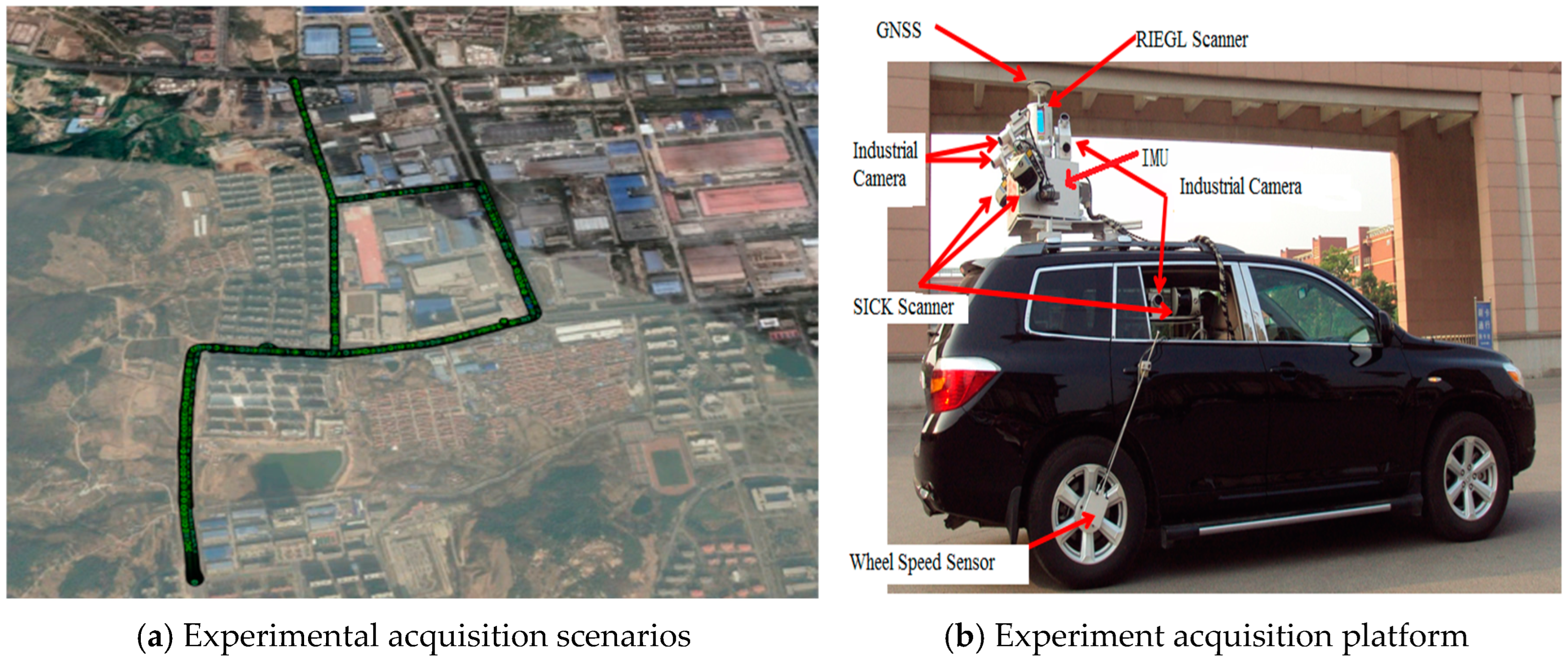
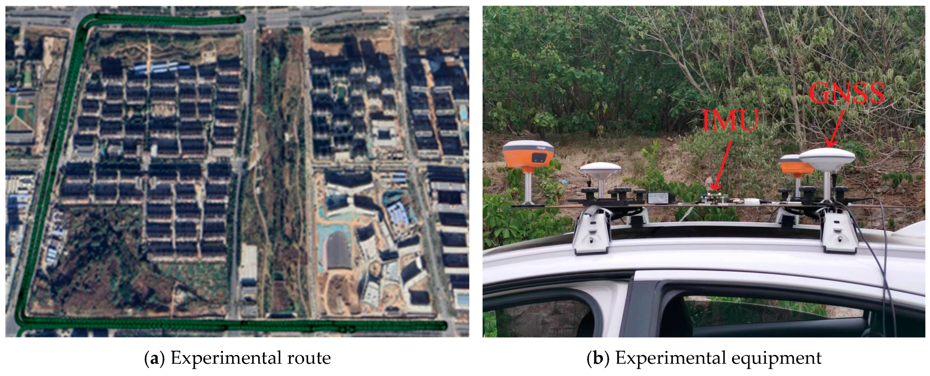
3.1. High-Precision Sensor On-Vehicle Experiment

The data collection site was located in Qingdao City and featured an open area with some buildings, resulting in partial occlusion. The experimental collection area is depicted in Figure 2a. The reference station for this dataset utilizes a Novatel ProPak6 receiver, which was installed on the roof of an open experimental building. The Novatel ProPak6 receiver and the SPAN-LCI fiber-optic inertial navigation system were mounted on a mobile measurement vehicle (Figure 2b). The GNSS receiver collects at a frequency of 1 Hz, while the IMU sampling frequency was 200 Hz. The total duration of the data collection was approximately 40 min. The specific parameters of IMU are shown in

Table 1. SPAN LCI inertial guidance nominal performance indicators.

Type of IMU		High-Precision IMU
Gyroscope Performance	Rate bias	<0.25°/h
	Angular random walk	<0.04°/$\surd \mathrm{h}$
Accelerometer Performance	Bias	<1 mg
	Random walk	<0.03 m/s/$\surd \mathrm{h}$
Collection Frequency		200 Hz

.

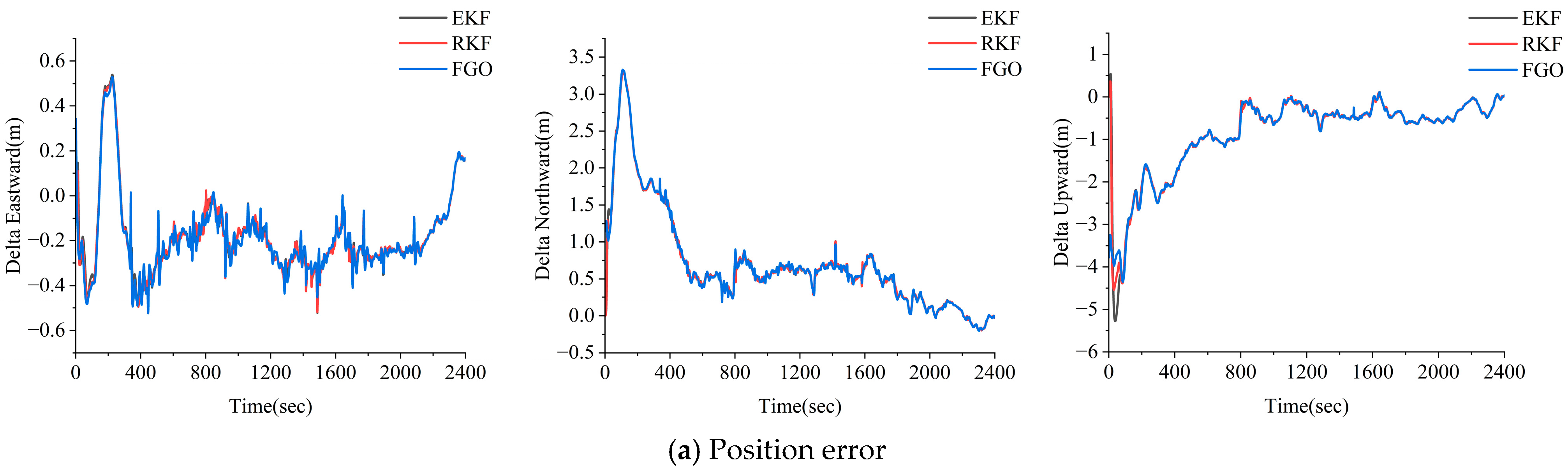
3.1.1. GNSS PPP/INS Combined Performance Analysis

In this paper, the combined navigation data collected by this group of high-precision sensors are solved using three GNSS PPP/INS loosely coupled models containing the EKF, RKF, and FGO models. Figure 3 presents the errors of the position, velocity, and attitude compared to the true values for the combined GNSS PPP/INS solutions of the three algorithms. In Figure 3a,b, in the initial stage, compared with the EKF and RKF methods, the GNSS PPP/INS combination based on FGO has better stability in terms of position and velocity, and the FGO algorithm produces lower error jumps in position and velocity estimation results. In Figure 3c, the combined FGO-based navigation attitude results are superior to those of the EKF and RKF models, especially in terms of the roll angle and heading angle.

To further compare the performance of the combined EKF, RKF, and FGO navigation parameter estimation methods, we statistically calculate the root mean square (RMS) values of the position, velocity, and attitude after convergence to 1 m in the east (E), north (N), and up (U) directions. The results are presented in

Table 2. Position, velocity, and attitude RMS values for three estimation methods of high precision inertial guidance.

ERROR		EKF	RKF	FGO
Position (m)	E	0.259	0.256	0.256
	N	0.507	0.507	0.506
	U	0.525	0.524	0.524
Velocity (m/s)	E	0.051	0.049	0.049
	N	0.045	0.043	0.043
	U	0.101	0.100	0.095
Attitude (deg)	Roll	0.010	0.009	0.006
	Pitch	0.021	0.017	0.015
	Heading	0.065	0.050	0.048

. Analysis of Table 2 reveals that due to the favorable environment of the survey area, the EKF, RKF, and FGO methods exhibit comparable position RMS values in the E, N, and U directions. The results of the FGO method are slightly superior to those of the EKF and RKF methods. In terms of velocity, the FGO method is 2.3%, 5.3%, and 5.6% more accurate than the EKF method in the E, N, and U directions, respectively. The FGO method is 5.1% more accurate than the RKF model in the U directions, respectively. The attitude accuracy of the FGO method is 40.3%, 27.3%, and 26.2% better than that of the EKF method in the traverse, pitch, and heading directions, respectively, and 31.1%, 8.4%, and 4.0% better than that of the RKF method in the traverse, pitch, and heading directions, respectively. The FGO method improves the terms of attitude better than the position and velocity.

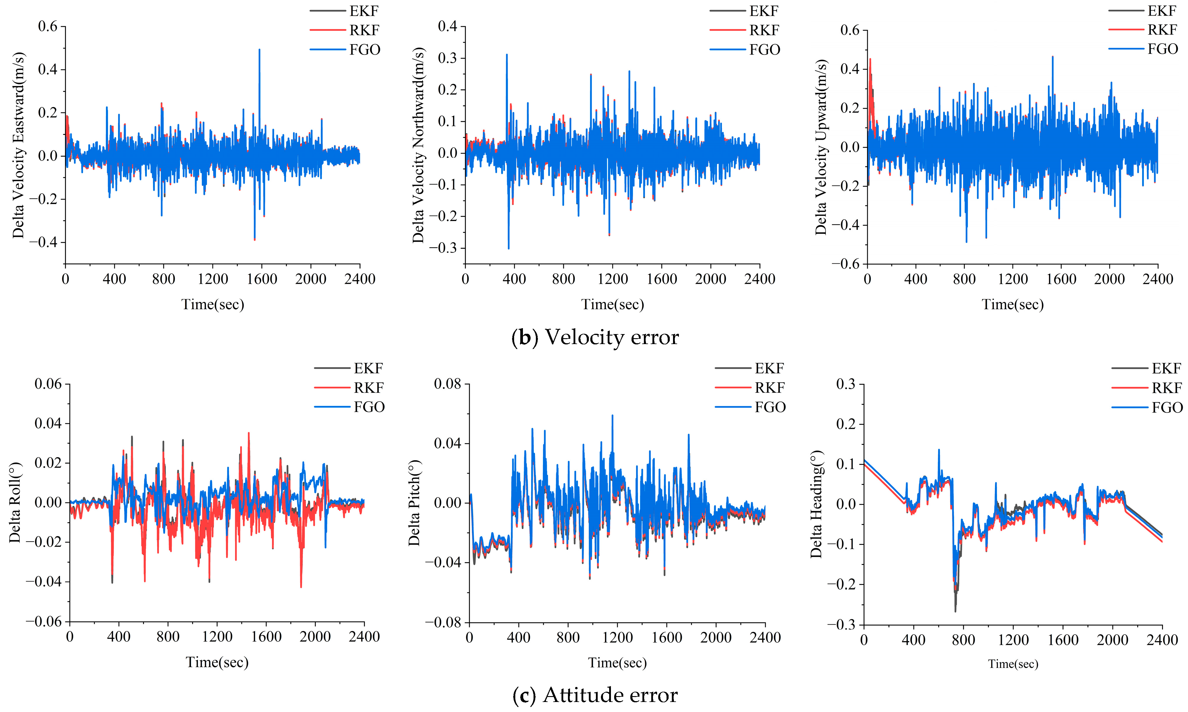
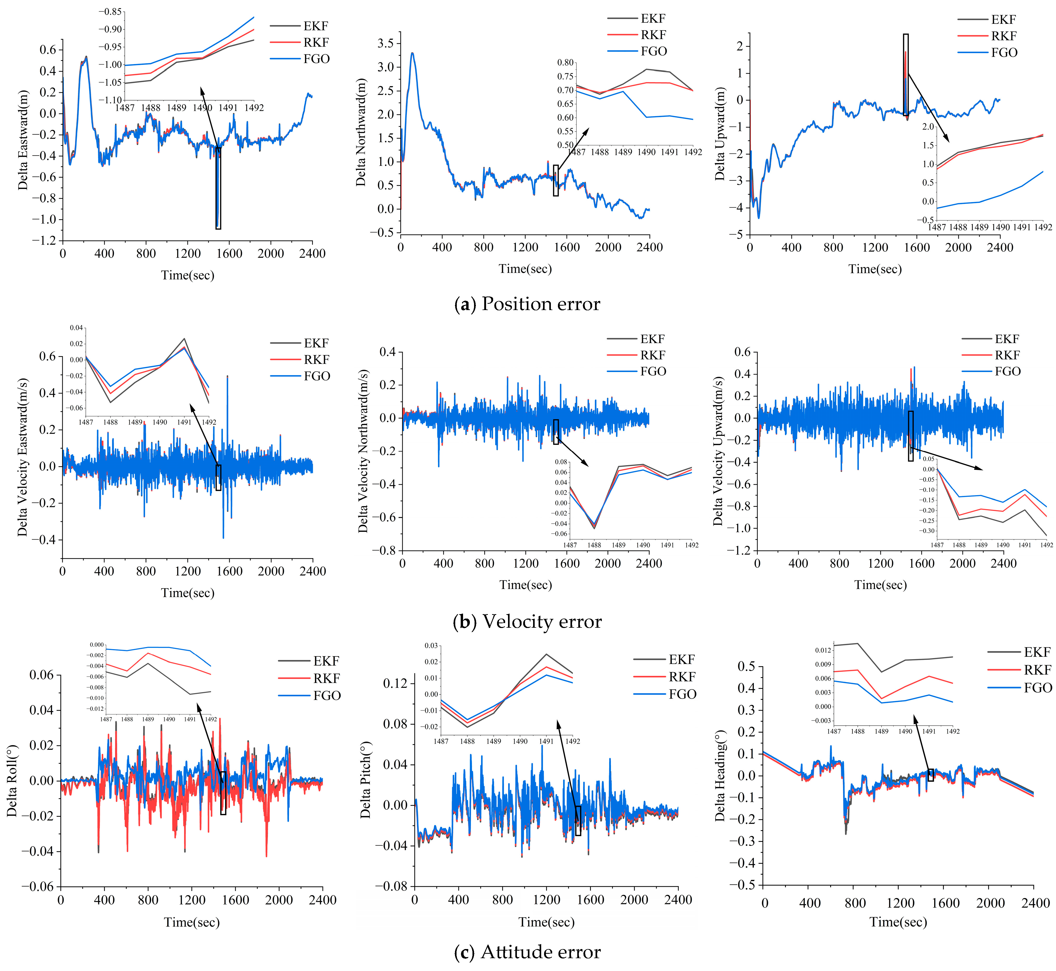
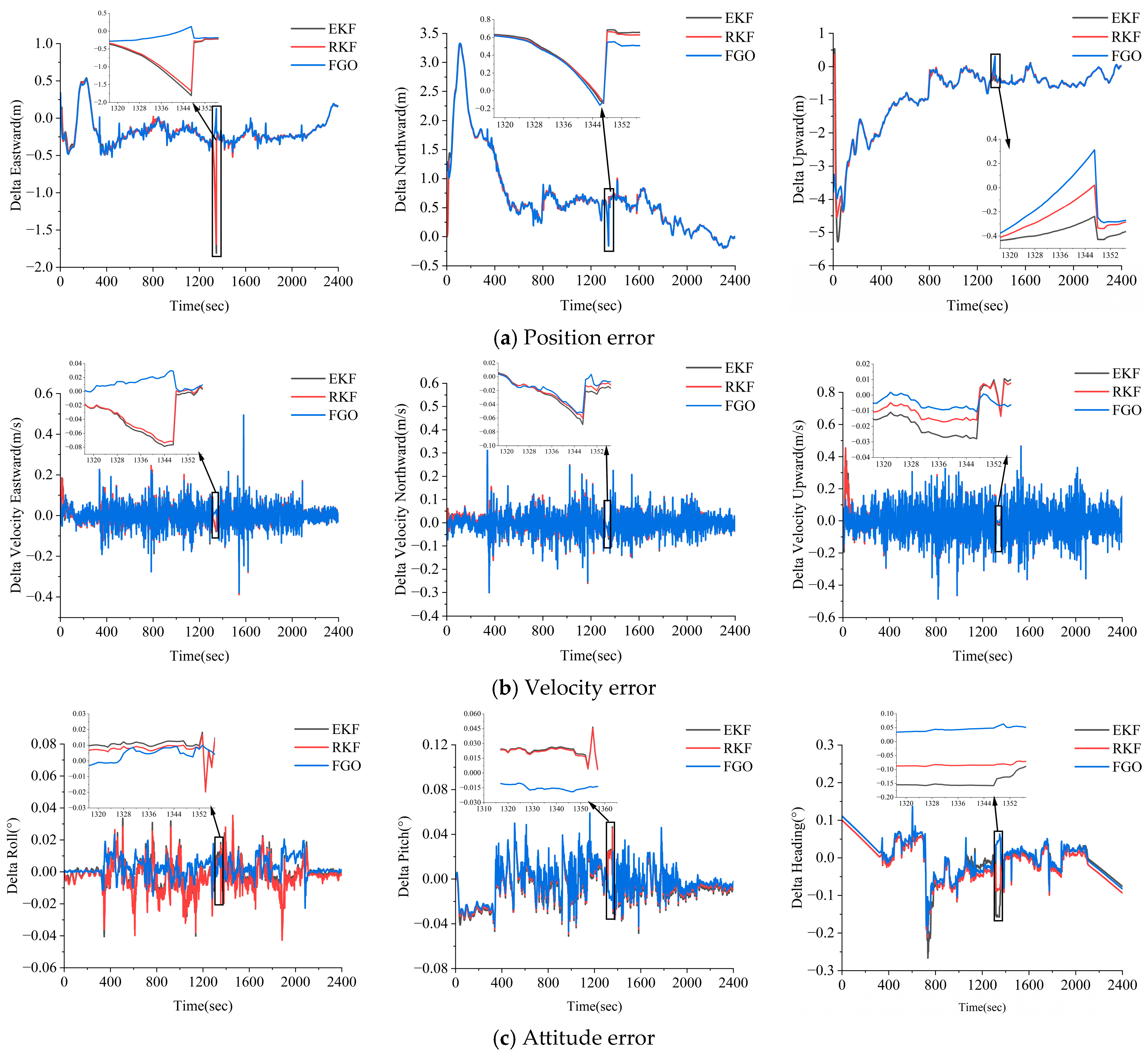
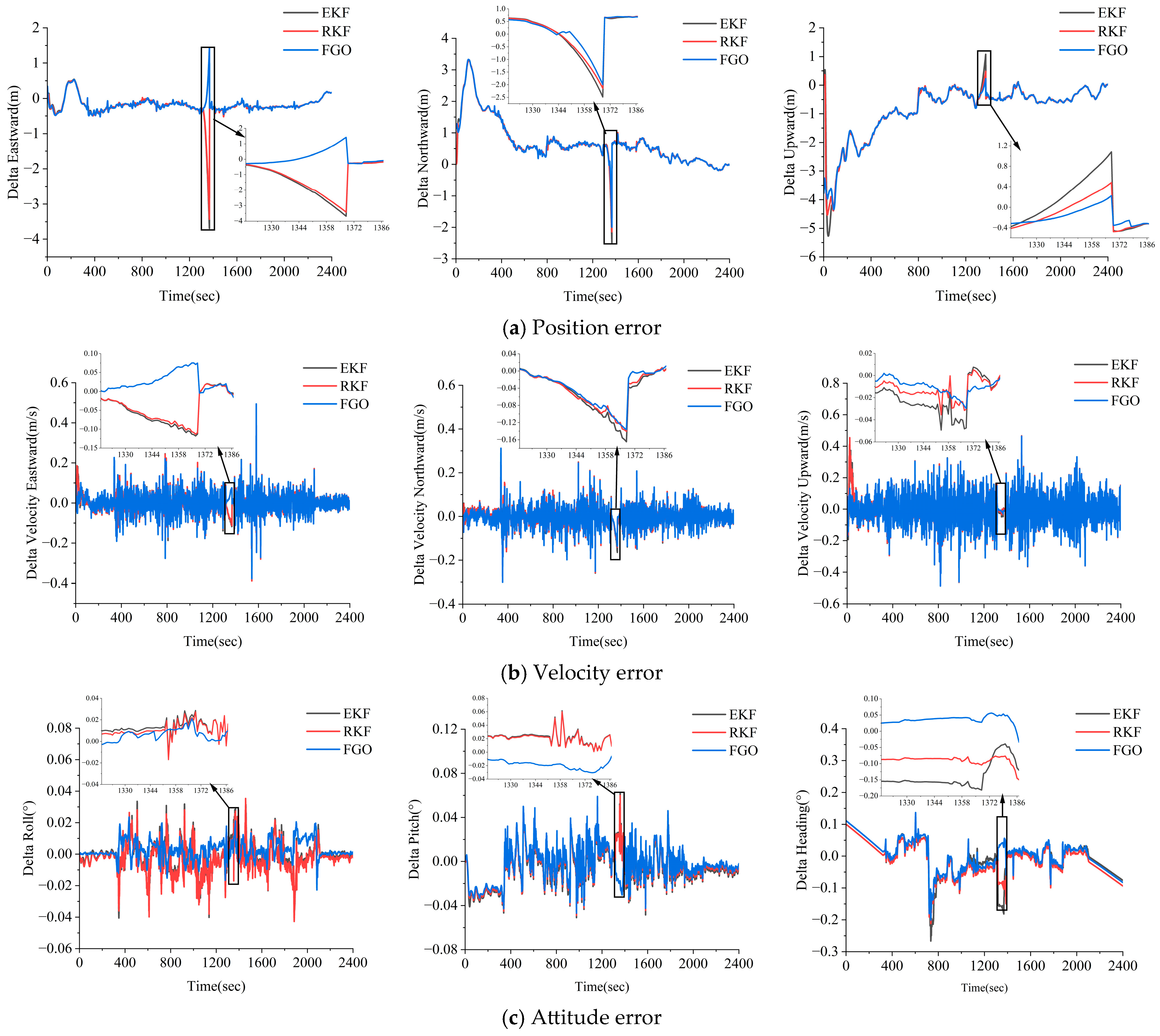
3.1.2. Simulated Gross GNSS PPP/INS Combined Navigation Performance Analysis

To further analyze the robustness of the FGO algorithm, this dataset was used to simulate the 5 s observing gross error in the GNSS PPP positioning results from epochs 1487 to 1492. For this dataset, the loosely coupled GNSS PPP/INS solutions are computed using the EKF, RKF, and FGO models. Figure 4 shows the errors in the position, velocity, and attitude of the GNSS PPP/INS combined solutions compared to the true values for the three algorithms. As shown in Figure 4a,b, due to the impact of the gross errors, the position and velocity errors for all three combined solutions exhibit significant fluctuations. The GNSS PPP/INS combined results based on the FGO parameter estimation method have superior position and velocity accuracies compared to the EKF and RKF parameter estimation methods. As shown in Figure 4c, the attitude of the combined system that uses the FGO method during the simulated gross error epochs is better than those that use the EKF and RKF methods.

Table 3. Simulated gross three parameter estimation methods for position, velocity, and attitude errors RMS values.

ERROR		EKF	RKF	FGO
Position (m)	E	0.993	0.977	0.954
	N	0.729	0.711	0.654
	U	1.476	1.418	0.383
Velocity (m/s)	E	0.035	0.027	0.021
	N	0.061	0.056	0.050
	U	0.232	0.181	0.131
Attitude (deg)	Roll	0.007	0.005	0.002
	Pitch	0.016	0.012	0.009
	Heading	0.011	0.006	0.003

presents the RMS error values for the position, velocity, and attitude during the simulated gross error epochs using the three parameter estimation methods. The FGO model improves the position accuracy by 3.9%, 11.4%, and 74.2% in the E, N, and U directions compared to the EKF model. The FGO model improves the accuracy by 2.3%, 9.3%, and 73.0% in the E, N, and U directions compared to the RKF model. Regarding the velocity, the FGO model achieves improvements of 39.6%, 17.9%, and 43.3% in the E, N, and U directions compared to the EKF model, and it achieves improvements of 22.5%, 10.4%, and 27.6% compared to the RKF model. Regarding the attitude, the FGO model yields accuracy improvements of 73.5% for the roll, 41.2% for the pitch, and 70.4% for the yaw compared to the EKF model, and it improves the accuracy by 55.0%, 22.9%, and 44.6% compared to the RKF model. This indicates that the FGO model achieves enhanced robustness against gross errors. Consequently, the FGO model yields superior estimates of the position, velocity, and attitude.

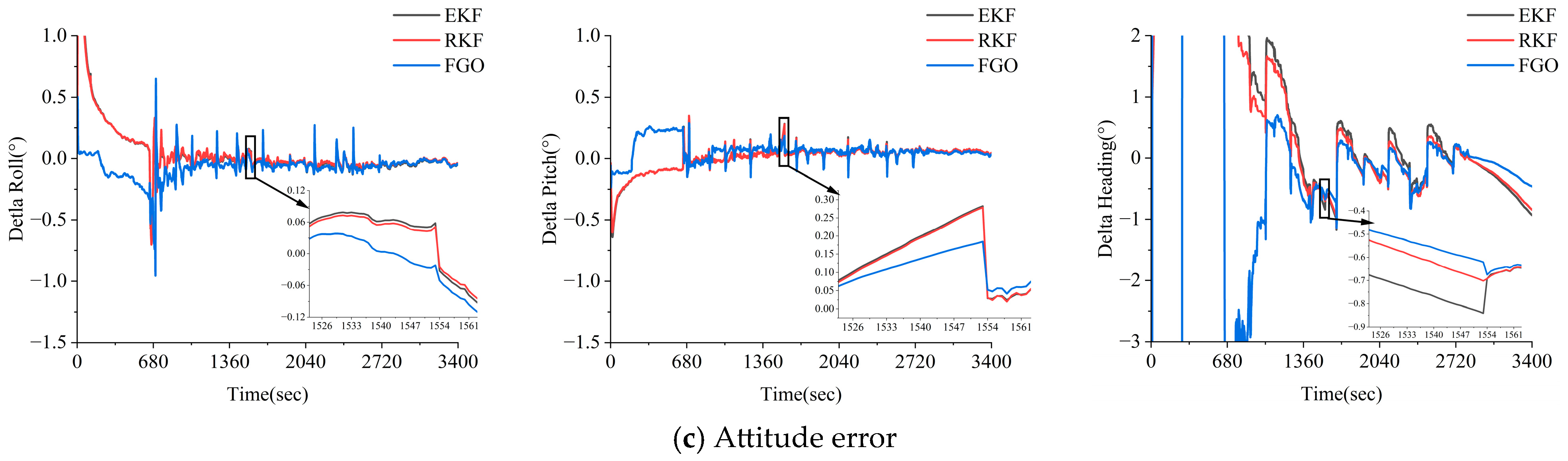
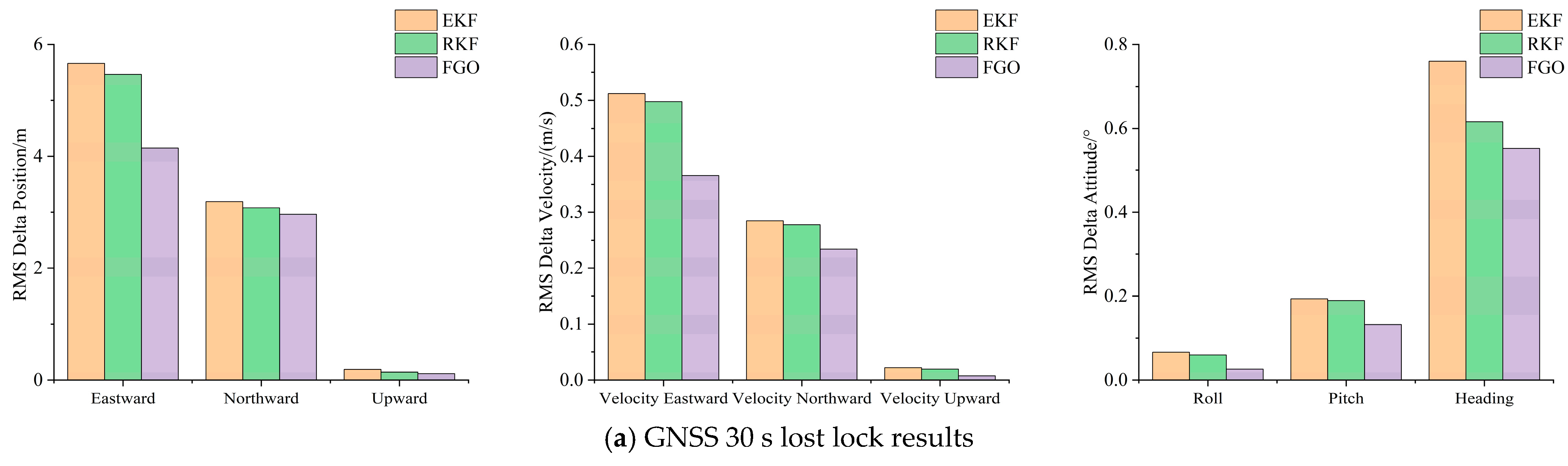
3.1.3. Performance Analysis of the GNSS PPP/INS Combination for Three Methods of GNSS Loss of Lock Scenarios

To further explore the performances of the EKF, RKF, and FGO model, in a GNSS signal rejection environment, the performance of the parameter estimations of the three methods is analyzed for simulated GNSS 30 s (1318–1348 epochs) and 60 s (1318–1368 epochs) loss-of-lock conditions. Figure 5 presents the GNSS loss-of-lock 30 s position, velocity, and attitude errors of the three GNSS PPP/INS methods. As can be seen from Figure 5a,b, during the time period when the GNSS signals are out of lock, for all three methods, the position and velocity have large cumulative errors. The full-time cumulative errors of the position and velocity based on the EKF method reach 1.038 m and 0.052 m/s. The RKF method slightly improves the accumulation of the errors. The FGO method more significantly improves the cumulative errors of the position and velocity, and it reduces the full-time cumulative 3-D position and velocity errors to 0.432 m and 0.027 m/s. As can be seen from Figure 5c, in terms of the attitude, the RKF method somewhat improves the accumulation of the errors compared to the EKF method. The cumulative 3-D position and velocity errors are reduced to 0.432 m and 0.027 m/s. As can be seen from Figure 5c, in terms of the attitude, to a certain extent, the RKF method improves the accuracy of the attitude compared to the EKF method. The FGO method yields optimal accuracy.

Figure 6 presents the position, velocity and attitude errors of the three methods GNSS PPP/INS for the GNSS loss-of-lock 60 s scenario. As can be seen from Figure 6a,b, during the time period when the GNSS signals are out of lock, the position and velocity of all three methods have large cumulative errors. For the EKF-based method, the full-time cumulative errors of the position and velocity reach 1.794 m and 0.072 m/s. The RKF method slightly improves the accumulation of the errors. The FGO method improves the cumulative errors of the position and velocity more significantly, with full-time cumulative 3-D position and velocity errors of 0.692 m and 0.061 m/s. As can be seen from Figure 6c, in terms of the attitude, to a certain extent, the RKF method improves the accuracy of the attitude compared to the EKF method, and the FGO method significantly improves the effect.

Figure 7 presents the RMS values of the position, velocity, and attitude errors for the three parameter estimation methods for both the 30 s (1318–1348 epochs) and 60 s (1318–1368 epochs) statistical GNSS loss-of-lock scenarios. In the 30 s GNSS loss-of-lock scenario, the FGO method improves the accuracy of the position by 81.1%, 3.9%, and 40.5% in the E, N, and U directions, respectively, compared to the EKF method, and the FGO method improves the positioning accuracy by 79.8%, 1.3%, and 14.9% in the E, N, and U directions, respectively, compared to the RKF method. The FGO method improves the accuracy of the velocity by 69.8%, 15.3%, and 69.6% in the E, N, and U directions, respectively, compared to the EKF method, and improves the accuracy of the velocity by 67.6%, 6.9%, and 49.2% in the E, N, and U directions, respectively, compared to the RKF method. Compared to the EKF method, the FGO method improves the accuracies of the roll, pitch, and heading angles by 50.0%, 38.4%, and 73.1%, respectively, and improves the accuracies of the roll, pitch, and heading angles by 32.9%, 35.5%, and 50.9%, respectively, compared to the RKF method. As regards the GNSS rejection for the 60 s scenario, the FGO method improves the accuracy of the position by 71.9%, 24.4%, and 53.8% in the N, E, and U directions, respectively, compared to the EKF method, and improves the accuracy by 69.9%, 15.0%, and 25.2% compared to the RKF method. The FGO method improves the accuracy of the velocity by 45.9%, 15.7%, and 52.8% in the E, N, and U directions, respectively, compared to the EKF method, and improves it by 41.9%, 6.2%, and 23.1% compared to the RKF method. The FGO method improves the accuracies of roll, pitch, and heading by 41.8%, 18.8% and 75.1%, respectively, compared to the EKF method, and improves the respective accuracies by 31.6%, 14.6%, and 56.7% compared to the RKF method. In summary, for the different GNSS loss-of-lock durations, the FGO method yields optimal results in terms of the position, velocity, and attitude compared to the EKF and RKF methods.

3.2. In-Vehicle Experiments with Consumer Grade Sensors

The data collection site of this set of data were located in Jinan City, and the collection area contained buildings and boulevard road shading. The experimental collection area is shown in Figure 8a. The Beiyun A1 consumer series GNSS/MEMS combination navigation board was mounted on a mobile survey vehicle (Figure 8b), and the IMU of this board was ADIS16505 (

Table 4. Consumer-grade IMU parameters.

Type of IMU		Consumer-Grade IMU
Gyroscope Performance	Rate bias	<2.7°/h
	Angular random walk	<0.2°/$\surd \mathrm{h}$
Accelerometer Performance	Bias	<2 mg
	Random walk	<0.3 m/s/$\surd \mathrm{h}$
Collection Frequency		100 Hz

). The GNSS data were sampled at a frequency of 1 Hz, and the IMU data were sampled at 100 Hz. The data collection period was approximately 50 min.

3.2.1. GNSS PPP/INS Combination Performance Analysis

Figure 9 presents the errors of the combined GNSS PPP/INS position, velocity, and attitude results obtained using the EKF, RKF, and FGO methods with respect to the reference truth values. Due to the fact that the vehicle made many sharp turns and U-turns during the data acquisition process, in Figure 9, the positions, velocities, and attitudes solved using the three methods exhibit jumps at the U-turns compared to the reference values. In terms of the position, the accuracies of the results obtained using the three methods are comparable, and all three directions converge within 0.5 m. In terms of the velocity, it can be seen that the FGO method converges most quickly during the initial static alignment phase. Furthermore, the attitude fluctuations estimated using the FGO method are significantly smaller than those estimated using the EKF and RKF methods, and the heading angles of the three methods fluctuate more in the alignment phase due to the use of consumer grade MEMS sensors.

Table 5. Combined system position, velocity, and attitude RMS values for the three methods.

ERROR		EKF	RKF	FGO
Position (m)	E	0.283	0.281	0.280
	N	0.132	0.116	0.114
	U	0.343	0.343	0.343
Velocity (m/s)	E	0.031	0.027	0.022
	N	0.131	0.108	0.020
	U	0.020	0.018	0.011
Attitude (deg)	Roll	0.162	0.158	0.119
	Pitch	0.103	0.101	0.095
	Heading	0.421	0.392	0.290

presents the statistics of the RMS values of the position, velocity, and attitude errors after convergence of the combined model containing the three methods. As can be seen from Table 5, in terms of the position, the accuracy of the FGO method is slightly better than those of the EKF and RKF methods due to the better environment of the survey area, in which the gross errors do not result in interference. The FGO method improves the accuracy of the velocity by 30.3%, 84.7%, and 45.4% in the E, N, and U directions, respectively, compared to the EKF method, and it improves the accuracy by 19.8%, 81.5%, and 39.2% in the three directions compared to the RKF method. In terms of the attitude, the FGO improves the accuracy by 26.6%, 7.3%, and 31.1% in the traverse, pitch, and heading directions, respectively, compared to the EKF method, and it improves the accuracy by 24.8%, 5.4%, and 26.1% in the three directions compared to the RKF method.

3.2.2. Simulated Gross GNSS PPP/INS Combined Navigation Performance Analysis

To further analyze the robustness of the EKF, RKF, and FGO methods we continuously introduced errors from epochs 1904–1908. Figure 10 presents the GNSS PPP/INS position, velocity, and attitude errors of the three methods. As can be seen from Figure 10, due to the introduction of gross errors, all three methods exhibit fluctuations in the position, velocity, and attitude. The FGO method yields smaller errors regarding the position, velocity, and attitude than the EKF and RKF methods do.

Table 6. Presents the RMS statistics of position, velocity, and attitude errors for the combined systems of the three methods under simulated gross errors.

ERROR		EKF	RKF	FGO
Position (m)	E	0.337	0.317	0.286
	N	0.190	0.159	0.121
	U	0.522	0.458	0.403
Velocity (m/s)	E	0.186	0.174	0.049
	N	0.127	0.106	0.080
	U	0.372	0.303	0.102
Attitude (deg)	Roll	0.100	0.085	0.072
	Pitch	0.140	0.112	0.067
	Heading	0.392	0.317	0.148

presents the RMS values of the position, velocity, and attitude errors in three directions during the time periods in which gross errors are introduced. An analysis of Table 6 reveals that in terms of position, in the E, N, and U directions, the FGO method improves the accuracy by 15.2%, 36.4%, and 22.8% compared to the EKF method, and it improves the accuracy by 9.9%, 24.1%, and 11.9% compared to the RKF method. In terms of the velocity, in the E, N, and U directions, the FGO method improves the accuracy by 73.8%, 37.3%, and 72.9% compared to the EKF method, and it improves the accuracy by 72.1%, 24.7%, and 66.7% compared to the RKF method. In terms of the attitude, the FGO improves the accuracy by 28.4%, 52.3%, and 62.3% in the traverse, pitch, and heading directions compared to the EKF method, and it improves the accuracy by 15.1%, 40.3%, and 53.3% compared to the RKF method.

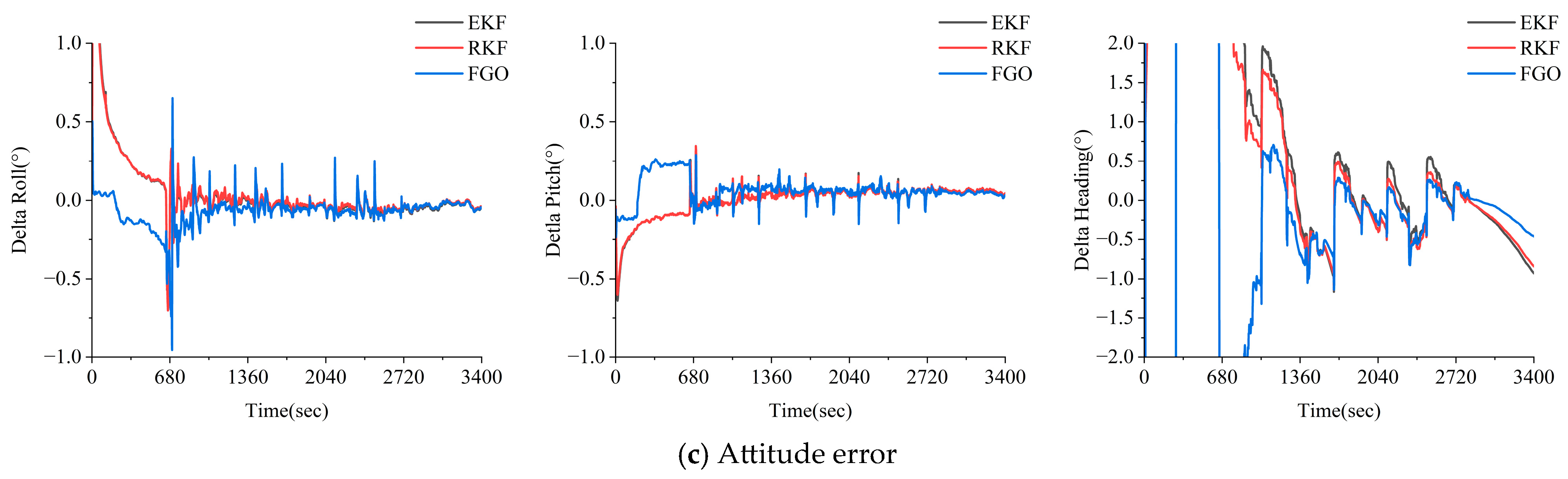
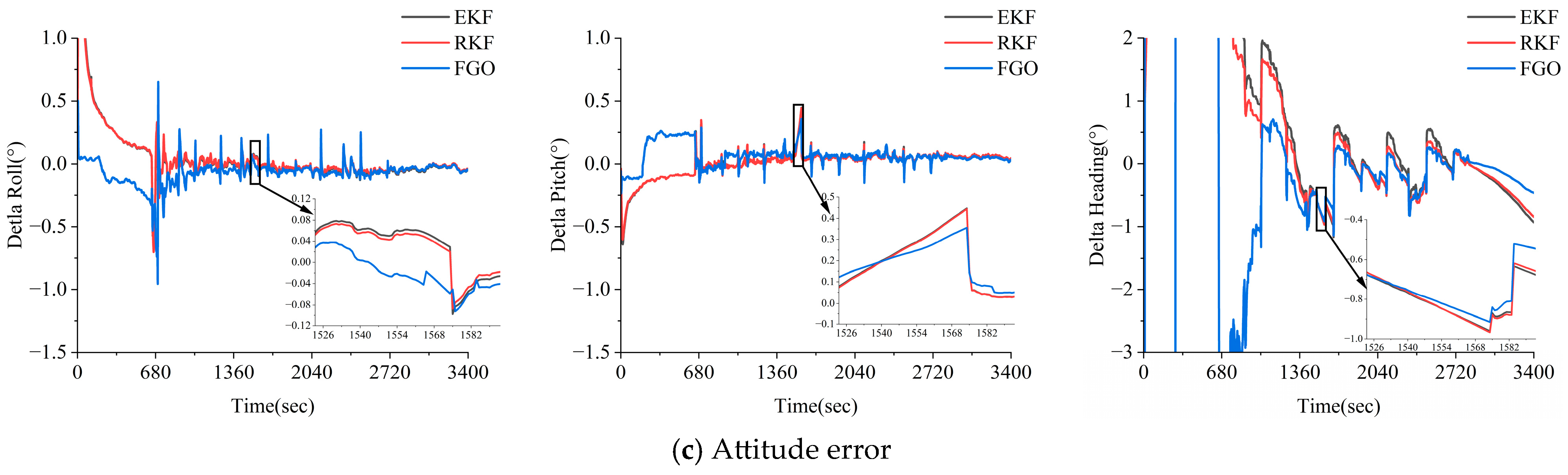
3.2.3. Analysis of GNSS PPP/INS Combined Performance Under GNSS Loss-of-Lock Conditions

To further explore the performances of the EKF, RKF and FGO method, in a GNSS signal rejection environment, the parameter estimation performances of these three methods are analyzed for the simulated GNSS 30 s and 60 s loss-of-lock scenarios. Figure 11 and Figure 12 present the GNSS/INS position, velocity, and attitude errors of the three combined models for the 30 s and 60 s scenarios. As can be seen from Figure 11a,b, for all three methods, the position and velocity have large cumulative errors during the time period of the GNSS signal loss, The full-time cumulative errors of the position and velocity reach 5.660 m and 0.512 m/s for the EKF method. The RKF method slightly improves the accumulation of the errors, and the FGO method is able to improve the cumulative errors of the position and velocity more significantly. It reduces the full-time cumulative 3-D position and velocity errors to 4.151 m and 0.366 m/s. As can be seen from Figure 11c, for all three methods, the attitude results exhibit jumps due to the absence of GNSS, and the attitude errors of the FGO method are smaller compared to those of the EKF and RKF methods.

Figure 12 presents the GNSS PPP/INS position, velocity, and attitude errors of the three methods for the GNSS loss-of-lock 60 s scenario. As can be seen from Figure 12a,b, during the GNSS signals out-of-lock time period, for all three methods, the position and velocity have large cumulative errors, the full-time cumulative errors of the EKF method reach 17.739 m and 1.027 m/s for the position and velocity, the RKF method slightly improves the accumulation of the errors, and the FGO method improves the cumulative errors of the position and velocity more significantly. For the FGO method, the maximum three-dimensional position and velocity errors are reduced to 12.529 m and 0.709 m/s. As can be seen from Figure 12c, for all three methods, there is no error accumulation for the attitude. The RKF method improves the accuracy of the attitude to some extent, and the FGO method improves it significantly.

Figure 13 presents the RMS statistics of the position, velocity, and attitude errors of the system for the three methods combined during the GNSS loss-of-lock time period. As can be seen from Figure 13, in the GNSS loss-of-lock 30 s scenario, the FGO method improves the accuracy of the position by 26.6%, 7.2%, and 39.2% in the E, N, and U directions compared to the EKF method, and it improves the accuracy by 23.9%, 3.8%, and 18.2% in the E, N, and U directions compared to the RKF method. In terms of the velocity, the FGO improves the accuracy by 28.6%, 17.9%, and 65.6% in the E, N, and U directions compared to the EKF method, and the FGO improves the accuracy by 26.6%, 15.8%, and 60.7% in the E, N, and U compared to the RKF method. In terms of attitude, the FGO accuracy is improved by 61.2%, 31.6%, and 27.3% in the roll, pitch, and heading directions compared to the EKF method, and the FGO accuracy is improved by 57.1%, 30.1%, and 10.3% compared to the RKF method. In the case of GNSS out-of-lock for 60 s, in terms of position, the FGO method accuracy is improved by 29.4%, 22.1%, and 13.5% in the E, N, and U directions compared to the EKF method, and the FGO method improves the accuracy by 27.6%, 20.5%, and 4.1% compared to the RKF method. In terms of the velocity, the FGO method improves the accuracy by 31.0%, 28.9%, and 44.8% in the E, N, and U directions compared to the EKF method, and the FGO method improves the accuracy by 29.7%, 28.1%, and 42.7% compared to the RKF method. In terms of the attitude, the FGO method improves the accuracy by 37.8%, 12.4%, and 3.2% in the roll, pitch, and heading directions, compared to the EKF method, and the FGO accuracy improves the accuracy by 30.0%, 11.3%, and 3.1% compared to the RKF method.

In summary, for the urban scene data collected using both high and low precision GNSS/INS, the position, velocity, and attitude results of the combined system based on the FGO method are better than those of the conventional EKF and RKF methods. For the simulated conditions affected by coarse errors, the parameter estimation results of the FGO method are optimal and those of the RKF method are the second best. For the simulated conditions with different time periods of GNSS lock of loss, the FGO method yields best parameter estimation results, followed by the RKF method, and the EKF method yields the worst results.

4. Conclusions

Observations are susceptible to gross interference and frequent signal interruptions, resulting in the inability of the combined GNSS/INS system to obtain reliable and highly accurate positioning and centering results in urban environments. To this end, in this study, we investigated a combined GNSS/INS model based on the FGO method, and we analyzed the robust performance of the FGO method in urban occluded scenes. We used a vehicle mounted system using high and low precision inertial guidance to collect dynamic data of urban scenes for experimental analysis. The following conclusions were drawn.

(1)

Compared to the EKF and RKF methods, the FGO strategy has a good anti-discrepancy effect and stability. The FGO method utilizes IMU factors and GNSS factors to construct a sliding window solution, which can better utilize the constraints between the calendar elements within the window and the redundant observation information to suppress the effect of the coarseness.

(2)

In the simulated gross errors experiments, the FGO method yielded a better resistance to errors compared to the EKF and RKF methods. In the high-precision inertial guidance experiments, the FGO model yielded maximum improvements of 74.2% and 73.0% in the positions, 43.3% and 27.6% in the velocity, and 73.5% and 55.0% in the attitude compared to the EKF and RKF models. In the consumer grade inertial guidance experiments, the FGO model yielded maximum improvements of 36.4% and 24.1% in the position, the maximum improvements of 73.8% and 72.1% in the velocity, and = maximum improvement of 62.3% and 53.3% in the attitude.

(3)

In the simulated GNSS loss experiments, the GNSS/INS integration system based on the FGO method yielded a higher parameter estimation accuracy. In the high-precision inertial guidance experiments, the FGO model yielded maximum improvements of 81.1% and 79.8% in the position, 69.8% and 67.6% in the velocity, and 75.1% and 56.7% in the attitude compared to the EKF and RKF models, and the FGO model yielded maximum improvements of 39.2% and 27.6% in the position, 65.6% and 60.7% in the velocity, and 61.2% and 57.1% in the attitude compared to the EKF and RKF models. In the consumer grade inertial guidance experiments, the FGO model yielded maximum improvements of 65.6% and 60.7% in the velocity and maximum improvements of 61.2% and 57.1% in the attitude.

In the context of combined GNSS/INS navigation, particularly for in-vehicle systems operating in urban environments, the FGO method stands out as a superior technique compared to traditional filtering methods like the EKF and the RKF. This superiority is most evident in its enhanced tolerance to measurement noise and dynamic changes, which are common in urban settings where signal obstructions, multipath errors, and rapid changes in vehicle dynamics are frequent. The results of this study provide a theoretical reference and practical support for intelligent driving in urban scenarios.

References

1. Pan, L.; Zhang, X.; Liu, J.; Li, X.; Li, X. Performance Evaluation of Single-frequency Precise Point Positioning with GPS, GLONASS, BeiDou and Galileo. J. Navig. 2017, 70, 465–482. [Google Scholar] [CrossRef]
2. Zhang, X.; Zhang, Y.; Zhu, F.J.G. Factor graph optimization for urban environment GNSS positioning and robust performance analysis. Geomat. Inf. Sci. Wuhan Univ. 2023, 48, 1050–1057. [Google Scholar]
3. Zhang, X.; Tao, X.; Wang, Y.; Liu, W.; Zhu, F.J.G. MEMS-Enhanced Smartphone GNSS High-Precision Positioning for Vehicular Navigation in Urban Conditions. Geomat. Inf. Sci. Wuhan Univ. 2022, 47, 1740–1749. [Google Scholar]
4. Wang, D.; Dong, Y.; Li, Z.; Li, Q.; Wu, J. Constrained MEMS-based GNSS/INS tightly coupled system with robust Kalman filter for accurate land vehicular navigation. IEEE Trans. Instrum. Meas. 2019, 69, 5138–5148. [Google Scholar] [CrossRef]
5. Shi, B.; Wang, M.; Wang, Y.; Bai, Y.; Lin, K.; Yang, F. Effect analysis of GNSS/INS processing strategy for sufficient utilization of urban environment observations. Sensors 2021, 21, 620. [Google Scholar] [CrossRef] [PubMed]
6. Takasu, T.; Yasuda, A. Development of the low-cost RTK-GPS receiver with an open source program package RTKLIB. In Proceedings of the International Symposium on GPS/GNSS, Seoul, Republic of Korea, 1–3 December 2009. [Google Scholar]
7. Chai, D.; Chen, G.; Wang, S.J. A Novel Method of Adaptive Kalman Filter for Heading Estimation Based on an Autoregressive Model. Appl. Sci. 2019, 9, 3727. [Google Scholar] [CrossRef]
8. Hajiyev, C.; Soken, H.E. Robust adaptive Kalman filter for estimation of UAV dynamics in the presence of sensor/actuator faults. Aerosp. Sci. Technol. 2013, 28, 376–383. [Google Scholar] [CrossRef]
9. Gao, W.; Li, J. Adaptive Kalman filtering for the integrated SINS/DVL system. J. Comput. Inf. Syst. 2013, 9, 6443–6450. [Google Scholar]
10. Sage, A.P.; Husa, G.W. Adaptive filtering with unknown prior statistics. In Proceedings of the Joint Automatic Control Conference, Boulder, CO, USA, 12–15 August 1969. [Google Scholar]
11. Ma, L.; Li, X. Improved Algorithmof Adaptive Fading Kalman Filtering Based on GPS/INS Integrated Navigation. Sci. Technol. Eng 2013, 13, 9973–9977. [Google Scholar]
12. Godha, S.; Cannon, M. GPS/MEMS INS integrated system for navigation in urban areas. GPS Solut. 2007, 11, 193–203. [Google Scholar] [CrossRef]
13. Huber, P.J. Robust estimation of a location parameter. In Breakthroughs in Statistics: Methodology and Distribution; Springer: Berlin/Heidelberg, Germany, 1992; pp. 492–518. [Google Scholar]
14. Yang, Y.; Gao, W.-G.; Zhang, X.-D. Robust Kalman filtering with constraints: A case study for integrated navigation. J. Geod. 2010, 84, 373–381. [Google Scholar] [CrossRef]
15. Gao, S.; Zhong, Y.; Li, W. Robust adaptive filtering method for SINS/SAR integrated navigation system. Aerosp. Sci. Technol. 2011, 15, 425–430. [Google Scholar] [CrossRef]
16. Guo, Y.; Li, X.; Meng, Q. A runs test-based Kalman filter with both adaptability and robustness with application to INS/GNSS integration. IEEE Sens. J. 2022, 22, 22919–22930. [Google Scholar] [CrossRef]
17. Yin, Z.; Yang, J.; Ma, Y.; Wang, S.; Chai, D.; Cui, H.J.R.S. A Robust Adaptive Extended Kalman Filter Based on an Improved Measurement Noise Covariance Matrix for the Monitoring and Isolation of Abnormal Disturbances in GNSS/INS Vehicle Navigation. Remote Sens. 2023, 15, 4125. [Google Scholar] [CrossRef]
18. Watson, R.M.; Gross, J.N. Robust navigation in GNSS degraded environment using graph optimization. In Proceedings of the 30th International Technical Meeting of the Satellite Division of the Institute of Navigation (ION GNSS+ 2017), Portland, OR, USA, 25–29 September 2017. [Google Scholar]
19. Kschischang, F.R.; Frey, B.J.; Loeliger, H.-A. Factor graphs and the sum-product algorithm. IEEE Trans. Inf. Theory 2001, 47, 498–519. [Google Scholar] [CrossRef]
20. Dellaert, F.; Kaess, M. Square Root SAM: Simultaneous localization and mapping via square root information smoothing. Int. J. Robot. Res. 2006, 25, 1181–1203. [Google Scholar] [CrossRef]
21. Jinke, W.; Xingxing, Z.; Xiangrui, Z.; Jiajun, L.; Yong, L. Review of multi-source fusion SLAM: Current status and challenges. J. Image Graph. 2022, 27, 368–389. [Google Scholar]
22. Suzuki, T. First place award winner of the smartphone decimeter challenge: Global optimization of position and velocity by factor graph optimization. In Proceedings of the 34th International Technical Meeting of the Satellite Division of The Institute of Navigation (ION GNSS+ 2021), Nashville, TN, USA, 20–24 September 2021. [Google Scholar]
23. Suzuki, T. 1st place winner of the smartphone decimeter challenge: Two-step optimization of velocity and position using smartphone’s carrier phase observations. In Proceedings of the 35th International Technical Meeting of the Satellite Division of The Institute of Navigation (ION GNSS+ 2022), Denver, CO, USA, 19–23 September 2022. [Google Scholar]
24. Xin, S.; Wang, X.; Zhang, J.; Zhou, K.; Chen, Y. A Comparative Study of Factor Graph Optimization-Based and Extended Kalman Filter-Based PPP-B2b/INS Integrated Navigation. Remote Sens. 2023, 15, 5144. [Google Scholar] [CrossRef]
25. Zhang, Y.; Zhu, F.; Zhang, X. Improving Gnss Positioning Reliability and Accuracy Based on Factor Graph Optimization in Urban Environment. Int. Arch. Photogramm. Remote Sens. Spat. Inf. Sci. 2023, 48, 1179–1184. [Google Scholar] [CrossRef]
26. Wen, W.; Pfeifer, T.; Bai, X.; Hsu, L.T. Factor graph optimization for GNSS/INS integration: A comparison with the extended Kalman filter. Navigation 2021, 68, 315–331. [Google Scholar] [CrossRef]
27. Li, Z.; Lee, P.-H.; Hung, T.H.M.; Zhang, G.; Hsu, L.-T. Intelligent Environment-Adaptive GNSS/INS Integrated Positioning with Factor Graph Optimization. Remote Sens. 2023, 16, 181. [Google Scholar] [CrossRef]
28. Hu, Y.; Li, H.; Liu, W. Robust factor graph optimisation method for shipborne GNSS/INS integrated navigation system. IET Radar Sonar Navig. 2024, 18, 782–798. [Google Scholar] [CrossRef]
29. Zhang, L.; Tang, C.; Zhang, Y.; Song, H. Inertial-Navigation-Aided Single-Satellite Highly Dynamic Positioning Algorithm. Sensors 2019, 19, 4196. [Google Scholar] [CrossRef] [PubMed]
30. Wen, W.; Kan, Y.C.; Hsu, L.-T. Performance comparison of GNSS/INS integrations based on EKF and factor graph optimization. In Proceedings of the 32nd International Technical Meeting of the Satellite Division of The Institute of Navigation (ION GNSS+ 2019), Miami, FL, USA, 16–20 September 2019. [Google Scholar]
31. Mao, Y.; Sun, R.; Wang, J.; Cheng, Q.; Kiong, L.C.; Ochieng, W.Y. New time-differenced carrier phase approach to GNSS/INS integration. GPS Solut. 2022, 26, 122. [Google Scholar] [CrossRef]
32. Barfoot, T.D. State Estimation for Robotics; Cambridge University Press: Cambridge, UK, 2024. [Google Scholar]
33. Kaess, M.; Johannsson, H.; Roberts, R.; Ila, V.; Leonard, J.J.; Dellaert, F. iSAM2: Incremental smoothing and mapping using the Bayes tree. Int. J. Robot. Res. 2012, 31, 216–235. [Google Scholar] [CrossRef]
34. Zhang, S.; Tu, R.; Gao, Z.; Zou, D.; Wang, S.; Lu, X. LEO-Enhanced GNSS/INS Tightly Coupled Integration Based on Factor Graph Optimization in the Urban Environment. Remote Sens. 2024, 16, 1782. [Google Scholar] [CrossRef]
35. Tang, H.; Zhang, T.; Niu, X.; Fan, J.; Liu, J. Impact of the earth rotation compensation on MEMS-IMU preintegration of factor graph optimization. IEEE Sens. J. 2022, 22, 17194–17204. [Google Scholar] [CrossRef]
Figure 1. Loosely coupled PPP/INS model based on factor graph.
Electronics 14 00660 g001
Figure 2. Experiment acquisition scenario and platform.
Electronics 14 00660 g002
Figure 3. Position, velocity, and attitude errors of three estimation methods for high precision inertial guidance.
Electronics 14 00660 g003aElectronics 14 00660 g003b
Figure 4. Simulated gross three parameter estimation methods position, velocity, and attitude errors.
Electronics 14 00660 g004
Figure 5. Position, velocity, and attitude errors estimated by the three methods of the GNSS lost lock 30 s scenario.
Electronics 14 00660 g005
Figure 6. Position, velocity, and attitude errors estimated by the three methods in the GNSS lost lock 60 s scenario.
Electronics 14 00660 g006
Figure 7. Error position velocity attitude RMS values for different GNSS lost lock conditions.
Electronics 14 00660 g007
Figure 8. Experiment area and experiment acquisition platform.
Electronics 14 00660 g008
Figure 9. Consumer inertial guidance three methods of combining model position, velocity, and attitude errors.
Electronics 14 00660 g009aElectronics 14 00660 g009b
Figure 10. The position, velocity, and attitude errors of the three parameter estimation methods under simulated gross errors.
Electronics 14 00660 g010
Figure 11. GNSS loss of lock for 30 s three methods to combine system position, velocity, and attitude errors.
Electronics 14 00660 g011aElectronics 14 00660 g011b
Figure 12. GNSS loss of lock for 60 s three methods to combine system position, velocity, and attitude errors.
Electronics 14 00660 g012aElectronics 14 00660 g012b
Figure 13. GNSS error position, velocity and attitude RMS statistics for three methods with different loss-of-lock durations.
Electronics 14 00660 g013aElectronics 14 00660 g013b