
End-to-End Speech Recognition with Deep Fusion: Leveraging External Language Models for Low-Resource Scenarios

Abstract
:1. Introduction
2. Basic Theory
2.1. Zipformer
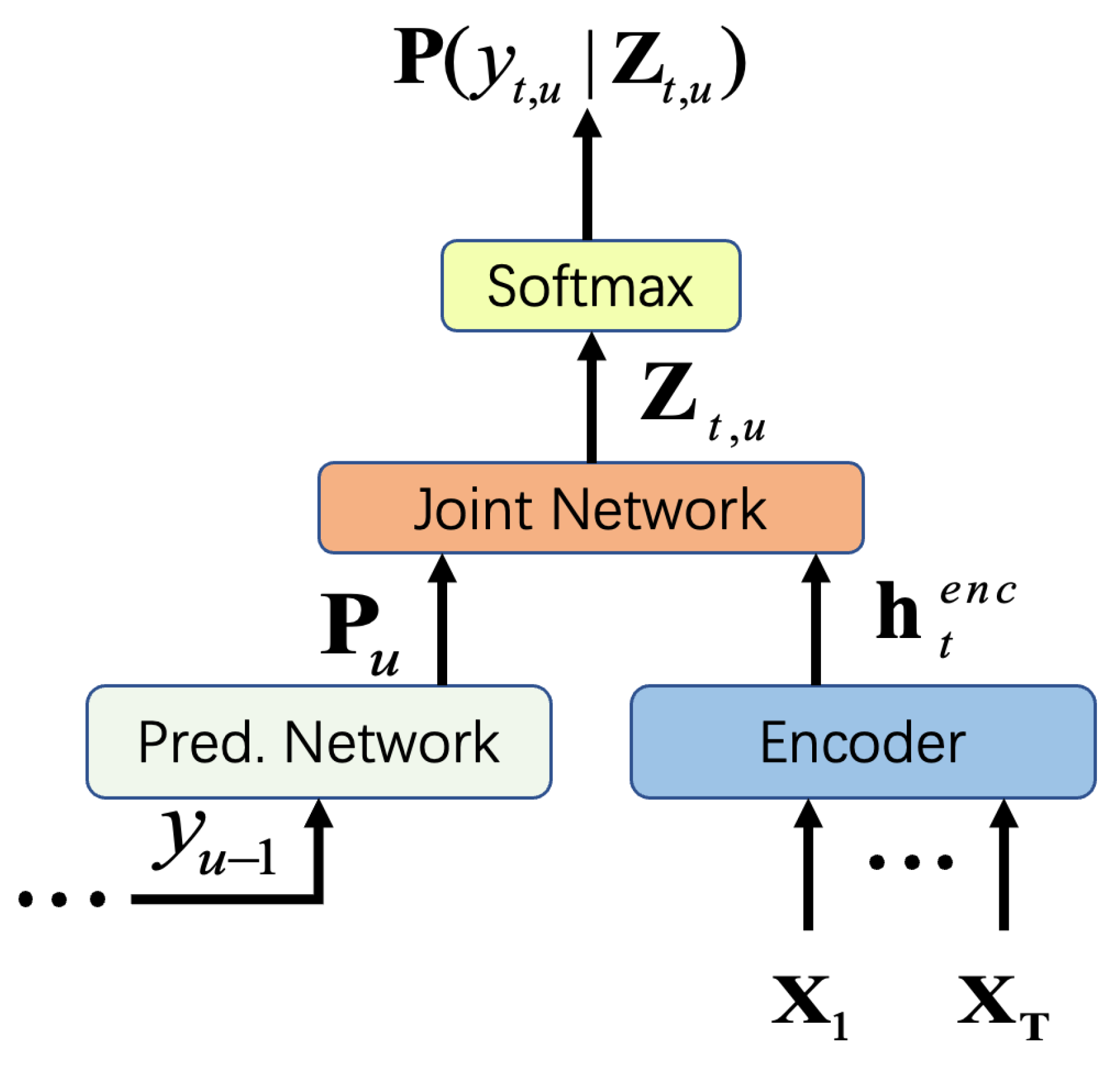
2.2. RNN-T
2.3. LM and Decoding Strategies
3. Training Process
3.1. Dataset and Preprocessing
3.2. Training Configuration
3.3. Deep Fusion
3.4. Loss Function
3.5. Evaluation Metrics
4. Results Comparison and Analysis
4.1. Main Results
4.2. Impact of Data Scale Differences
4.3. Performance Improvement from LM Fusion
4.4. Ablation Study
5. Conclusions
Author Contributions
Funding
Data Availability Statement
Conflicts of Interest
References
- Dhanjal, A.S.; Singh, W. A comprehensive survey on automatic speech recognition using neural networks. Multimed. Tools Appl. 2024, 83, 23367–23412. [Google Scholar] [CrossRef]
- Lakomkin, E.; Wu, C.; Fathullah, Y.; Kalinli, O.; Seltzer, M.L.; Fuegen, C. End-to-end speech recognition contextualization with large language models. In Proceedings of the ICASSP 2024—2024 IEEE International Conference on Acoustics, Speech and Signal Processing (ICASSP), Seoul, Republic of Korea, 14–19 April 2024; pp. 12406–12410. [Google Scholar]
- Ardila, R.; Branson, M.; Davis, K.; Henretty, M.; Kohler, M.; Meyer, J.; Morais, R.; Saunders, L.; Tyers, F.M.; Weber, G. Common voice: A massively-multilingual speech corpus. arXiv 2019, arXiv:1912.06670. [Google Scholar]
- Chen, G.; Chai, S.; Wang, G.; Du, J.; Zhang, W.-Q.; Weng, C.; Su, D.; Povey, D.; Trmal, J.; Zhang, J. Gigaspeech: An evolving, multi-domain asr corpus with 10,000 hours of transcribed audio. arXiv 2021, arXiv:2106.06909. [Google Scholar]
- Kang, W.; Yang, X.; Yao, Z.; Kuang, F.; Yang, Y.; Guo, L.; Lin, L.; Povey, D. Libriheavy: A 50,000 hours asr corpus with punctuation casing and context. In Proceedings of the ICASSP 2024—2024 IEEE International Conference on Acoustics, Speech and Signal Processing (ICASSP), Seoul, Republic of Korea, 14–19 April 2024; pp. 10991–10995. [Google Scholar]
- San, N.; Paraskevopoulos, G.; Arora, A.; He, X.; Kaur, P.; Adams, O.; Jurafsky, D. Predicting positive transfer for improved low-resource speech recognition using acoustic pseudo-tokens. arXiv 2024, arXiv:2402.02302. [Google Scholar]
- Ragni, A.; Knill, K.M.; Rath, S.P.; Gales, M.J. Data augmentation for low resource languages. In Proceedings of the INTERSPEECH 2014: 15th Annual Conference of the International Speech Communication Association, Singapore, 14–18 September 2014; pp. 810–814. [Google Scholar]
- Tu, T.; Chen, Y.-J.; Yeh, C.-c.; Lee, H.-Y. End-to-end text-to-speech for low-resource languages by cross-lingual transfer learning. arXiv 2019, arXiv:1904.06508. [Google Scholar]
- Byambadorj, Z.; Nishimura, R.; Ayush, A.; Ohta, K.; Kitaoka, N. Text-to-speech system for low-resource language using cross-lingual transfer learning and data augmentation. EURASIP J. Audio Speech Music. Process. 2021, 2021, 42. [Google Scholar] [CrossRef]
- Shi, X.; Liu, X.; Xu, C.; Huang, Y.; Chen, F.; Zhu, S. Cross-lingual offensive speech identification with transfer learning for low-resource languages. Comput. Electr. Eng. 2022, 101, 108005. [Google Scholar] [CrossRef]
- Zhou, R.; Koshikawa, T.; Ito, A.; Nose, T.; Chen, C.-P. Multilingual Meta-Transfer Learning for Low-Resource Speech Recognition. IEEE Access 2024, 12, 158493–158504. [Google Scholar] [CrossRef]
- Mamta; Ekbal, A.; Bhattacharyya, P. Exploring multi-lingual, multi-task, and adversarial learning for low-resource sentiment analysis. Trans. Asian Low-Resour. Lang. Inf. Process. 2022, 21, 1–19. [Google Scholar] [CrossRef]
- Berrebbi, D.; Shi, J.; Yan, B.; López-Francisco, O.; Amith, J.D.; Watanabe, S. Combining spectral and self-supervised features for low resource speech recognition and translation. arXiv 2022, arXiv:2204.02470. [Google Scholar]
- Singh, S.; Hou, F.; Wang, R. A novel self-training approach for low-resource speech recognition. arXiv 2023, arXiv:2308.05269. [Google Scholar]
- Dunbar, E.; Hamilakis, N.; Dupoux, E. Self-supervised language learning from raw audio: Lessons from the zero resource speech challenge. IEEE J. Sel. Top. Signal Process. 2022, 16, 1211–1226. [Google Scholar] [CrossRef]
- DeHaven, M.; Billa, J. Improving low-resource speech recognition with pretrained speech models: Continued pretraining vs. semi-supervised training. arXiv 2022, arXiv:2207.00659. [Google Scholar]
- Du, Y.-Q.; Zhang, J.; Fang, X.; Wu, M.-H.; Yang, Z.-W. A semi-supervised complementary joint training approach for low-resource speech recognition. IEEE/ACM Trans. Audio Speech Lang. Process. 2023, 31, 3908–3921. [Google Scholar] [CrossRef]
- Baevski, A.; Zhou, Y.; Mohamed, A.; Auli, M. wav2vec 2.0: A framework for self-supervised learning of speech representations. Adv. Neural Inf. Process. Syst. 2020, 33, 12449–12460. [Google Scholar]
- Hsu, W.-N.; Bolte, B.; Tsai, Y.-H.H.; Lakhotia, K.; Salakhutdinov, R.; Mohamed, A. Hubert: Self-supervised speech representation learning by masked prediction of hidden units. IEEE/ACM Trans. Audio Speech Lang. Process. 2021, 29, 3451–3460. [Google Scholar] [CrossRef]
- Vu, T.; Luong, M.-T.; Le, Q.V.; Simon, G.; Iyyer, M. STraTA: Self-training with task augmentation for better few-shot learning. arXiv 2021, arXiv:2109.06270. [Google Scholar]
- Wang, H.; Zhang, W.-Q.; Suo, H.; Wan, Y. Multilingual Zero Resource Speech Recognition Base on Self-Supervise Pre-Trained Acoustic Models. In Proceedings of the 2022—13th International Symposium on Chinese Spoken Language Processing (ISCSLP), Singapore, 11–14 December 2022; pp. 11–15. [Google Scholar]
- Bartelds, M.; San, N.; McDonnell, B.; Jurafsky, D.; Wieling, M. Making more of little data: Improving low-resource automatic speech recognition using data augmentation. arXiv 2023, arXiv:2305.10951. [Google Scholar]
- Piñeiro-Martín, A.; García-Mateo, C.; Docío-Fernández, L.; López-Pérez, M.d.C.; Rehm, G. Weighted Cross-entropy for Low-Resource Languages in Multilingual Speech Recognition. arXiv 2024, arXiv:2409.16954. [Google Scholar]
- Toshniwal, S.; Kannan, A.; Chiu, C.-C.; Wu, Y.; Sainath, T.N.; Livescu, K. A comparison of techniques for language model integration in encoder-decoder speech recognition. In Proceedings of the 2018 IEEE Spoken Language Technology Workshop (SLT), Athens, Greece, 18–21 December 2018; pp. 369–375. [Google Scholar]
- Gulcehre, C.; Firat, O.; Xu, K.; Cho, K.; Barrault, L.; Lin, H.-C.; Bougares, F.; Schwenk, H.; Bengio, Y. On using monolingual corpora in neural machine translation. arXiv 2015, arXiv:1503.03535. [Google Scholar]
- Chorowski, J.; Jaitly, N. Towards better decoding and language model integration in sequence to sequence models. arXiv 2016, arXiv:1612.02695. [Google Scholar]
- Ashish, V. Attention is all you need. Adv. Neural Inf. Process. Syst. 2017, 30, I. [Google Scholar]
- Yao, Z.; Guo, L.; Yang, X.; Kang, W.; Kuang, F.; Yang, Y.; Jin, Z.; Lin, L.; Povey, D. Zipformer: A faster and better encoder for automatic speech recognition. In Proceedings of the Twelfth International Conference on Learning Representations, Vienna, Austria, 7–11 May 2024. [Google Scholar]
- Graves, A. Sequence transduction with recurrent neural networks. arXiv 2012, arXiv:1211.3711. [Google Scholar]
- Graves, A.; Fernández, S.; Gomez, F.; Schmidhuber, J. Connectionist temporal classification: Labelling unsegmented sequence data with recurrent neural networks. In Proceedings of the 23rd International Conference on Machine Learning, Pittsburgh, PA, USA, 25–29 June 2006; pp. 369–376. [Google Scholar]
- Hinton, G. Distilling the Knowledge in a Neural Network. arXiv 2015, arXiv:1503.02531. [Google Scholar]


| Data Size | LM | CER |
|---|---|---|
| 10 h | None | 51.1 |
| 10 h | RNN-T | 17.65 |
| 100 h | None | 3.89 |
| 100 h | RNN-T | 1.07 |
| Data Size | Enc-Dec | CER |
|---|---|---|
| 100 h | 6-6 | 3.89 |
| 100 h | 4-4 | 4.02 |
| Data Size | Fusion Method | CER |
|---|---|---|
| 10 h | Shallow fusion | 37.73 |
| 10 h | Deep fusion | 17.65 |
| 100 h | Shallow fusion | 3.35 |
| 100 h | Deep fusion | 1.07 |
Disclaimer/Publisher’s Note: The statements, opinions and data contained in all publications are solely those of the individual author(s) and contributor(s) and not of MDPI and/or the editor(s). MDPI and/or the editor(s) disclaim responsibility for any injury to people or property resulting from any ideas, methods, instructions or products referred to in the content. |
© 2025 by the authors. Licensee MDPI, Basel, Switzerland. This article is an open access article distributed under the terms and conditions of the Creative Commons Attribution (CC BY) license (https://creativecommons.org/licenses/by/4.0/).
Share and Cite
Zhang, L.; Wu, S.; Wang, Z. End-to-End Speech Recognition with Deep Fusion: Leveraging External Language Models for Low-Resource Scenarios. Electronics 2025, 14, 802. https://doi.org/10.3390/electronics14040802
Zhang L, Wu S, Wang Z. End-to-End Speech Recognition with Deep Fusion: Leveraging External Language Models for Low-Resource Scenarios. Electronics. 2025; 14(4):802. https://doi.org/10.3390/electronics14040802
Chicago/Turabian StyleZhang, Lusheng, Shie Wu, and Zhongxun Wang. 2025. "End-to-End Speech Recognition with Deep Fusion: Leveraging External Language Models for Low-Resource Scenarios" Electronics 14, no. 4: 802. https://doi.org/10.3390/electronics14040802
APA StyleZhang, L., Wu, S., & Wang, Z. (2025). End-to-End Speech Recognition with Deep Fusion: Leveraging External Language Models for Low-Resource Scenarios. Electronics, 14(4), 802. https://doi.org/10.3390/electronics14040802