Multi-Environment Vehicle Trajectory Automatic Driving Scene Generation Method Based on Simulation and Real Vehicle Testing

Abstract

As autonomous vehicles increasingly populate roads, robust testing is essential to ensure their safety and reliability. Due to the limitation that traditional testing methodologies (real-world and simulation testing) are difficult to cover a wide range of scenarios and ensure repeatability, this study proposes a novel virtual-real fusion testing approach that integrates Graph Theory and Artificial Potential Fields (APF) in virtual-real fusion autonomous vehicle testing. Conducted using SUMO software, our strategic lane change and speed adjustment simulation experiments demonstrate that our approach can efficiently handle vehicle dynamics and environmental interactions compared to traditional Rapidly-exploring Random Tree (RRT) methods. The proposed method shows a significant reduction in maneuver completion times—up to 41% faster in simulations and 55% faster in real-world tests. Field experiments at the Vehicle-Road-Cloud Integrated Platform in Suzhou High-Speed Railway New Town confirmed the method’s practical viability and robustness under real traffic conditions. The results indicate that our integrated approach enhances the authenticity and efficiency of testing, thereby advancing the development of dependable, autonomous driving systems. This research not only contributes to the theoretical framework but also has practical implications for improving autonomous vehicle testing processes.

1. Introduction

Autonomous vehicles are increasingly replacing traditional vehicles now, setting a trend toward their widespread use in the future. As reported by the International Data Corporation in their “Autonomous Driving Development Platform Market Share 2022”, published on 28 April 2023, the market for China’s autonomous driving platforms expanded significantly, reaching a valuation of USD 81.12 million in 2022, marking an impressive growth rate of 106% [1]. This increase highlights the growing necessity for the safety testing of autonomous vehicles, a critical area of research that is attracting widespread attention.

Research on driving environment risk assessment has explored various approaches, including Artificial Potential Field (APF), Artificial Intelligence (AI) techniques, and modern mathematical algorithms. With the advancement of AI, researchers have increasingly focused on integrating driver intentions, road conditions, and environmental factors to enhance risk assessment accuracy. For example, Zheng et al. [2] utilized the K-means algorithm to classify driving environment risks hierarchically and, based on this, applied a decision tree algorithm to identify key factors contributing to driving hazards. Similarly, Ning et al. [3] proposed a learning hazard-level function that leverages multi-sensor vehicle data to assess driving risks, and Xiong et al. [4] developed a classification method for driving environment risk based on driver collision-avoidance behaviors. This method incorporates road conditions, driver behaviors, and environmental factors, using a support vector machine algorithm to predict the risk status of the driving environment under various conditions. In addition, Arbabzadeh and Jafari [5] identified key features from driver behavior and roadway data for predicting driving safety risks and employed supervised classification models—including random forest, decision tree, support vector machine, and BP neural network—to assess and categorize risk levels. Xu et al. [6] employed HDP-HMM to extract driving styles from datasets, clustering them to develop an evaluation system for ranking the importance of different driving styles. Meanwhile, Guo et al. proposed a vehicle risk prediction method that accounts for driver characteristics, addressing the uncertainty introduced by neglecting individual driver differences in traditional risk analysis methods. While these studies have made significant progress in assessing driving risks, their applications are primarily limited to relatively simple scenarios or lower autonomy levels (L1 and L2). Existing dynamic indicators for environment detection and risk assessment, such as safety distance and minimum acceleration, are effective under straightforward conditions but rely on fixed model parameters, making them less adaptable to highly dynamic and complex environments. Moreover, these methods often overlook the challenges posed by multi-vehicle interactions and variability in real-world traffic conditions.

Building upon these existing studies, this research seeks to address their limitations by introducing a novel testing framework that integrates Graph Theory and Artificial Potential Fields. This approach is designed to enhance adaptability in complex and dynamic environments, particularly in scenarios involving multi-vehicle interactions. By leveraging Graph Theory for traffic network representation and APF for dynamic trajectory planning, the proposed framework enables the efficient generation of collision-free vehicle trajectories. Furthermore, incorporating real-world data into virtual environments enhances the realism and applicability of the testing framework, providing a foundation for a more comprehensive safety evaluation.

As Level 3 autonomous vehicles—defined as vehicles capable of handling all aspects of driving in certain conditions without human intervention, but requiring the driver to take control when requested—begin to enter real-world traffic, the need for comprehensive safety testing becomes critical [7]. Currently, testing methodologies are divided into real-world road tests and virtual-simulation tests. Real-world road tests are pivotal for evaluating the efficacy of autonomous driving systems. However, these tests entail substantial time and financial investments and are associated with uncertainty and variability. Moreover, they often fail to cover the full range of edge-case scenarios [8], highlighting the limitations of the current testing frameworks. Consequently, the generation of test scenarios in virtual environments has become increasingly significant [9]. Virtual simulations offer higher coverage and efficiency compared to real-world tests [10]. Several studies have explored the use of virtual scenarios to assess the safety of autonomous vehicles [10,11]. However, virtual-simulation tests often struggle to replicate complicated and extremely realistic scenarios that consider various combinations of vehicle dynamics, road conditions and traffic flow.

To address these limitations, a hybrid approach that combines virtual and real-world testing has been introduced in previous studies. Drechsler et al. proposed a mixed-reality scenario testing method for evaluating the safety of autonomous vehicles [12]. Riedmaier et al. focused on both scene coverage and the discrepancies between virtual and real scenes using real data in their scene modeling [13]. Additionally, Dahmen et al. introduced an intelligent system evaluation framework that incorporates virtual scenarios [14]. This method leverages the comprehensive scope of virtual simulations in conjunction with the actual conditions of real-world road tests.

In the realm of virtual scenario generation, timeliness is crucial due to the necessity to coordinate the movements of multiple vehicles. Thus, efficient multi-vehicle trajectory planning remains a challenging area that requires further exploration.

Graph Theory has proven instrumental in representing roads, planning routes, detecting collisions, and analyzing traffic flow. This includes assessing the connectivity, degrees, and clustering characteristics of road networks, which can identify traffic congestion points, bottlenecks, and critical intersections. Carlos utilized Graph Theory to develop various types of traffic networks [15], while Meyer and Thieling applied it to generate Open-SCENARIO driving scenarios and simulate “digital twins” of real vehicles and scenes, respectively [16,17].

Additionally, Artificial Potential Fields (APF) can model the interactive forces among transportation elements, facilitating the rapid generation of safe and feasible vehicle trajectories. Wang efficiently created obstacle avoidance paths for autonomous vehicles using this approach [18]. Marta employed APF for dynamic trajectory planning by considering current and future obstacles within a specified timeframe [19]. Xie applied APF for safe overtaking maneuvers in dynamic environments during multiple vehicle formation processes [20].

Ultimately, Graph Theory provides a concise and comprehensive representation of traffic elements, while APF facilitates the swift creation of viable trajectories. In this study, we propose combining Graph Theory and APF to efficiently generate multi-vehicle trajectories in a hybrid virtual reality combined testing environment.

The remainder of this paper is organized as follows: Section 2 outlines the methodology, detailing the integration of Graph Theory and Artificial Potential Fields for vehicle trajectory planning. Section 3 presents the experimental setup and analyzes the results of both the simulation and field experiments, demonstrating the effectiveness of the proposed framework. Finally, Section 4 concludes the paper by summarizing the key findings and contributions and suggesting directions for future research. All abbreviations used in this paper are listed in Abbreviations for easy reference.

2. Methodology

2.1. Graph Theory

Graph theory is a branch of mathematics that studies graphs consisting of a set of nodes (also called vertices) and edges connecting them. These graphs are commonly used to model the relationships between entities, where nodes represent the entities and edges represent their relationships. In the context of autonomous driving, roads, traffic signals, and vehicles can be represented as nodes, and edges denote the connections between them, such as traffic flow or road accessibility. This allows for a more intuitive simulation of real-world driving environments and provides more accurate input data for the development of autonomous driving systems.

In Graph Theory, a simple directed graph with $N$elements can be defined as $\mathcal{G}=\left(V,E\right)$, where $V=\left\{v_i i=1,2,3\dots N\right\}$, the set of points, and $E\subseteq V\times V$ is the set of edges. Elements in $E$ are ordered pairs of elements $e_{k }=\left(v_i,v_j\right), k=\left\{1\dots \left|E\right|\right\}$, given a graph $\mathcal{G}$, one can define the association matrix${\rm I}\in R^{{\rm N}\times \left|E\right|}$ as follows:

$$I_{i,k}=\{\begin{array}{l}-1 if e_k=\left(v_i,v_j\right)\\ 1 if e_k=\left(v_j,v_i\right)\\ 0 otherwise\end{array}$$

(1)

$\left|E\right|$ represents the size of the edge set in the graph, that is, the total number of edges, and $e_k$ represents the kth edge in graph $\mathcal{G}$. Based on the correlation matrix $I$, we can define the Laplacian matrix $ℒ$ as follows:

$$ℒ=I·W·I^T$$

(2)

where $W\in {ℝ}^{\left|E\right|\times \left|E\right|}$ is a diagonal matrix, the matrix elements $W_{i,j}$denote the importance of each edge, and $e_k$, $I^T$ denotes the transpose of matrix $I$.

Describing the control problem of vehicles using a motion model:

$${\dot{x}}_i=u_i$$

(3)

where $x_i$ is the state of the $i$ vehicle, and the consensus solution for $N$ vehicles, i.e., driving all vehicles into a stable similar state, is a feedback method based on the Laplace matrix with the following control equations:

$$\dot{x}=u=-ℒx+b\dot{x}$$

(4)

Equation (4) is extended to obtain the governing equations in a two-dimensional space as follows:

$$\left[\begin{array}{c}\dot{x}\\ \dot{y}\end{array}\right]=-ℒ\otimes I_2\left(\left[\begin{array}{c}x\\ y\end{array}\right]-\left[\begin{array}{c}{b}_x\\ b_y\end{array}\right]\right)+v_G$$

(5)

where $I_2$ is a 2 × 2 unit matrix, $b$ is the desired distance between the vehicle and the center of mass of the formation, $v_G$ is the desired velocity, and $\left(x,y\right)$ is the position vector of the vehicle, and Equation (5) is the multi-intelligent body formation control equation in a two-dimensional space. The vehicle is an incomplete constraint system and the state quantities $\stackrel{.}{x} \left(t\right)$,$\stackrel{.}{y} \left(t\right)$of the complete constraints need to be converted into incomplete constraint control quantities of the vehicle (speeds, corners, etc.).

In order to better adapt the vehicle formation to the road alignment, this article establishes a two-dimensional curve coordinate system $\left(s, l\right)$ with the road center line S as the axis, as shown in Figure 1. The horizontal axis (s) represents the distance between the vehicle and the origin along the centerline of the road, and the vertical axis (l) represents the distance between the vehicle and the nearest point on the centerline of the road.

All vehicles in the lane can be viewed as a vehicle formation, and each unmanned vehicle in the vehicle formation independently calculates the control equations described in Equation (5) based on its own state and the position information of the contiguous autonomous vehicles to obtain the displacement required for the self-vehicles to maintain the formation structure and perform the self-vehicle formation control to prevent collisions between the vehicles in dangerous scenarios. The entire vehicle formation structure can be viewed as a large graph structure composed of a plurality of small localized graphs with overlapping portions, where each vehicle maintains a predefined structure with the surrounding vehicles to achieve the target set scenario. In the vehicle computation of the formation control equations, it is first necessary to identify the vehicles that are adjacent to the test vehicle and determine the corresponding desired inter-vehicle distance.

To better realize the scheduled scenario generation and avoid dangerous collision situations, the following concept is used to control the vehicles. That is, vehicle adjacency: if the distance between two unmanned vehicles is less than a definite distance (R) and there are no other unmanned vehicles between the two vehicles, then these two vehicles have an adjacency relationship. Vehicles need to be considered to maintain the desired spacing with vehicles that exist in an adjacent relationship when calculating the control equations. The desired spacing of the vehicles is the longitudinal distance between the vehicles along the direction of the lane line, which is also known as the X-axis spacing, and a collision situation, i.e., a safety-critical scenario, may occur when the spacing of the vehicles is less than the desired spacing. Since this paper assumes that the vehicle stays on the centerline of the lane when considering the scenario generation for vehicle following, the vehicle desired spacing is only considered for the longitudinal distance along the X-axis. The longitudinal direction of the vehicle is determined by the relative position of the vehicle in the calculation of the control equation, and the transverse position is adjusted according to the desired lane and the position of the test vehicle. Equation (5) can be expressed in the coordinate system as

$$\left[\begin{array}{c}\dot{s}\\ \dot{l}\end{array}\right]=\left[\begin{array}{c}{\displaystyle {\displaystyle \sum }_{\left(i,j\right)\in V}}{w}_{i,j}\ast \left(s_{i,j}-b_s\right)\\ {\displaystyle {\displaystyle \sum }_{\left(i,j\right)\in V}}{w}_{i,j}\ast \left(l_{i,j}-b_l\right)\end{array}\right]+\left[\begin{array}{c}{v}_{Gs}\\ v_{Gl}\end{array}\right]$$

(6)

where $i$,$j$ denotes two unmanned vehicles with adjacent relationships and also two nodes in the graph structure, $w_{i,j}$ are the weights of the edges in the graph structure, $l_{i,j}$ is the longitudinal distance between vehicle $i$ and vehicle $j$, and $b_s$ is the desired longitudinal distance between vehicle $i$ and vehicle $j$. $l_{i,j}$ is the transversal distance between the vehicle and the desired lane centerline, and $b_l$ is the desired transversal distance between the vehicle and the lane centerline. Vehicles acquire information about neighboring vehicles through inter-vehicle communication and sensors, and the unmanned vehicle sends information about its position, speed, ID, and location in the graph during each control cycle. When the vehicle receives the information style sent by other unmanned vehicles, it determines whether there is a neighboring relationship with the self vehicle and stores the information if it exists. When the information is received from all adjacent vehicles, Equation (6) is used to compute the displacement and velocity required for the self-vehicle formation control.

2.2. Artificial Potential Field

Bulleted lists look like this: Khatib first proposed the application of an Artificial Potential Field (APF) in trajectory planning [21]. The algorithm has been widely applied in the trajectory planning of autonomous vehicles. The road environment of autonomous vehicles is complex and variable, and the use of Artificial Potential Fields for path planning requires a quick response to dynamic obstacles. The artificial potential field follows a combined gradient of repulsive potential around the obstacle and attractive potential from the target, which enables efficient path planning in both static and dynamic scenarios [22]. The artificial potential field sets the target point as a gravitational field function, and the various types of obstacles encountered during operation establish a repulsive field function, the closer to the target point, the smaller the value of the potential field, and the repulsive field function, on the contrary, which indicates the repulsive effect of obstacles on the object, the closer the obstacle, the greater the value of the potential field, and outside of the sphere of influence, the value of the potential field takes the value of 0 or some minimum value [23]. A suitable trajectory is planned for the controlled object by searching in the direction where the potential field value decreases. The artificial potential field method is fast in calculation and can meet the requirements of the real-time operation of vehicles. Therefore, the artificial potential field method can be used to compensate for the lack of obstacle avoidance ability of Graph Theory. Under normal conditions, the test vehicle continues driving on the lane centerline and does not cross the road boundary. When a slow vehicle in front of the test vehicle hinders the driving of the test vehicle, the test vehicle decelerates to follow the vehicle and maintain the desired safety distance or may change lanes to overtake when it recognizes that there is no hazardous situation in the lateral lanes. The factors in the environment that impose constraints on vehicle formation mainly include lane lines, road boundaries, vehicles in the formation, environmental vehicles, and target points. The vehicle must maintain the lane, change lanes, and follow the vehicle. Vehicles have their own driving behaviors, such as keeping lanes, changing lanes, and moving forward. In this paper, the corresponding potential field should also be designed to drive vehicles to complete the above driving behaviors.

The total potential field $U_{all}$ of the traveling environment of a vehicle formation can be defined as the superposition of the road boundary potential field $U_{road}$, the potential field $U_{Ecar}$ of the environment vehicles, the potential field $U_{change}$, the potential field $U_{keep}$, and the potential field $U_{front}$ of the vehicles in the formation.

$$\begin{array}{ll}{U}_{all}& =U_{\mathit{road}}+U_{\mathit{Ecar}}+U_{\mathit{front}}\\ & +\left(U_{keep} or U_{change}\right)\end{array}$$

(7)

where $U_{keep}$ is used in the case when the vehicle needs to stay on the centerline of the current lane, $U_{change}$ is used in the case when the vehicle needs to change lanes, and only one of $U_{keep}$ and $U_{change}$ can be selected to be brought into the equation.

During vehicle travel, the vehicle should always be kept in the lane, and if it exceeds the lane, it is judged as a dangerous situation. Therefore, the lane boundary is set as a repulsive field function, in a vehicle close to the lane boundary, the potential field increases rapidly, forcing the vehicle to return to the centerline of the lane driving, to avoid the appearance of the vehicle over the lane line, the road boundary potential field function is as follows:

$$U_{\mathit{road}}={\displaystyle \frac{1}{2}}{k}_{road}{({\displaystyle \frac{1}{d_{\left(road\right)}}}-{\displaystyle \frac{1}{d_{road}}})}^2$$

(8)

where $k_{road}>0$ is the road potential field ratio coefficient, $d_{\left(road\right)}$ is the shortest distance between the vehicle and the road boundary, and $d_{road}$ is the road boundary of the influence range. At this time, the experiment set the lane width of 3.6 m, the influence range of 1.8 m, and the experimental scene for the three lanes.

Lane lines are mainly used to divide different lanes on the road in order to improve the efficiency of traffic flow and carry out lane-changing overtaking behaviors to avoid traffic chaos. In the three-lane scenario of this paper, there are two cases of vehicles following the front vehicle and lane-changing overtaking, i.e., it is necessary to construct two kinds of lane line potential field functions. When a vehicle is following a front vehicle, the lane line potential field will force the vehicle to maintain the lane centerline when it deviates from the lane centerline. When the vehicle needs to change lanes, i.e., the desired lane does not conform to the current lane, then the lane centerline will produce the corresponding guiding operation, which will prompt the vehicle to realize the change of lanes. Therefore, we designed two different lane line potential field functions. When the lane needs to maintain the original lane centerline for driving, the lane line potential field is $U_{keep}$ with the following functional expression:

$$U_{keep}={\displaystyle \frac{1}{2}}{\lambda }_{keep}{(d_{mid\_\mathit{lane}})}^2$$

(9)

where $d_{mid\_lane}$ is the distance between the vehicle and the current lane line and ${\lambda }_{keep}$ is the scale factor of the holding lane potential field, the 3D distribution of the holding lane potential field is shown in Figure 2:

When a vehicle needs to change lanes, for example, to change lanes to the right, the potential field value of the potential field function of the lane change should decrease along the direction of the vehicle changing lanes. In this case, the potential field value of the right side of the lane should be lower to produce a potential field force to the right to drive the vehicle to the right to complete the action of changing lanes to the right. When the vehicle needs to change lanes, the specific potential field function is shown as Equation (10):

$$U_{change}={\displaystyle \frac{1}{2}}{\lambda }_{change}{({\displaystyle \frac{1}{2}}{w}_{lane}-d_{lane}^j)}^2$$

(10)

where ${\lambda }_{change}$ is the scale factor of the lane-changing potential field, $w_{lane}$ is the lane width, $d_{lane}^j$ is the distance between the vehicle and the lane line, and $j \in \left(1,2\right)$ denotes the left lane line or the right lane line, and the three-dimensional distribution of the lane potential field for a vehicle changing lanes to the right is shown in Figure 3:

In setting the lane line potential field, the lane potential field and lane change potential field poles should be the same. If the two types of potential field function poles are unequal, there will be a sudden change in the vehicle force, resulting in an unstable state.

Safety-critical scenarios in autonomous driving often occur when there are large differences in the states of two or more vehicles (e.g., speed, acceleration, and traverse angle). There is a lack of inter-vehicle communication between the environment vehicle and the test vehicle, and only road information can be obtained through on-board sensors for relevant control; therefore, the possibility of collision is higher. In the test scenario, the rear vehicle is traveling at a faster speed, and when a reality environmental vehicle appears in front of it, it can take measures such as decelerating to follow or changing lanes to overtake. Therefore, this study set the potential field range of the environmental vehicle. The environmental vehicle potential field influence range design is shown in Figure 4.

The five parameters L1, L2, L3, L4, and L5 in the figure determine the size of the potential field range of the ambient vehicle. L1 and L2 are additional safety redundancy distances, which can be regarded as the longitudinal directions of the ambient vehicle body. Increasing the values of L1 and L2 can reduce the likelihood of a collision with the actual vehicle body. L3 is the influence distance of the potential field of the environment vehicle to the rear. L4 is the distance from the vehicle to the lane line in the direction of the vehicle side.

The potential field value of the environmental vehicle gradually increases with the approach of the vehicle, leaving space for the controlled vehicle to decelerate, and when the controlled vehicle enters a closer range of the environmental vehicle, due to the closer distance, the risk of collision is greater, and the value of the potential field should be rapidly increased to avoid further approach of the controlled vehicle. The specific potential field function is given by Equation (11):

$$U_{Ecari}=max\left(\begin{array}{l}{k}_{Ecar}{({\displaystyle \frac{1}{d_{i\left(Ecar\right)}}}-{\displaystyle \frac{1}{d_{Ecar}}})}^2\\ {\lambda }_{Ecar}{(S_R-d_{Ecar})}^2\end{array}\right)$$

(11)

where $i$ denotes the $i$-th environmental vehicle, $k_{Ecar}$ and ${\lambda }_{Ecar}$ are the scaling factors, $d_{i\left(Ecar\right)}$ is the distance of the controlled vehicle from the environmental vehicle, $d_{Ecar}$ is the distance of the potential field influence of the environmental vehicle, $S_R$ is the sensing range of the sensor of the controlled vehicle, and $d_{Ecar}$ is the shortest distance between the environmental vehicle and the controlled vehicle.

As shown in Figure 5, the environmental vehicle potential field changes dynamically with the distance between the controlled vehicle and the environmental vehicle. This dynamic adjustment of the potential field ensures that the controlled vehicle can safely and efficiently avoid collisions while navigating through complex traffic scenarios.

2.3. The Fusion of Graph Theory and APF

Graph Theory and Artificial Potential Field (APF) are used to plan the speed and path of vehicles and complete the corresponding control tasks. This article combines the two methods by weighing their planning results of the two methods to obtain the final planning result of the vehicle. The speed and path of the next moment are determined, and the vehicle controller tracks the planned speed and path of the next moment to complete the control cycle of the multi-lane formation of autonomous vehicles. The autonomous vehicle performs similar work in the next cycle. The weighting of the planning results based on Graph Theory and planning results based on Artificial Potential Fields is shown in Equation (12):

$$\begin{array}{ll}\left[\begin{array}{c}\dot{s}\\ \dot{l}\end{array}\right]=a\ast & \left[\begin{array}{c}{\displaystyle {\displaystyle \sum }_{\left(i,j\right)\in V}}{w}_{i,j}\ast \left(s_{i,j}-b_s\right)\\ {\displaystyle {\displaystyle \sum }_{\left(i,j\right)\in V}}{w}_{i,j}\ast (l_{i,j}-b_j)\end{array}\right]\ast \Delta t\\ & +b\ast K\ast f_{APF}\ast \Delta t\end{array}$$

(12)

where a and b are weight coefficients, $a, b \in \left[0,1\right];$ the left part is the planning result based on Graph Theory, the right part is the planning result based on Artificial Potential Field, and $f_{APF}$ is the potential field force acting on the vehicle, which is a vector. $\Delta t$ is the duration of the control cycle.

The artificial potential field method is utilized to model the driving environment for unmanned vehicle formations. A proportional coefficient between the potential field force and vehicle speed is introduced to facilitate speed planning according to the risk level of the driving area. For driving behaviors such as slowing down and following, the proportional coefficient is adjusted to ensure smoother and more reasonable deceleration and following actions. Finally, by combining the results of Graph Theory planning, the weight coefficients, a and b are calculated. This approach enables safe and smooth driving while maintaining the formation structure of the vehicles and enhancing the obstacle avoidance capabilities of the formation.

3. Experiment and Result Analysis

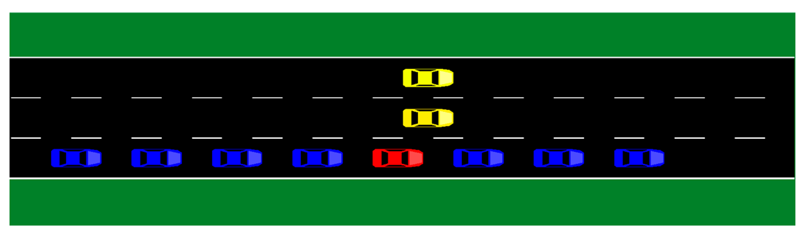
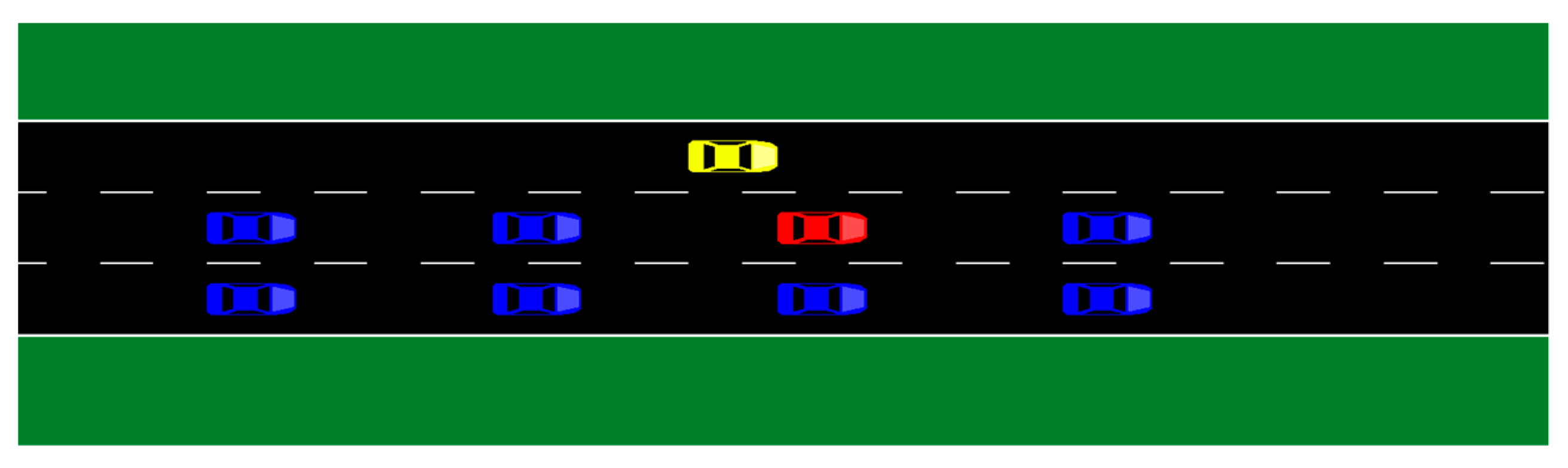
3.1. Simulation Experiment

SUMO, also known as Simulation of Urban MObility (version 1.14.0), is an open-source traffic simulation software used to simulate urban traffic flow, road networks, and traffic control systems [24]. In this section, we conduct simulation experiments using SUMO software (version 1.14.0) and analyze the results. In the simulation experiment, we set a test vehicle, seven virtual environmental vehicles, and several real environmental vehicles. The test vehicle is controlled by an autonomous vehicle planning and control algorithm, which remain to be tested. The seven virtual environmental vehicles are controlled by the methods proposed in this paper (Graph Theory and APF method), and the real environmental vehicles take actions according to the pre-determined actions.

To ensure that the simulation experiment is close to the real scene, the relevant constraints set in the experiment are as follows: the range of front wheel steering angle of the vehicle is 25 degrees to 25 degrees, the range of longitudinal acceleration of the vehicle is −0.4 g to 0.2 g, the rate of acceleration change is −2 g to 2 g, the maximum rate of front wheel steering angle change is 20 degrees per second, and the lateral acceleration is not more than 1 m/s². The experimental scenario is a one-way three-lane road with a lane width of 3.6 m and a vehicle width of 1.8 m. The following are the specific simulation scenarios, in which the red vehicle is the test vehicle, the blue vehicles are the virtual environmental vehicles, and the yellow vehicles are the real environmental vehicles. From bottom to top, they are lanes 1 to 3 respectively.

Scenario 1: The virtual environmental vehicles run around the test vehicle. At this time, a pair of slowly moving real environmental vehicles is on lanes 2 and 3 ahead. In this case, all virtual environmental vehicles need to change lanes and quickly pass through lane 1, as shown in Figure 6 and Figure 7.

Scenario 2: A real environmental vehicle moves slowly in lane 3, and virtual environmental vehicles form a two-column formation and pass through lanes 1 and 2, as shown in Figure 8

The final speed of the vehicle formation in this experiment reaching the expected speed value represents the completion of the entire lane changing and following control adjustment.

Figure 9 and Figure 10 show the results of vehicle trajectory planning in different scenarios using Graph Theory and Artificial Potential Fields.

Figure 9 shows the average speed of the target formation vehicles from an initial state of 0 in the scene. The vehicle starts from a standstill and the expected speed is set to 12 m/s. In the initial stage, due to different starting accelerations of the vehicles, the distance between adjacent vehicles in the longitudinal direction decreases as the speed gradually increases. The potential field force will generate a braking “command” for the following vehicles to ensure safe driving. Subsequently, based on Graph Theory and Artificial Potential Fields, road nodes are constructed to plan the optimal path to reach the target queue. Firstly, the lane-following state in each lane is maintained, and environmental vehicles on the second and third lanes are switched and merged into the first lane in 5 s and 11 s, respectively. This reduces the impact of the multiple merging of a single vehicle into the path on the overall state and improves safety and overall efficiency in this scenario.

Figure 10 shows the process of formation changes in Scenario 2. Scenario 2 is based on Scenario 1. When half of the vehicles in the fleet complete the lane change to the second lane, the longitudinal potential field between vehicles decreases for the other vehicles, and the overall fleet will experience an acceleration process. Then, when Graph Theory determines the parallel driving formation, it will cause significant speed fluctuations. The artificial potential field achieves fine-tuning of the vehicle’s position, and the total time for this process is 18 s.

Under the same conditions, if the RRT is used for vehicle trajectory generation, the implementation complexity is higher and the time consumption is longer. The specific parameter comparison is shown in the table below.

The above experiment combines Graph Theory and the Artificial Potential Field Method to generate the trajectory of virtual environment vehicles, which can achieve safe following and lane-changing scenarios of vehicles in complex environments, quickly control vehicle formation, and have small overall speed fluctuations.

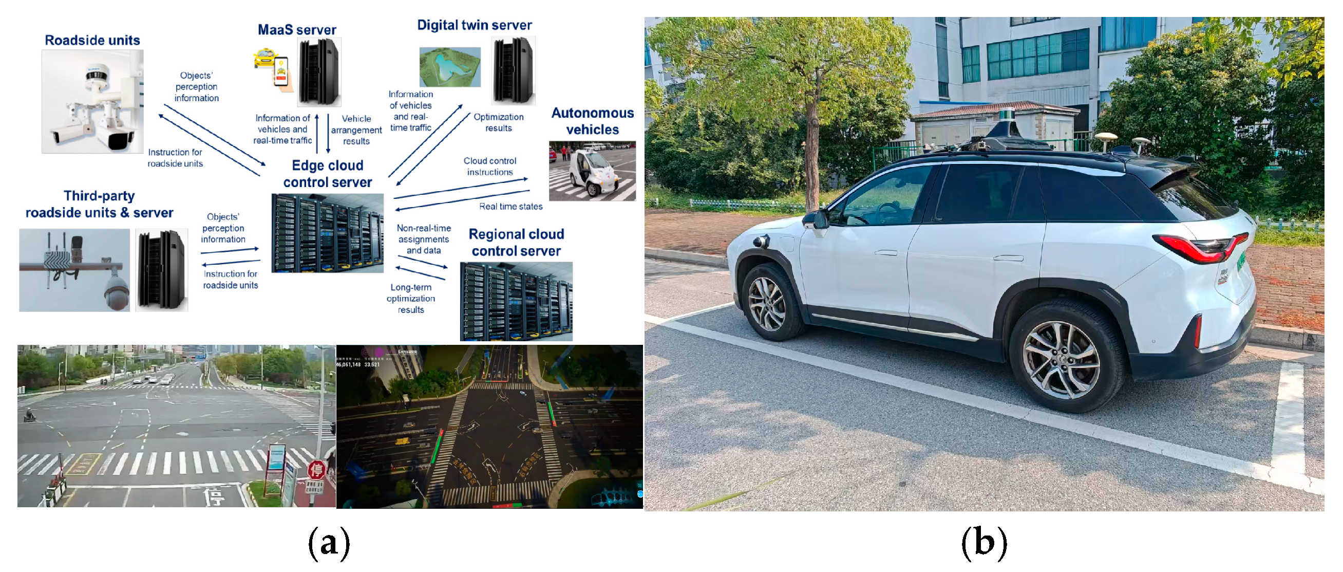
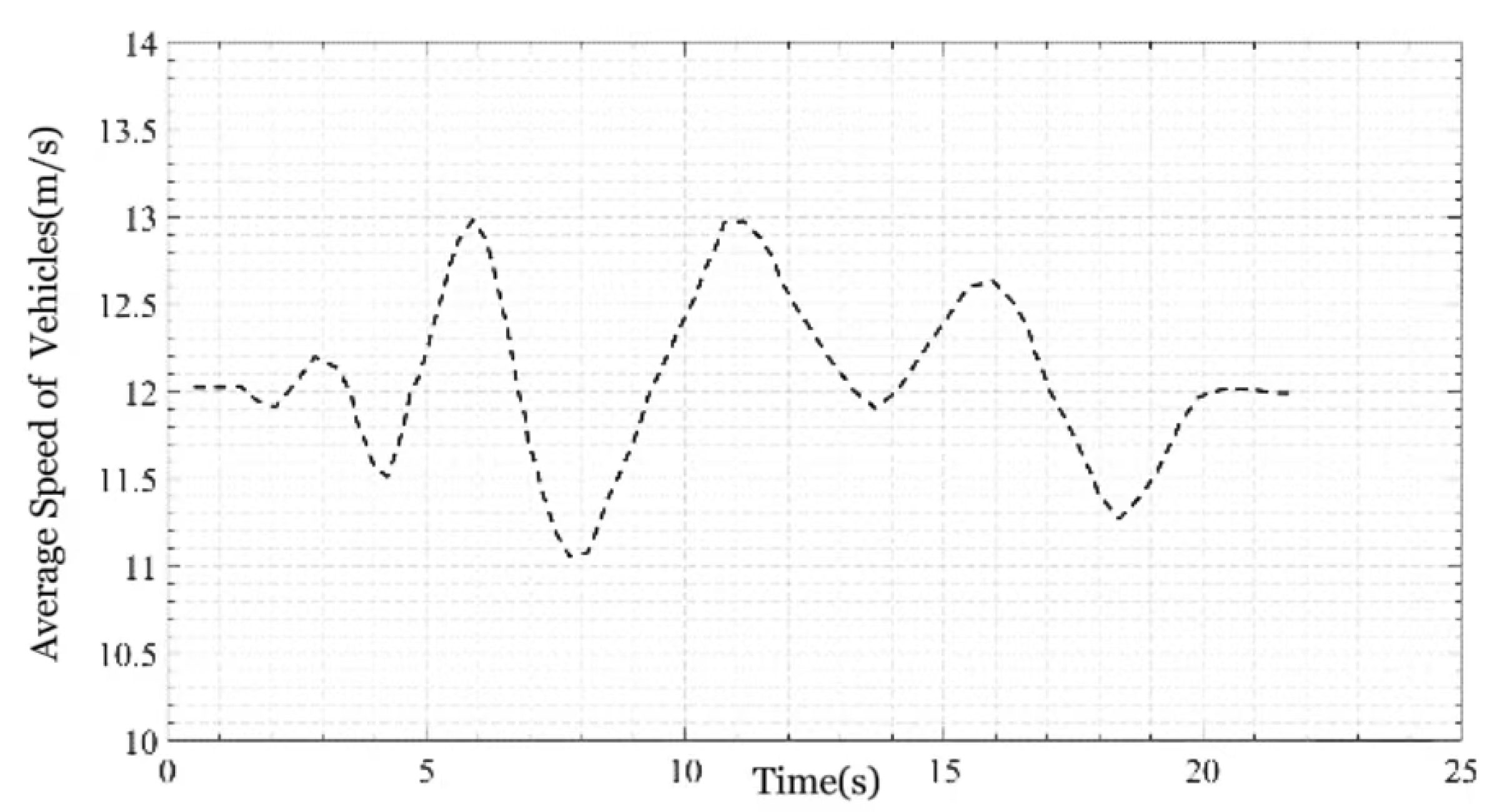
3.2. Field Experiment

We carried out real field experiments to validate the methods proposed in this study. The experiment was carried out on the Vehicle-Road-Cloud Integrated Platform in Suzhou High-Speed Railway New Town, where virtual-real fusion testing capabilities were developed by the Tsinghua University Suzhou Automotive Research Institute, as shown in the following Figure 11 and Figure 12.

Our lidar-camera fusion traffic environment perception method is divided into four steps: image feature extraction, point cloud feature extraction, BEV (Bird’s Eye View) feature fusion, and detection head of traffic environment information.

Image feature extraction: Since our framework needs to fuse image information from multiple surround-view cameras, we develop a fusion method based on the classical LSS (Lifting Stereo Segmentation) approach. LSS was initially designed for BEV semantic segmentation without including 3D target detection; therefore, we improved the fusion method by referring to the LSS architecture.

Point cloud feature extraction: In general, using a feature extraction network, our framework can use any point cloud converted to BEV features for the point cloud feature extraction module. One common approach is learning a parametric voxelization of the original points to reduce the Z-dimension and then using a network of sparse 3D convolutions to generate features in the BEV space efficiently. This paper uses PointPillars as our point cloud feature extraction module to implement point cloud feature extraction in the BEV space.

Fusion Module: To effectively fuse the BEV features from both the camera and LiDAR sensors, we propose a dynamic fusion module. Given two features under the same space dimension, an intuitive idea is to concatenate them and fuse them with learnable static weights. Inspired by the Squeeze-and-Excitation mechanism, we apply a simple channel attention module to select important fused features.

Detection head: In general, 3D object detection in autonomous driving is used to obtain the position, scale, orientation, and velocity of moving objects, such as pedestrians, vehicles, and obstacles. Without any modifications, we directly reuse the center-point detection head.

In the field experiment, road equipment and third-party devices collect road condition and vehicle position data with on-board sensors, which are processed and transmitted through edge cloud control servers and then uploaded to MaaS and digital twin servers. Autonomous vehicles utilize this information for real-time decision-making and path planning, while regional cloud control servers are responsible for long-term data storage and large-scale traffic management. Then we adapt the same scenarios as those in the simulation experiment. The experimental results are presented in Figure 13 and Figure 14.

Experimental results show that this method can quickly generate multiple vehicle trajectories in dynamic scenes, thereby improving the safety of autonomous vehicles. In Scenario 1, the test vehicle and surrounding vehicles recognize vehicles on lanes 2 and 3 on the path and quickly drive to lane 1 in a single queue. In Scenario 2, both lanes 1 and 2 are passable, and the vehicles in the convoy have regenerated their trajectories, achieving dual queue driving on lanes 1 and 2. In this experiment, we compared the method in the study with the RRT; our method in Scenario 1 took a total process of 23 s, while RRT took 45 s. The total process times for the two methods in Scenario 2 were 20 s and 39 s, respectively. The results show that our method outperforms RRT.

In contrast, the comparison of the data in

Table 1. Comparison with the RRT method in the simulation.

	Graph Theory and Artificial Potential Field Method	RRT
Scenario 1	21 s	36 s
Scenario 2	18 s	30 s

and

Table 2. Comparison with the RRT method in the field experiment.

	Graph Theory and Artificial Potential Field Method	RRT
Scenario 1	23 s	45 s
Scenario 2	20 s	39 s

reveals a noticeable difference in the time required to reach the final stable speed across the various methods. Specifically, the simulation experiments using Graph Theory and the Artificial Potential Field Method show a discrepancy of approximately 2 s when compared to the virtual-real fusion testing. In contrast, the RRT (Rapidly-exploring Random Tree) method exhibits a larger difference of about 9 s. These results suggest that the Graph Theory and Artificial Potential Field Method demonstrate superior performance and reliability when applied to real-world scenarios.

4. Conclusions

In this study, a testing scenario was established in a virtual environment based on real-world testing scenarios. By integrating Graph Theory and artificial potential field methods, vehicle trajectories were efficiently generated in response to dynamic changes in multiple environmental vehicles. Compared with traditional path planning research, the combination of real road scenes and virtual environments enhances the complexity and authenticity of scenarios, while the proposed methods improve adaptability to complex scenes and enable efficient path planning. However, this study primarily focused on overtaking and lane-changing scenarios, which limits its application to more diverse and extreme traffic conditions. Future research should narrow its scope to specific challenges, such as high-density urban intersections or adverse weather conditions, where vehicle interactions and uncertainties are more pronounced. Additionally, the simplified vehicle dynamics model and the limited scale of real-world testing present constraints that need to be addressed to validate the approach in larger-scale and more realistic environments.

It is also worth noting that our current work focuses on proposing a new virtual reality fusion testing method for trajectory generation and testing of autonomous vehicles in complex traffic environments. Although our approach differs from the system theory-based process analysis (STPA) framework and test scenario development method proposed by Khastgir et al. [10] in terms of research methods and application scenarios, we recognize the potential synergies between the different methods. In future work, we plan to explore how to combine our proposed method with other existing frameworks, such as the STPA-based approach, to achieve more comprehensive and robust testing of autonomous driving systems. This integration could help address some of the limitations identified in this study and further enhance the safety and reliability of the testing of autonomous vehicles.

References

1. Xu, L.; He, B.; Zhou, H.; He, J. Impact and Revolution on Law on Road Traffic Safety by Autonomous Driving Technology in China. Comput. Law Secur. Rev. 2023, 51, 105906. [Google Scholar] [CrossRef]
2. Zheng, Y.; Wang, J.; Li, X.; Yu, C.; Kodaka, K.; Li, K. Driving risk assessment using cluster analysis based on naturalistic driving data. In Proceedings of the 17th International IEEE Conference on Intelligent Transportation Systems (ITSC), Qingdao, China, 8–11 October 2014; pp. 2584–2589. [Google Scholar]
3. Ning, H.; Xu, W.; Zhou, Y.; Gong, Y.; Huang, T.S. A general framework to detect unsafe system states from multisensor data stream. IEEE Trans. Intell. Transp. Syst. 2009, 11, 4–15. [Google Scholar] [CrossRef]
4. Xiong, X.X.; Chen, L.; Liang, J.; Cai, Y.F.; Jiang, H.B. Simulation study of driving risk discrimination method based on driver collision avoidance behavior. Automot. Eng. 2019, 41, 153–160. [Google Scholar]
5. Arbabzadeh, N.; Jafari, M. A data-driven approach for driving safety risk prediction using driver behavior and roadway information data. IEEE Trans. Intell. Transp. Syst. 2017, 19, 446–460. [Google Scholar] [CrossRef]
6. Xu, S.; Zhu, J. Estimating Risk Levels of Driving Scenarios through Analysis of Driving Styles for Autonomous Vehicles. arXiv 2019, arXiv:1904.10176. [Google Scholar] [CrossRef]
7. SAE On-Road Automated Vehicle Standards Committee. Taxonomy and definitions for terms related to on-road motor vehicle automated driving systems. SAE Standard J. 2014, 3016, 1. [Google Scholar]
8. Klischat, M.; Althoff, M. Generating Critical Test Scenarios for Automated Vehicles with Evolutionary Algorithms. In Proceedings of the 2019 IEEE Intelligent Vehicles Symposium (IV), Paris, France, 9–12 June 2019; pp. 2352–2358. [Google Scholar]
9. Nalic, D.; Mihalj, T.; Bäumler, M.; Lehmann, M.; Eichberger, A.; Bernsteiner, S. Scenario Based Testing of Automated Driving Systems: A Literature Survey. FISITA Web Congr. 2020, 2020, 1. [Google Scholar]
10. Riedmaier, S.; Ponn, T.; Ludwig, D.; Schick, B.; Diermeyer, F. Survey on Scenario-Based Safety Assessment of Automated Vehicles. IEEE Access 2020, 8, 87456–87477. [Google Scholar] [CrossRef]
11. Review of Scenario-based Virtual Validation Methods for Automated Vehicles. China J. Highw. Transp. 2019, 32, 1–19. [CrossRef]
12. Drechsler, M.F.; Peintner, J.; Reway, F.; Seifert, G.; Riener, A.; Huber, W. MiRE, A Mixed Reality Environment for Testing of Automated Driving Functions. IEEE Trans. Veh. Technol. 2022, 71, 3443–3456. [Google Scholar] [CrossRef]
13. Riedmaier, S.; Schneider, D.; Watzenig, D.; Diermeyer, F.; Schick, B. Model Validation and Scenario Selection for Virtual-Based Homologation of Automated Vehicles. Appl. Sci. 2021, 11, 35. [Google Scholar] [CrossRef]
14. Dahmen, U.; Osterloh, T.; Roßmann, J. Structured Validation of AI-Based Systems by Virtual Testing in Simulated Test Scenarios. Appl. Intell. 2023, 53, 18910–18924. [Google Scholar] [CrossRef]
15. Campos, C.; Leitão, J.M.; Pereira, J.P.; Ribas, A.; Coelho, A.F. Procedural Generation of Topologic Road Networks for Driving Simulation. In Proceedings of the 2015 10th Iberian Conference on Information Systems and Technologies (CISTI), Aveiro, Portugal, 17–20 June 2015; pp. 1–6. [Google Scholar]
16. Meyer, M. Graph-Based Generation of OpenSCENARIO-Driving-Scenarios for Virtual Validation of Automated Driving Functions. PhD Thesis, Technische Hochschule Ingolstadt, Ingolstadt, Germany, 2022. [Google Scholar]
17. Thieling, J.; Mathar, M.; Roßmann, J. Automated Generation of Virtual Road Scenarios For Efficient Tests of Driver Assistance Systems. In Proceedings of the 2017 IEEE AUTOTESTCON, Schaumburg, IL, USA, 9–15 September 2017; pp. 1–9. [Google Scholar]
18. Wang, P.; Gao, S.; Li, L.; Sun, B.; Cheng, S. Obstacle Avoidance Path Planning Design for Autonomous Driving Vehicles Based on an Improved Artificial Potential Field Algorithm. Energies 2019, 12, 2342. [Google Scholar] [CrossRef]
19. Mora, M.C.; Tornero, J. Path Planning and Trajectory Generation Using Multi-Rate Predictive Artificial Potential Fields. In Proceedings of the 2008 IEEE/RSJ International Conference on Intelligent Robots and Systems, Nice, France, 22–26 September 2008; pp. 2990–2995. [Google Scholar]
20. Xie, S.; Hu, J.; Bhowmick, P.; Ding, Z.; Arvin, F. Distributed Motion Planning for Safe Autonomous Vehicle Overtaking via Artificial Potential Field. IEEE Trans. Intell. Transp. Syst. 2022, 23, 21531–21547. [Google Scholar] [CrossRef]
21. Khatib, O. Real-Time Obstacle Avoidance for Manipulators and Mobile Robots. Int. J. Robot. Res. 1986, 5, 90–98. [Google Scholar] [CrossRef]
22. Chiang, H.-T.; Malone, N.; Lesser, K.; Oishi, M.; Tapia, L. Path-Guided Artificial Potential Fields with Stochastic Reachable Sets for Motion Planning in Highly Dynamic Environments. In Proceedings of the 2015 IEEE International Conference on Robotics and Automation (ICRA), Seattle, WA, USA, 26–30 May 2015; pp. 2347–2354. [Google Scholar]
23. Das, M.S.; Sanyal, S.; Mandal, S. Navigation of Multiple Robots in Formative Manner in an Unknown Environment Using Artificial Potential Field Based Path Planning Algorithm. Ain Shams Eng. J. 2022, 13, 101675. [Google Scholar] [CrossRef]
24. Krajzewicz, D.; Erdmann, J.; Behrisch, M.; Bieker, L. Recent development and applications of SUMO-Simulation of Urban MObility. Int. J. Adv. Syst. Meas. 2012, 5. [Google Scholar] [CrossRef]
Figure 1. Schematic of the road coordinate system.
Electronics 14 01000 g001
Figure 2. Schematic diagram of the lane line potential field.
Electronics 14 01000 g002
Figure 3. Lane potential field for lane changing to the right.
Electronics 14 01000 g003
Figure 4. Design of environmental vehicle potential field range.
Electronics 14 01000 g004
Figure 5. Changes in the environmental vehicle potential field.
Electronics 14 01000 g005
Figure 6. Initial state.
Electronics 14 01000 g006
Figure 7. Schematic representation of Scenario 1.
Electronics 14 01000 g007
Figure 8. Schematic representation of Scenario 2.
Electronics 14 01000 g008
Figure 9. Vehicle formation average speed change in Scenario 1.
Electronics 14 01000 g009
Figure 10. Vehicle formation average speed change in Scenario 2.
Electronics 14 01000 g010
Figure 11. The virtual-real fusion testing platform: (a) testing platform; (b) testing vehicle.
Electronics 14 01000 g011
Figure 12. BEV perception results.
Electronics 14 01000 g012
Figure 13. The virtual-real fusion testing of Scenario 1.
Electronics 14 01000 g013
Figure 14. The virtual-real fusion testing of Scenario 2.
Electronics 14 01000 g014