Abstract
Colorectal cancer (CRC) has a relatively high five-year survival rate compared to other cancers; however, this rate drops significantly in patients with malignant CRC. One critical factor in palliative care decision-making is the ability to accurately predict patient survival, with the six-month survival period commonly used as a threshold. In this study, we evaluated the performance of five machine learning models—logistic regression, decision tree, random forest, multilayer perceptron, and extreme gradient boosting (XGBoost)—in predicting six-month survival for patients with malignant CRC using a publicly available synthetic dataset containing 11,774 samples and 51 features. The models were trained and validated using five-fold cross-validation, and the synthetic minority oversampling technique (SMOTE) was applied to address class imbalance. Among the models, XGBoost demonstrated the highest performance, achieving 95% accuracy, precision, recall, and F1-score, along with 90% specificity. Feature importance analysis identified smoking status and surgical history as key factors influencing model predictions. These findings highlight the potential of tree-based machine learning models in supporting timely and informed palliative care decisions, while also providing insights into handling data imbalance and optimizing model parameters in survival prediction tasks.
1. Introduction
Colorectal cancer (CRC) is the third leading cause of cancer-related deaths both in Korea and globally [1]. From 1999 to 2020, the incidence rate of CRC in Korea increased significantly, with a standardized age-adjusted rate of 7.2 per 100,000, making it the second most common cancer after stomach cancer [2]. The five-year survival rate of CRC in Korea is 75.6%, surpassing the 65% rate in the United States and ranking highest worldwide [3]. Specifically, early detection and treatment significantly improve survival outcomes. For instance, the five-year survival rate for localized CRC (limited to the colon) can reach approximately 90% [4]. However, if the cancer metastasizes to the lymph nodes or other organs, the survival rate drops sharply, with an approximately 14% five-year survival rate for metastatic CRC [5]. Therefore, early detection remains critical for long-term survival in CRC, and many studies have focused on survival-period prediction, as it aids in optimizing treatment strategies and improving patient prognosis [5,6,7]. Accurate predictions are essential for informed treatment decisions and enhancing survival outcomes.
Although predicting the five-year survival rate and early detection are crucial, an often-overlooked but equally important aspect is deciding the treatment after diagnosis. Specifically, patients and doctors must decide whether to pursue aggressive treatments, such as surgery and chemotherapy, with the hope of eliminating the tumor, or palliative or supportive care to enhance the patient’s quality of life when the cancer has significantly progressed. This empowers patients with autonomy over their treatment decisions and lives. Opting for palliative care allows the patient and their family to promptly prepare for the future course of action, such as hospice or long-term care. Although CRC has a high five-year survival rate, it progresses to metastatic CRC (mCRC) in 40–60% of patients, and 80% of them are incurable [8,9,10,11]. In clinical practice and previous studies, a minimum of six months has been typically employed as the threshold for palliative care [12,13,14], and patients who receive appropriate palliative care exhibit extended survival, reduced treatment costs, decreased healthcare-resource utilization, and improved quality of life [15,16,17].
Survival-period prediction of patients with CRC based on a six-month threshold for palliative-care decisions is influenced by various clinical factors and lifestyle choices, leading to challenges owing to data imbalance. Traditional statistical methods face limitations in adequately reflecting the multivariate factors and nonlinear relationships involved in predicting the survival periods for CRC patients [16,17,18]. By contrast, machine learning techniques offer the advantage of processing large-scale data and capturing nonlinear patterns, leading to their widespread application in survival-prediction tasks [19,20,21,22]. Ensemble models, such as extreme gradient boosting (XGBoost), and neural networks have demonstrated superior performance among various survival-prediction models [23,24,25], and oversampling techniques have been employed to address data-imbalance issues [26,27,28]. A recent study on CRC survival prediction trained various models, including naïve Bayes, random forest (RF), and XGBoost models, on the data of 31,916 patients with colorectal adenocarcinoma [29]. The findings demonstrated that XGBoost exhibited the highest performance, achieving a 77% accuracy for predicting cancer-specific survival. Furthermore, it emphasized that cancer staging is the most influential factor for survival outcomes. However, there are inherent limitations in predicting CRC outcomes using machine learning. Specifically, owing to the statistical characteristics of CRC survival rates, which are relatively high compared to those of other cancers, the collected data are inherently imbalanced, which increases the risk of overfitting as model complexity increases. Additionally, survival-period-prediction models vary according to the disease characteristics, dataset composition, and target variables [30,31,32,33]. Therefore, previous studies have investigated the performance and hyperparameter metrics of various machine learning models, ranging from shallow [34,35] to deep neural networks [36,37] and ensemble models [38,39].
In the absence of a standardized data format and comprehensive datasets at the national level [40], developing a robust model is challenging owing to the variability in the data-collection methods and medical terminology employed across different hospitals and institutions. Therefore, in this study, the primary goal was to evaluate models that are robust to class imbalance within a comprehensive medical dataset. After identifying the most robust model, the oversampling technique was applied to further assess whether it could enhance the model’s performance. We hypothesized that (1) models that are robust to class imbalance will demonstrate superior predictive performance on a comprehensive medical dataset, (2) applying an oversampling technique will further enhance the performance of the most robust model, and (3) identifying key predictive features will provide essential insights for developing personalized patient management strategies.
2. Materials and Methods
2.1. Dataset Description
The synthetic dataset, consisting of 15,000 samples and 52 features, as detailed in Table 1, was generated by the National Cancer Center using a generative adversarial network (GAN) based on their own data from 1263 colorectal cancer patients. The features used in this study include a range of patient demographic, pathological, staging and metastasis, and genetic mutation data. As shown in Table 1, patient demographic information includes age (feature 1), height (feature 41), weight (feature 42), type of drink (feature 39), smoking status (feature 40), operation status (feature 49), and chemotherapy status (feature 50). Pathological characteristics are represented by features 2 to 8, including mucinous tumors (feature 2), signet ring cell tumors (feature 3), adenocarcinoma (feature 4), carcinoid tumors (feature 5), neuroendocrine carcinoma (feature 6), squamous cell carcinoma (feature 7), and malignant neoplasm (feature 8). Staging and metastasis data include features 9–23 (tumor size and invasion degree, T1–T4), features 24–33 (lymph node metastasis degree, N1–N3), and features 34–37 (distant metastasis, M1). Finally, genetic mutations and biomarkers are represented by feature 43 (EGFR), feature 44 (MSI), feature 45 (KRAS mutation Exon 2), feature 46 (KRAS mutation), feature 47 (NRAS mutation), and feature 48 (BRAF mutation). This dataset, created and publicly released by the National Cancer Center, was derived from their proprietary patient data. The variable characteristics and correlations within the actual and synthetic datasets are shown in Figure 1. We excluded data from samples of patients who are currently alive and have a survival period of less than six months, as they may potentially survive beyond this period, within the 15,000 samples. Accordingly, in this study, we used 11,774 samples for model training and performance testing. The analysis involved 51 features and one binarized target variable, with no missing values for any feature. Also, to identify the statistical differences between classes, we conducted independent t-tests for continuous variables such as age, height, and weight, and applied chi-square tests to evaluate the differences in frequency distributions of categorical variables across classes. A significance level of 0.05 was applied to all tests.

Table 1.
Characteristics of the synthetic public dataset of patients with CRC, provided by the National Cancer Center.
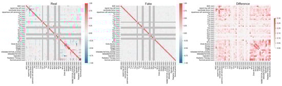
Figure 1.
Variable characteristics and correlations within the actual and synthetic datasets provided by the National Cancer Center. The left panel (Real) represents the correlation structure of the original dataset, while the middle panel (Fake) shows the correlation matrix of the synthetic dataset. The right panel (Difference) highlights the absolute differences between the real and synthetic correlation structures, with darker-red regions indicating greater discrepancies.
2.2. Data Preprocessing
The dataset comprising clinical information, lifestyle factors, and treatment-related features from deceased CRC patients was randomly divided into training and test sets in an 80:20 ratio, while also accounting for the class imbalance during the division, and subsequently subjected to five-fold cross-validation, as shown in Figure 2. To ensure the robustness of the validation process, the validation set was constructed by maintaining the same class distribution as the training set to address potential concerns regarding distribution imbalances. In all datasets, patients with a survival period of ≤180 days were classified into the defined Class 0 and those with a survival period of >180 days were classified into Class 1 based on the six-month threshold for guiding palliative-care decisions. The survival period was calculated based on the diagnosis date of cancer. Furthermore, to address the imbalance issue between the classes, the synthetic minority oversampling technique (SMOTE) was adopted exclusively for the highest-performance model. This approach aimed to balance the dataset and subsequently evaluate whether the predictive performance improved after further analysis. All analyses were conducted in Python (version 3.12.4) using Google Colab’s GPU environment with a Tesla T4 GPU.
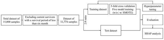
Figure 2.
Schematic overview of the six-month survival prediction in patients with malignant colorectal cancer. SMOTE: synthetic minority oversampling technique; SHAP: Shapley additive explanations.
2.3. Construction of Predictive Models
In this study, the performances of five predictive models were compared, and the best hyperparameter search was implemented using the grid-search function. Prior to the application of SMOTE, each model was configured with an option to automatically adjust the weights of each class, thereby enhancing the importance assigned to classes with lower representation in the model. The equations and reasons for selecting each algorithm are detailed in the following. In all models, the prediction target was defined as Y = 0 for survival durations of 180 days or less and Y = 1 for durations exceeding 180 days:
- (1)
- The logistic regression (LR) model [41] is commonly employed for binary classification tasks, due to its ability to express the relationship between input features and the target variable in a linear fashion. The model is mathematically expressed as follows:where P(Y) is the probability of the dependent variable, is the intercept, and represents the regression coefficient for each predictor, . Logistic regression assumes that the log-odds of the dependent variable are linearly related to the independent variables. This makes it particularly suitable for datasets where the relationship between the predictors and the target variable is approximately linear. This model served as a baseline for comparing the performance of the other models.
- (2)
- The decision tree (DT) model [42] is a nonparametric algorithm widely used for classification tasks due to its ability to split data into homogeneous subsets based on specific criteria. The model is built upon a recursive partitioning process, where each split aims to maximize the purity of the resulting subsets. One commonly used criterion for assessing split quality is the Gini index, calculated as follows:where is the metric for assessing the purity of splits and represents the probability of the data point belonging to class . Lower Gini values indicate greater homogeneity within the subsets. Decision trees are particularly valued for their transparency and ease of interpretability, as the decision-making process can be visualized as a tree-like structure.
- (3)
- The random forest (RF) model [43] is an ensemble learning algorithm that combines multiple decision trees to improve classification accuracy and mitigate overfitting. The model aggregates predictions from individual trees through majority voting, as expressed in the following:where is the final prediction, represents the prediction made by the -th tree, and the overall classification result is determined by the mode of these predictions. This approach enables random forest to capture complex, nonlinear relationships within the data while maintaining robustness against noise.
- (4)
- The multilayer perceptron (MLP) model [44] is a type of feedforward neural network designed to capture complex, nonlinear relationships within data by leveraging multiple hidden layers. The output of a neuron in this model is given by the following:where is the activation function (ReLU in the hidden layers), represents the weights associated with each input feature , is the bias, and is the number of input features. For binary classification, the output layer employs a sigmoid activation function, transforming the output into a probability value between 0 and 1. This value is interpreted as Y = 1 if P() > 0.5 and Y = 0 otherwise, ensuring compatibility with classification tasks. The MLPClassifier function was used with the following hyperparameters: activation: set to ‘relu’, enabling the model to capture nonlinear relationships efficiently by introducing nonlinearity in each layer.
- (5)
- The XGBoost (extreme gradient boosting) model [45] is a gradient-boosting-based ensemble learning technique that is renowned for its high predictive performance and computational efficiency, particularly when working with high-dimensional datasets. Its objective function is defined as follows:where represents the model’s learnable parameters, L is the loss function that measures the error between the true value, , and the predicted value, , and () is the regularization term that penalizes overly complex models to prevent overfitting. For binary classification, XGBoost calculates the probability, P(Y), by aggregating the outputs of multiple decision trees. These outputs, expressed as logits, are transformed into probabilities using the sigmoid function. The final class label is determined by applying a threshold: P(Y) > 0.5 corresponds to Y = 1, while P(Y) ≤ 0.5 corresponds to Y = 0.
2.4. Oversampling Method
SMOTE [46], defined in Equation (6), is applied to address the data imbalance resulting from differences in the survival period, where one class (i.e., survival period ≤ 6 months) may have significantly fewer instances than the other. The synthetic samples are generated by interpolation between a selected minority class sample, , and one of its k-nearest neighbors, .
where xnew represents the synthetic sample generated via interpolation between the selected minority class sample, xi, and one of its k-nearest neighbors, . λ is a multiplicative value sampled from a uniform distribution between 0 and 1, ensuring that synthetic samples are evenly distributed along the line segment between the original sample and its neighbor, rather than clustering near the original sample. In this study, the dataset exhibited the following class imbalance, and synthetic samples were generated to balance the dataset more evenly. Specifically, with 1047 samples for class 0 and 10,727 samples for class 1, synthetic samples were generated solely for the minority class (class 0) to address the imbalance and ensure a more uniform distribution. Regarding the choice of k, the default value of k = 5 was used in the SMOTE implementation. We used the imblearn library version 0.12.4 to apply the SMOTE technique in this study.
2.5. Performance Metrics
The performances of the models were evaluated using accuracy, precision, recall, F1-score, and specificity metrics based on their true-positive (TP), false-positive (FP), true-negative (TN), and false-negative (FN) values, which were computed. F1-score is defined as the weighted harmonic mean of precision and recall, thereby representing the overall model performance. In this study, the criteria for selecting the best model were based on balanced performance, which refers to a model’s ability to perform consistently well across multiple metrics without prioritizing one at the expense of the others.
2.6. Exploring Feature Contributions via Shapley Additive Explanations (SHAP)
This study employed SHAP, a technique for interpreting the classification output of the best predictive model and clarifying the relationship between features and the six-month survival rate of patients with CRC. We employed Tree SHAP, which is optimized for tree-based models such as gradient-boosting algorithms [47]. Tree SHAP offers computational efficiency and precise feature attribution by leveraging the structural properties of decision trees, making it suitable for interpreting the predictive relationships between features and outcomes in this context.
The adoption of Tree SHAP in this study was guided by its compatibility with the tree-based architecture of the machine learning framework employed, facilitating the extraction of meaningful insights into feature contributions related to the six-month survival rate of CRC patients. This methodology ensured that the interpretation process remained aligned with the model structure and data characteristics.
3. Results
3.1. Model Performance
As stated previously, we compared the performances of five machine learning models: LR, DT, RF, MLP, and XGBoost. The hyperparameters applied to each model through a grid search are summarized in Table 2. The results of the cross-validation performance metrics for each model using the training dataset are listed in Table 3. The results on the test dataset are listed in Table 4. XGBoost demonstrated the highest robustness, achieving the best performance in accuracy (0.82), precision (0.84), recall (0.82), and F1-score (0.83), underscoring its superior performance among the evaluated models. Despite the implementation of weighting adjustments to address the data-imbalance issue across all models, the specificity remained significantly low, ranging from 0.12 to 0.54. Therefore, we retrained the XGBoost model after applying oversampling through SMOTE, which significantly enhanced specificity to 90%, as well as other metrics (0.95), as indicated by the confusion matrix shown in Figure 3.
Table 2.
Hyperparameters used in the models.
Table 3.
Cross-validation performance metrics for the five models using the training dataset.
Table 4.
CRC classification performances of the five models on the test dataset.
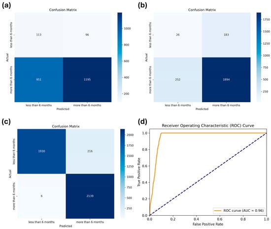
Figure 3.
Confusion matrices of (a) logistic regression, (b) extreme gradient boosting (XGBoost) before applying the synthetic minority oversampling technique (SMOTE), and (c) XGBoost after applying SMOTE for the test dataset. (d) Receiver Operating Characteristic (ROC) curve for the XGBoost after applying SMOTE, showing the trade-off between sensitivity and specificity across different thresholds.
3.2. Feature Contributions via SHAP
By utilizing the Tree SHAP function, specifically designed for boosting models, the features influencing the expected survival period of patients with colorectal cancer (CRC) and the importance of features in the SMOTE-applied XGBoost model were interpreted. Among the 51 features, the top 20 were identified based on their SHAP values, as shown in Figure 4. The most prominent features influencing the model results were smoking and operation, as demonstrated in Figure 4a, which summarizes the average SHAP values to highlight the overall importance of each variable. Smoking status, specifically whether the patient was a current smoker, had the greatest influence on the model’s predictions, followed by a history of cancer surgery.
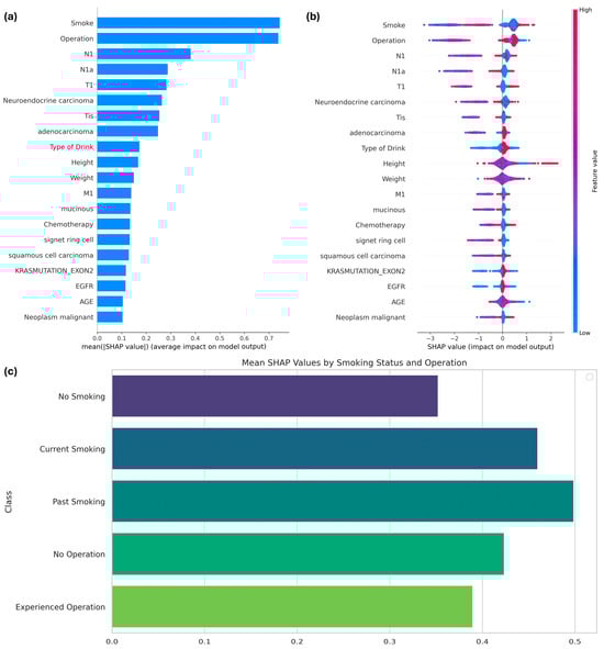
Figure 4.
(a) SHAP values of features influencing the performance of the XGBoost model with SMOTE; (b) SHAP summary plot; and (c) mean SHAP values by class for the two primary features.
Figure 4b provides a detailed visualization of how each feature impacts predictions at the individual level. For smoking, lower feature values (e.g., non-smokers) were associated with higher SHAP values, indicating an increased likelihood of survival beyond six months. Conversely, higher feature values for smoking (e.g., current smokers) correlated with negative SHAP values, reflecting a reduced survival probability. Similarly, for the operation feature, individuals with a value of 1 (indicating prior surgery) exhibited consistently higher SHAP values, suggesting that surgical intervention positively influences survival outcomes.
Figure 4c delves deeper into subgroup-specific analyses for smoking and operation. Categorical variables for smoking were defined as follows: 0 indicated no smoking history, 1 indicated current smoking, and 2 indicated a history of smoking. Non-smokers demonstrated the highest mean SHAP values, highlighting a stronger association with prolonged survival compared to both current and past smokers. For the operation feature, patients with a history of surgery showed consistently higher SHAP values than those without surgical intervention, further emphasizing its positive role in survival.
The subgroup-specific analyses for smoking and operation variables were conducted as follows: SHAP values for each category within the respective variables were separately calculated and visualized. For the smoking variable, SHAP values were grouped into three categories—0 (no smoking), 1 (current smoking), and 2 (history of smoking)—based on their corresponding indices in the validation dataset. Similarly, for the operation variable, SHAP values were categorized into two groups—0 (no operation history) and 1 (operation history). The mean SHAP values for each subgroup were computed to assess the average contribution of these categories to the model’s predictions. These values were then visualized using bar plots to highlight the relative impacts of each subgroup on the target variable.
The three subplots in Figure 4 are intrinsically linked. Figure 4a provides a global ranking of variable importance, while Figure 4b explores the variability in feature contributions at the individual level. Building on this, Figure 4c focuses on subgroup-specific SHAP values, illustrating how categorical distinctions such as smoking status and surgical history interact with survival predictions. Together, these visualizations provide a comprehensive understanding of both the global and localized impact of key features.
This analysis underscores the critical role of smoking history and surgical intervention in predicting survival outcomes. Non-smokers exhibit a higher likelihood of surviving beyond six months, whereas current smokers face increased risks. Additionally, a history of surgical intervention positively correlates with prolonged survival, making it a significant prognostic factor. These findings offer valuable insights for tailoring clinical strategies to improve outcomes for CRC patients.
4. Discussion
4.1. Insights and Future Studies
Predicting the six-month survival period of patients with CRC is crucial for guiding timely palliative-care decisions and optimizing treatment strategies. In this study, we employed five machine learning models to predict the six-month survival rate of patients with malignant CRC, with the aim of supporting informed treatment decisions. Despite the limitation that CRC generally has a high survival rate, which leads to a significantly smaller dataset for training machine learning models on data of patients with shorter survival periods, the issue of significantly low specificity caused by data imbalance was effectively addressed using SMOTE, and the superior predictive performance of XGBoost was confirmed. Additionally, we identified key features that influence the prediction of the six-month survival period, such as smoking status and surgical history, as well as the contributions of various other classes. Among the stages of mCRC, the initial stage of lymph node involvement (N1) was identified as the most significant factor influencing the six-month survival rate. N1 is a criterion for Stage III CRC and can significantly decrease the five-year survival rate (ranging from 22 to 69%) of patients with CRC. Adenocarcinoma was identified as the most significant feature among cancer types for predicting six-month survival.
XGBoost, a well-established tree ensemble method that seamlessly combines bagging and boosting techniques, is renowned for its consistently exceptional predictive performance across various medical domains [48,49,50]. Additionally, our results are comparable to the recent findings of a study on annual survival prediction for patients with CRC which included patients with predicted survival periods from one to five years [29]. The authors also reported the excellent accuracy of ensemble tree models, such as RF and XGBoost, on the test datasets; however, they achieved low sensitivity and specificity. Nevertheless, our results demonstrated that both sensitivity and specificity improved after applying SMOTE. Additionally, we confirmed that smoking status has a significant impact on feature importance, while history of surgery was aligned with the findings of previous studies [25,29,50]. A previous study has consistently shown that smoking negatively affects the prognosis of colorectal cancer (CRC) patients. In particular, a meta-analysis indicated that both current and former smoking were associated with poorer survival outcomes after CRC diagnosis. Specifically, current smokers showed an increased 30-day mortality rate of 49% to 100% compared to never smokers, and the overall all-cause mortality was 1.26 times higher for current smokers. These findings strongly support the detrimental effects of smoking on survival after CRC diagnosis [51]. Unlike the aforementioned study, which explored long-term survival prediction, the present study incorporated features such as smoking and alcohol consumption status to assess their impact on short-term prognosis. For example, a recent study suggested a novel approach based on machine learning models to predict one-, three-, and five-year survival, as well as overall and cancer-specific mortality, achieving approximately 80% accuracy across all tasks [52]. This study effectively demonstrated the applicability of AI-driven models in colorectal cancer prognosis by leveraging advanced hyperparameter optimization techniques.
In contrast, the present study focused on predicting six-month survival, a clinically significant threshold for palliative-care decisions. By narrowing the prediction window to a more immediate timeframe, the model achieved higher predictive performance, with the XGBoost classifier attaining 95% accuracy, precision, recall, and F1-score, along with 90% specificity. These findings highlight the potential of tree-based machine learning models in supporting timely clinical decision-making, particularly for patients with malignant CRC requiring urgent treatment planning.
However, it is difficult to generalize that only tree models are superior based on our study results, as other recent studies on annual survival prediction in patients have shown that LR outperforms tree-based and boosting models [53]. Such differences arise owing to the composition and characteristics of the datasets used; therefore, future studies must compare various machine learning models to identify prediction models that are suitable for specific dataset compositions.
Additionally, the performance of the models prior to the application of SMOTE indicated that although LR assumes linearity in its learning process, resulting in diminished learning capability with nonlinear data, it is less prone to overfitting than tree-based and neural-network models under data imbalance. Conversely, although tree-based and neural-network models demonstrate superior learning performance, they are vulnerable to overfitting under data imbalance. Recent reports have highlighted the superior performance of mixed models that leverage the advantages of diverse algorithms [54,55]. Therefore, future studies should focus on addressing the data-imbalance issue using sampling techniques and explore better solutions through advanced modeling.
4.2. Limitations
This study has several limitations that should be acknowledged. While the synthetic dataset reflects the statistical patterns of the original data, it inherently carries limitations, particularly in terms of generalizability. As shown in Figure 1, synthetic data may not fully capture the complex variability inherent in real clinical data, and their accuracy is dependent on the training data and the performance of the GAN model. Therefore, uncertainties may arise regarding the exact replication of clinical realities, which could impact the robustness of the model’s predictions when applied to real-world cases. Also, although SMOTE was applied exclusively to XGBoost based on its overall superior performance metrics, the findings cannot be generalized to the performance of other models.
Despite these limitations, this study demonstrates the feasibility of developing a predictive model based on the 180-day threshold, which serves as a criterion for distinguishing between palliative and aggressive treatment. Even though the synthetic data generation process may weaken the correlations between variables compared to real data, complicating feature extraction, effective models are still capable of identifying important variables influencing survival duration. This suggests the potential for future validation with high-quality, balanced real clinical data to provide clearer and more definitive results.
Therefore, this study not only highlights the potential of using synthetic data for predictive modeling in the context of data access challenges in the medical field but also demonstrates the possibility of constructing relatively robust models, even in the face of data scarcity and limitations. The findings offer valuable insights for future research directions, especially in relation to the application of the 180-day threshold for treatment decision-making.
5. Conclusion
This study demonstrated that XGBoost can effectively predict the six-month survival of patients with mCRC and that SMOTE successfully addresses the data-imbalance issue. Additionally, we identified the key features influencing the predictions of the models, thereby facilitating informed decisions regarding treatment options and expected quality of life. However, further research is required to evaluate the models on actual clinical datasets and enhance modeling approaches to better handle data-imbalance issues, especially given the limited studies focusing specifically on short-term survival predictions like the six-month threshold, which remains underexplored despite its critical importance for timely palliative care and treatment optimization.
Author Contributions
Conceptualization, J.L. and E.K.; methodology, E.K.; software, J.L. and Y.K.; validation, Y.K. and E.K.; formal analysis, Y.C.; investigation, J.L. and Y.K.; resources, J.L.; data curation, E.K.; writing—original draft preparation, J.L. and Y.C.; writing—review and editing, Y.K. and E.K.; visualization, J.L. and Y.C.; supervision, E.K.; project administration, E.K.; funding acquisition, J.L. All authors have read and agreed to the published version of the manuscript.
Funding
This research was supported by the Basic Science Research Program through the National Research Foundation of Korea (NRF) funded by the Ministry of Education (RS-2023-00275579).
Data Availability Statement
The synthesized data are archived on the National Cancer Data Center portal and are available at the following URL: https://www.cancerdata.re.kr/main/publicData/publicDataList (accessed on 1 August 2024). The dataset utilized in this study is a publicly available resource provided by the National Cancer Center. After logging into the website, users can download the data upon agreeing to the terms regarding the intended use of the data, as well as the prohibition of unauthorized distribution of personal information and data.
Acknowledgments
This study used the Korea-Clinical Data Utilization Network for Research Excellence (K-CURE) cancer public library database, which was established by the National Cancer Data Center as part of the K-CURE project organized by the Ministry of Health and Welfare.
Conflicts of Interest
The authors declare no conflict of interest.
References
- National Cancer Center. Annual Report of Cancer Statistics in Korea in 2020. Available online: https://ncc.re.kr/cancerStatsView.ncc?bbsn%20um=638&searchKey=total&searchValue%20=&pageNum=1 (accessed on 10 August 2023).
- Kang, M.J.; Jung, K.-W.; Bang, S.H.; Choi, S.H.; Park, E.H.; Yun, E.H.; Kim, H.-J.; Kong, H.-J.; Im, J.-S.; Seo, H.G. Cancer Statistics in Korea: Incidence, Mortality, Survival, and Prevalence in 2020. Cancer Res. Treat. 2023, 55, 385–399. [Google Scholar] [CrossRef]
- Siegel, R.L.; Miller, K.D.; Goding Sauer, A.; Fedewa, S.A.; Butterly, L.F.; Anderson, J.C.; Cercek, A.; Smith, R.A.; Jemal, A. Colorectal Cancer Statistics, 2020. CA. Cancer J. Clin. 2020, 70, 145–164. [Google Scholar] [CrossRef] [PubMed]
- Dashwood, R.H. Early Detection and Prevention of Colorectal Cancer (Review). Oncol. Rep. 1999, 6, 277–358. [Google Scholar] [CrossRef]
- Biller, L.H.; Schrag, D. Diagnosis and Treatment of Metastatic Colorectal Cancer: A Review. JAMA 2021, 325, 669–685. [Google Scholar] [CrossRef] [PubMed]
- Weeks, J.C.; Cook, E.F.; O’Day, S.J.; Peterson, L.M.; Wenger, N.; Reding, D.; Harrell, F.E.; Kussin, P.; Dawson, N.V.; Connors, J.; et al. Relationship Between Cancer Patients’ Predictions of Prognosis and Their Treatment Preferences. JAMA 1998, 279, 1709–1714. [Google Scholar] [CrossRef] [PubMed]
- Kather, J.N.; Krisam, J.; Charoentong, P.; Luedde, T.; Herpel, E.; Weis, C.-A.; Gaiser, T.; Marx, A.; Valous, N.A.; Ferber, D.; et al. Predicting Survival from Colorectal Cancer Histology Slides Using Deep Learning: A Retrospective Multicenter Study. PLoS Med. 2019, 16, e1002730. [Google Scholar] [CrossRef]
- Jemal, A.; Siegel, R.; Ward, E.; Hao, Y.; Xu, J.; Thun, M.J. Cancer Statistics, 2009. CA. Cancer J. Clin. 2009, 59, 225–249. [Google Scholar] [CrossRef]
- Walker, M.S.; Pharm, E.Y.; Kerr, J.; Yim, Y.M.; Stepanski, E.J.; Schwartzberg, L.S. Symptom Burden & Quality of Life among Patients Receiving Second-Line Treatment of Metastatic Colorectal Cancer. BMC Res. Notes 2012, 5, 314. [Google Scholar] [CrossRef]
- Vanbutsele, G.; Pardon, K.; Belle, S.V.; Surmont, V.; Laat, M.D.; Colman, R.; Eecloo, K.; Cocquyt, V.; Geboes, K.; Deliens, L. Effect of Early and Systematic Integration of Palliative Care in Patients with Advanced Cancer: A Randomised Controlled Trial. Lancet Oncol. 2018, 19, 394–404. [Google Scholar] [CrossRef] [PubMed]
- McCarthy, I.M.; Robinson, C.; Huq, S.; Philastre, M.; Fine, R.L. Cost Savings from Palliative Care Teams and Guidance for a Financially Viable Palliative Care Program. Health Serv. Res. 2015, 50, 217–236. [Google Scholar] [CrossRef]
- Hui, D.; Hannon, B.L.; Zimmermann, C.; Bruera, E. Improving Patient and Caregiver Outcomes in Oncology: Team-Based, Timely, and Targeted Palliative Care. CA Cancer J. Clin. 2018, 68, 356–376. [Google Scholar] [CrossRef]
- Bade, B.C.; Silvestri, G.A. Palliative Care in Lung Cancer: A Review. Semin. Respir. Crit. Care Med. 2016, 37, 750–759. [Google Scholar] [CrossRef] [PubMed]
- Otsuka, M.; Koyama, A.; Matsuoka, H.; Niki, M.; Makimura, C.; Sakamoto, R.; Sakai, K.; Fukuoka, M. Early Palliative Intervention for Patients with Advanced Cancer. Jpn. J. Clin. Oncol. 2013, 43, 788–794. [Google Scholar] [CrossRef][Green Version]
- Temel, J.S.; Greer, J.A.; Muzikansky, A.; Gallagher, E.R.; Admane, S.; Jackson, V.A.; Dahlin, C.M.; Blinderman, C.D.; Jacobsen, J.; Pirl, W.F.; et al. Early Palliative Care for Patients with Metastatic Non–Small-Cell Lung Cancer. N. Engl. J. Med. 2010, 363, 733–742. [Google Scholar] [CrossRef] [PubMed]
- Tian, Y.; Li, J.; Zhou, T.; Tong, D.; Chi, S.; Kong, X.; Ding, K.; Li, J. Spatially Varying Effects of Predictors for the Survival Prediction of Nonmetastatic Colorectal Cancer. BMC Cancer 2018, 18, 1084. [Google Scholar] [CrossRef]
- El Badisy, I.; BenBrahim, Z.; Khalis, M.; Elansari, S.; ElHitmi, Y.; Abbass, F.; Mellas, N.; EL Rhazi, K. Risk Factors Affecting Patients Survival with Colorectal Cancer in Morocco: Survival Analysis Using an Interpretable Machine Learning Approach. Sci. Rep. 2024, 14, 3556. [Google Scholar] [CrossRef] [PubMed]
- Manilich, E.A.; Kiran, R.P.; Radivoyevitch, T.; Lavery, I.; Fazio, V.W.; Remzi, F.H. A Novel Data-Driven Prognostic Model for Staging of Colorectal Cancer. J. Am. Coll. Surg. 2011, 213, 579. [Google Scholar] [CrossRef] [PubMed]
- Agarwal, M.; Pasupathy, P.; Wu, X.; Recchia, S.S.; Pelegri, A.A. Multiscale Computational and Artificial Intelligence Models of Linear and Nonlinear Composites: A Review. Small Sci. 2024, 4, 2300185. [Google Scholar] [CrossRef]
- Vrettos, K.; Triantafyllou, M.; Marias, K.; Karantanas, A.H.; Klontzas, M.E. Artificial Intelligence-Driven Radiomics: Developing Valuable Radiomics Signatures with the Use of Artificial Intelligence. BJRArtificial Intell. 2024, 1, ubae011. [Google Scholar] [CrossRef]
- Caie, P.D.; Dimitriou, N.; Arandjelović, O. Chapter 8—Precision Medicine in Digital Pathology via Image Analysis and Machine Learning. In Artificial Intelligence and Deep Learning in Pathology; Cohen, S., Ed.; Elsevier: Amsterdam, The Netherlands, 2021; pp. 149–173. ISBN 978-0-323-67538-3. [Google Scholar]
- Tripathi, S.; Augustin, A.I.; Dunlop, A.; Sukumaran, R.; Dheer, S.; Zavalny, A.; Haslam, O.; Austin, T.; Donchez, J.; Tripathi, P.K.; et al. Recent Advances and Application of Generative Adversarial Networks in Drug Discovery, Development, and Targeting. Artif. Intell. Life Sci. 2022, 2, 100045. [Google Scholar] [CrossRef]
- Mahesh, T.R.; Vinoth Kumar, V.; Muthukumaran, V.; Shashikala, H.K.; Swapna, B.; Guluwadi, S. Performance Analysis of XGBoost Ensemble Methods for Survivability with the Classification of Breast Cancer. J. Sens. 2022, 2022, 4649510. [Google Scholar] [CrossRef]
- Ma, B.; Yan, G.; Chai, B.; Hou, X. XGBLC: An Improved Survival Prediction Model Based on XGBoost. Bioinformatics 2022, 38, 410–418. [Google Scholar] [CrossRef]
- Jiang, J.; Pan, H.; Li, M.; Qian, B.; Lin, X.; Fan, S. Predictive Model for the 5-Year Survival Status of Osteosarcoma Patients Based on the SEER Database and XGBoost Algorithm. Sci. Rep. 2021, 11, 5542. [Google Scholar] [CrossRef] [PubMed]
- Shelke, M.S.; Deshmukh, P.R.; Shandilya, V.K. A Review on Imbalanced Data Handling Using Undersampling and Oversampling Technique. Int. J. Recent Trends Eng. Res. 2017, 3, 444–449. [Google Scholar]
- Amin, A.; Anwar, S.; Adnan, A.; Nawaz, M.; Howard, N.; Qadir, J.; Hawalah, A.; Hussain, A. Comparing Oversampling Techniques to Handle the Class Imbalance Problem: A Customer Churn Prediction Case Study. IEEE Access 2016, 4, 7940–7957. [Google Scholar] [CrossRef]
- Junsomboon, N.; Phienthrakul, T. Combining Over-Sampling and Under-Sampling Techniques for Imbalance Dataset. In Proceedings of the 9th International Conference on Machine Learning and Computing, Singapore, 24–26 February 2017; Association for Computing Machinery: New York, NY, USA, 2017; pp. 243–247. [Google Scholar]
- Buk Cardoso, L.; Cunha Parro, V.; Verzinhasse Peres, S.; Curado, M.P.; Fernandes, G.A.; Wünsch Filho, V.; Natasha Toporcov, T. Machine Learning for Predicting Survival of Colorectal Cancer Patients. Sci. Rep. 2023, 13, 8874. [Google Scholar] [CrossRef] [PubMed]
- Heagerty, P.J.; Zheng, Y. Survival Model Predictive Accuracy and ROC Curves. Biometrics 2005, 61, 92–105. [Google Scholar] [CrossRef]
- Wang, P.; Li, Y.; Reddy, C.K. Machine Learning for Survival Analysis: A Survey. ACM Comput. Surv. 2019, 51, 1–36. [Google Scholar] [CrossRef]
- Kourou, K.; Exarchos, T.P.; Exarchos, K.P.; Karamouzis, M.V.; Fotiadis, D.I. Machine Learning Applications in Cancer Prognosis and Prediction. Comput. Struct. Biotechnol. J. 2015, 13, 8–17. [Google Scholar] [CrossRef] [PubMed]
- Jerez, J.M.; Molina, I.; García-Laencina, P.J.; Alba, E.; Ribelles, N.; Martín, M.; Franco, L. Missing Data Imputation Using Statistical and Machine Learning Methods in a Real Breast Cancer Problem. Artif. Intell. Med. 2010, 50, 105–115. [Google Scholar] [CrossRef]
- Remontet, L.; Bossard, N.; Belot, A.; Estève, J.; French Network of Cancer Registries FRANCIM. An Overall Strategy Based on Regression Models to Estimate Relative Survival and Model the Effects of Prognostic Factors in Cancer Survival Studies. Stat. Med. 2007, 26, 2214–2228. [Google Scholar] [CrossRef]
- Gore, S.M.; Pocock, S.J.; Kerr, G.R. Regression Models and Non-Proportional Hazards in the Analysis of Breast Cancer Survival. J. R. Stat. Soc. Ser. C Appl. Stat. 1984, 33, 176–195. [Google Scholar] [CrossRef]
- Tran, K.A.; Kondrashova, O.; Bradley, A.; Williams, E.D.; Pearson, J.V.; Waddell, N. Deep Learning in Cancer Diagnosis, Prognosis and Treatment Selection. Genome Med. 2021, 13, 152. [Google Scholar] [CrossRef]
- She, Y.; Jin, Z.; Wu, J.; Deng, J.; Zhang, L.; Su, H.; Jiang, G.; Liu, H.; Xie, D.; Cao, N.; et al. Development and Validation of a Deep Learning Model for Non–Small Cell Lung Cancer Survival. JAMA Netw. Open 2020, 3, e205842. [Google Scholar] [CrossRef] [PubMed]
- Dai, B.; Chen, R.-C.; Zhu, S.-Z.; Zhang, W.-W. Using Random Forest Algorithm for Breast Cancer Diagnosis. In Proceedings of the 2018 International Symposium on Computer, Consumer and Control (IS3C), Taichung, Taiwan, 6–8 December 2018; pp. 449–452. [Google Scholar]
- Hage Chehade, A.; Abdallah, N.; Marion, J.-M.; Oueidat, M.; Chauvet, P. Lung and Colon Cancer Classification Using Medical Imaging: A Feature Engineering Approach. Phys. Eng. Sci. Med. 2022, 45, 729–746. [Google Scholar] [CrossRef]
- Choi, D.W.; Guk, M.Y.; Kim, H.R.; Ryu, K.S.; Kong, H.J.; Cha, H.S.; Kim, H.-J.; Chae, H.; Jeon, Y.S.; Kim, H.; et al. Data resource profile: The cancer public library database in South Korea. Cancer Res. Treat. 2024, 56, 1014–1026. [Google Scholar] [CrossRef]
- Kleinbaum, D.G.; Klein, M. Logistic Regression, 3rd ed.; Statistics for Biology and Health; Springer: New York, NY, USA, 2010; p. 536. ISBN 978-1-4419-1741-6. [Google Scholar]
- Rokach, L.; Maimon, O. Data Mining with Decision Trees: Theory and Applications, 2nd ed.; Series in Machine Perception and Artificial Intelligence; World Scientific Pub. Co.: Singapore, 2015; Volume 81, ISBN 978-981-4590-08-2. [Google Scholar]
- Qi, Y. Random Forest for Bioinformatics. In Ensemble Machine Learning: Methods and Applications; Zhang, C., Ma, Y., Eds.; Springer: New York, NY, USA, 2012; pp. 307–323. ISBN 978-1-4419-9326-7. [Google Scholar]
- Bengio, Y.; Ducharme, R.; Vincent, P. A Neural Probabilistic Language Model. In Proceedings of the Advances in Neural Information Processing Systems, Denver, CO, USA, 27 November–2 December 2000; Leen, T., Dietterich, T., Tresp, V., Eds.; MIT Press: Cambridge, MA, USA, 2000; Volume 13, pp. 932–938. [Google Scholar]
- Chen, T.; Guestrin, C. XGBoost: A Scalable Tree Boosting System. In Proceedings of the 22nd ACM SIGKDD International Conference on Knowledge Discovery and Data Mining; Association for Computing Machinery, New York, NY, USA, 13–17 August 2016; pp. 785–794. [Google Scholar]
- Chawla, N.V.; Bowyer, K.W.; Hall, L.O.; Kegelmeyer, W.P. SMOTE: Synthetic Minority Over-Sampling Technique. J. Artif. Intell. Res. 2002, 16, 321–357. [Google Scholar] [CrossRef]
- Meng, Y.; Yang, N.; Qian, Z.; Zhang, G. What makes an online review more helpful: An interpretation framework using XGBoost and SHAP values. J. Theor. Appl. Electron. Commer. Res. 2020, 16, 466–490. [Google Scholar] [CrossRef]
- Zhang, X.; Yan, C.; Gao, C.; Malin, B.A.; Chen, Y. Predicting Missing Values in Medical Data Via XGBoost Regression. J. Healthc. Inform. Res. 2020, 4, 383–394. [Google Scholar] [CrossRef] [PubMed]
- Lv, C.-X.; An, S.-Y.; Qiao, B.-J.; Wu, W. Time Series Analysis of Hemorrhagic Fever with Renal Syndrome in Mainland China by Using an XGBoost Forecasting Model. BMC Infect. Dis. 2021, 21, 839. [Google Scholar] [CrossRef]
- Budholiya, K.; Shrivastava, S.K.; Sharma, V. An Optimized XGBoost Based Diagnostic System for Effective Prediction of Heart Disease. J. King Saud. Univ.—Comput. Inf. Sci. 2022, 34, 4514–4523. [Google Scholar] [CrossRef]
- Walter, V.; Jansen, L.; Hoffmeister, M.; Brenner, H. Smoking and survival of colorectal cancer patients: Systematic review and meta-analysis. Ann. Oncol. 2014, 25, 1517–1525. [Google Scholar] [CrossRef]
- Woźniacki, A.; Książek, W.; Mrowczyk, P. A novel approach for predicting the survival of colorectal cancer patients using machine learning techniques and advanced parameter optimization methods. Cancers 2024, 16, 3205. [Google Scholar] [CrossRef] [PubMed]
- Susič, D.; Syed-Abdul, S.; Dovgan, E.; Jonnagaddala, J.; Gradišek, A. Artificial Intelligence Based Personalized Predictive Survival among Colorectal Cancer Patients. Comput. Methods Programs Biomed. 2023, 231, 107435. [Google Scholar] [CrossRef]
- Deng, X.; Li, M.; Deng, S.; Wang, L. Hybrid Gene Selection Approach Using XGBoost and Multi-Objective Genetic Algorithm for Cancer Classification. Med. Biol. Eng. Comput. 2022, 60, 663–681. [Google Scholar] [CrossRef]
- Dalal, S.; Onyema, E.M.; Kumar, P.; Maryann, D.C.; Roselyn, A.O.; Obichili, M.I. A Hybrid Machine Learning Model for Timely Prediction of Breast Cancer. Int. J. Model. Simul. Sci. Comput. 2023, 14, 2341023. [Google Scholar] [CrossRef]


Disclaimer/Publisher’s Note: The statements, opinions and data contained in all publications are solely those of the individual author(s) and contributor(s) and not of MDPI and/or the editor(s). MDPI and/or the editor(s) disclaim responsibility for any injury to people or property resulting from any ideas, methods, instructions or products referred to in the content. |
© 2025 by the authors. Licensee MDPI, Basel, Switzerland. This article is an open access article distributed under the terms and conditions of the Creative Commons Attribution (CC BY) license (https://creativecommons.org/licenses/by/4.0/).