Yolov8s-DDC: A Deep Neural Network for Surface Defect Detection of Bearing Ring

Abstract

Timely detection and handling of bearings with surface defects are crucial for ensuring the reliability of mechanical devices. Bearing surfaces often exhibit complex machining textures and residual oil, with defects varying in type, shape, and size. To tackle this issue, this paper proposes an improved bearing surface defect detection model, Yolov8s-DDC. First, Depthwise Separable Convolution is introduced into the backbone network, which not only reduces computational complexity and the number of parameters but also enhances the ability to capture spatial and channel information during feature extraction. Next, a Diverse Branch Block is incorporated into the neck network, utilizing diversified branch structures to capture different feature dimensions, thereby providing more comprehensive information and promoting richer feature representation. Additionally, a new module, CMA, is proposed by combining Monte Carlo Attention, which enhances the network’s feature extraction capability and improves its ability to capture information at different scales. Finally, extensive experiments were conducted using a defect dataset constructed with bearing surface defect images collected from actual industrial sites. The experimental results demonstrate that the proposed Yolov8s-DDC model achieves an average precision (mAP) of 96.9%, surpassing current mainstream defect detection algorithms by at least 1.5% in precision. Additionally, the model processes up to 106 frames per second (FPS), making it suitable for real-time defect detection in industrial settings. The experimental results validate that Yolov8s-DDC not only enhances detection accuracy but also meets the speed requirements for online bearing defect detection. The findings highlight the practical applicability and effectiveness of this model in real-world industrial applications.

1. Introduction

In manufacturing and industrial processes, the reliability and performance of mechanical equipment are heavily influenced by the quality of its components, particularly bearings. Bearings enable smooth rotation or linear motion, and their condition directly impacts the efficiency, safety, and lifespan of mechanical equipment. With the rapid advancement of industrial automation, there is an increasing demand for efficient quality control systems. However, surface defects on bearings are common and inevitable during production, assembly, and transportation. These defects, such as black spots, scratches, dents, material waste, and wear, can lead to serious failures if not detected and addressed in a timely manner. Therefore, defect detection on bearing surfaces is essential.

Traditional inspection methods often rely on manual visual inspection or simple automation systems, which are not only time-consuming but also labor-intensive and prone to human error. With the advancement of technology, more and more companies are incorporating advanced technologies such as machine vision and deep learning into the inspection process. These technologies demonstrate significant potential in enhancing defect detection capabilities while reducing dependence on human labor. Machine vision systems equipped with complex algorithms can efficiently and accurately analyze bearing surface images, detecting defects that are not easily perceived by the naked eye, thereby providing strong support for quality control.

Currently, single-stage object detection algorithms (such as the Yolo series [1] and SSD [2]) and two-stage object detection algorithms (such as R-CNN [3], Faster R-CNN [4], and Mask R-CNN [5]) are widely applied in the field of industrial defect detection. Two-stage object detection algorithms first generate region proposals and then perform classification and bounding box regression on these regions, achieving high detection accuracy. Various methods, such as selective search and Region Proposal Networks (RPNs), can be used during the region proposal stage, offering high flexibility. However, these algorithms have notable drawbacks, including slower speed, high network load, and large model size. In contrast, single-stage object detection algorithms omit the region proposal stage, achieving faster detection speeds while maintaining high accuracy. Based on this, this paper proposes a bearing surface defect detection model, Yolov8s-DDC, which is based on an improved Yolov8. The innovations of this paper and its distinctions from existing methods are primarily manifested in the following aspects:

(1) Depthwise Separable Convolution is introduced into the backbone network to better capture spatial and channel information during feature extraction while reducing computational complexity and the number of parameters. Compared to traditional convolution methods, this improvement reduces the computational load while maintaining the model’s overall efficiency.

(2) A diversified branch module (Diverse Branch Block) is introduced into the neck network. These branches are capable of capturing different feature dimensions, providing more comprehensive information and thereby facilitating a richer feature representation. Compared to traditional methods, this diversified feature extraction approach enables the model to handle more complex defect patterns.

(3) In the neck network, a new module, CMA, is proposed by combining the Monte Carlo attention mechanism. This module enhances the recognition of important features through adaptive feature weighting, thereby improving the detectability of small objects. This innovation endows the model with stronger detection capabilities and robustness when dealing with small defects.

The rest of this paper is organized as follows: Section 2 introduces the related work. Section 3 presents the bearing surface defect detection device. Section 4 discusses the algorithm improvements. Section 5 covers the experimental verification. Finally, Section 6 is the conclusion of our work.

2. Related Work

2.1. Traditional Bearing Defect Detection Algorithms

Traditional defect detection methods mainly consist of two parts: defect extraction and defect recognition. Defect extraction involves image preprocessing and segmentation, aiming to extract suspected defect regions from the product. Defect recognition includes feature description, feature selection, and pattern classification, with the goal of classifying and determining the type of detected defects. Common techniques include image segmentation algorithms, such as threshold-based segmentation [6], edge-based segmentation [7], and morphological segmentation [8,9], among others. The core of defect recognition lies in classifying the extracted defect regions and determining the type of defect. Common methods include local binary patterns [10,11,12], template matching [13,14], Fourier transform [15,16,17,18], wavelet transform [19], Markov random field models [20], neural networks [21], support vector machines [22,23], and others.

In recent years, in bearing defect detection algorithms, Kumar A. [24] and others proposed a deep convolutional neural network (DCNN) based on wavelet transform for the automatic identification and damage assessment of bearing defective components. The network is implemented by first processing vibration signals with continuous wavelet transform to form a time–frequency representation as a 2D grayscale image. Then, the image is used to train the DCNN to learn the severity of the defect. Through convolution and pooling layers, high-level features are automatically extracted from the image itself. Subsequently, the trained 2D grayscale images are applied to the DCNN, enabling accurate assessment of defect severity. Lu M. et al. [25] developed a bearing defect classification framework utilizing an autoencoder, where the enhanced autoencoder facilitates dimensionality reduction for feature extraction, allowing the encoder to compress large images into smaller ones. The classification of defects is conducted by feeding the extracted features into a convolutional neural network. This neural network effectively performs feature selection, significantly improving classification accuracy, while avoiding the complex algorithms typically associated with traditional methods. Lei L.J. et al. [26] proposed a Surface Defect Segmentation Embedded Rapid Defect Detection method (SERDD). This method achieves a bidirectional integration of image processing and defect detection, enabling efficient and accurate detection of surface defects such as dents, scratches, gouges, oil stains, shallow characters, and dimensional abnormalities. Ping Z. et al. [27] proposed an automatic detection method for bearing ring (BR) full-surface defects based on machine vision. First, they analyzed the characteristics of BR surface defects and designed an effective scheme for acquiring full-surface images of BRs. Then, they developed a method for detecting defects across the entire surface of BRs and designed corresponding image preprocessing, region of interest extraction, and defect recognition algorithms. Finally, they developed a visual inspection system based on a multi-station flipping process to identify defects on the entire surface of BRs. The overall accuracy of this detection method is 95%, meeting the required detection standards.

Although traditional defect detection methods have made some progress in image segmentation and defect recognition, they still face numerous challenges. Traditional segmentation methods, such as thresholding, edge detection, and morphological segmentation, are susceptible to noise, lighting variations, and complex backgrounds, resulting in insufficient segmentation accuracy. Moreover, classification algorithms that rely on handcrafted features perform poorly on complex defect samples and suffer from high computational overhead and low efficiency when processing large-scale data. Particularly in bearing defect detection, time–frequency feature extraction methods, such as wavelet transform, still face bottlenecks in terms of extraction accuracy and efficiency. Therefore, despite some progress, existing methods still require further improvements in accuracy, efficiency, robustness, and real-time performance.

2.2. Deep Learning-Based Bearing Defect Detection Algorithms

Traditional defect detection methods require manual feature extraction, which is a complex process and lacks robustness and generality under challenging conditions such as lighting variations and diverse backgrounds with intricate textures and a broad range of defect classifications. This limits their applicability in engineering. In contrast, deep learning methods can automatically learn decision-making rules from input data through neural networks. The features learned are more accurate and representative, and deep learning has been widely applied across multiple industry sectors, including steel manufacturing, LCD panels, railway transportation, and metal materials.

In recent years, an increasing number of researchers have begun applying YOLOv5 and YOLOv8 to the field of bearing defect detection. H. Jia et al. [28] proposed an improved YOLOv5-based network, YOLOv5-CDG, for bearing surface scratches. This model incorporates a CA attention mechanism, integrates a Deformable Convolutional Network (DCN), and combines it with the lightweight GhostNet. The final results demonstrate excellent performance in both speed and accuracy. Y. Zhao et al. [29] proposed an improved bearing defect detection algorithm based on YOLOv5. In the model’s preprocessing stage, gamma transformation was introduced to adjust the image’s grayscale and contrast, reducing the impact of similarities between defect and non-defect regions on detection performance. In the feature extraction stage, the ResC2Net model was combined with a residual structure, enabling more nonlinear transformations and channel interactions, thereby enhancing the model’s ability to perceive and represent defect targets. Additionally, PConv convolutions were incorporated into the feature fusion section to enhance the depth of the network, more effectively capture intricate defect details, and preserve time complexity. The algorithm showed exceptional performance in terms of bearing defect detection accuracy. Y. Wang et al. [30] proposed a lightweight detection algorithm for small-sized bearing surface defects. By introducing a large separable convolution attention module, integrating the SimAM attention mechanism into the model, and utilizing Scylla IoU (SIoU) as the regression loss function, along with Soft-NMS to handle redundant bounding boxes, the network enhances its ability to extract small-size features, improves feature fusion capability, and strengthens the model’s ability to identify overlapping regions. These innovations significantly improve bearing defect detection performance in industrial applications. M. Liu et al. [31] introduced an enhanced model for bearing defect detection, named YOLOv8-LMG, which utilizes the YOLOv8n framework and incorporates four novel techniques: the VanillaNet backbone, the Lion optimizer, the CFP-EVC module, and the Shape-IoU loss function. This model greatly improves both detection efficiency and accuracy. W. Nie et al. [32] addressed the issues of low accuracy and large parameters in traditional bearing defect detection models by proposing a lightweight bearing defect detection method based on collaborative attention and domain adaptation techniques. T. Han et al. [33] proposed a bearing defect detection model based on convolutional neural networks (CNNs), named BED-YOLO. The model incorporates two key modules: the Intelligent Feature Concentration (IFC) module, which utilizes attention mechanisms to efficiently compress features, and the Efficient Feature Fusion for Scalable Convolution (EFFSC) module, which enhances efficiency through multi-scale feature fusion. Through k-fold cross-validation on the BRG dataset, BED-YOLO achieves a mAP50 of 92.5%, a processing speed of 312.5 frames per second, and only 2.5M parameters, making it suitable for real-time industrial defect detection applications. J. Li et al. [34] proposed an efficient and lightweight bearing fault detection algorithm, FBS-YOLO, based on YOLOv8. By replacing YOLOv8’s feature extraction network with FasterNet and incorporating techniques such as partial convolutions, weighted bidirectional feature pyramid networks (BiFPNs), and switchable atrous convolutions (SAConvs), the algorithm significantly enhances the efficiency of feature extraction and multi-scale feature fusion. Experimental results show that FBS-YOLO achieves a mean average precision (mAP) of 91.4% in bearing fault detection with an inference speed of 161 FPS. Compared to the original YOLOv8, FBS-YOLO improves the mAP by 2.8% while reducing the number of parameters and computational complexity by 39.8% and 41.9%, respectively. This algorithm ensures high accuracy while meeting the lightweight deployment requirements for industrial detection.

Although bearing defect detection models based on deep learning methods, such as YOLOv5 and YOLOv8, have achieved significant improvements in accuracy and speed, there are still some challenges that need to be addressed. First, many existing models struggle to maintain robustness when detecting bearing defects in complex environments, as they are often influenced by factors such as lighting variations, background complexity, and different types of defects. This results in insufficient robustness in the detection outcomes. Second, while improved network architectures can enhance detection accuracy, the computational complexity and number of parameters in these models remain relatively high in practical applications, which can lead to slow inference speeds and make it difficult to meet real-time detection requirements. Furthermore, some methods still face issues of missed or false detections when dealing with small-sized or low-contrast defects. Therefore, future research can be improved in the following aspects: first, enhancing the generalization and robustness of the models to adapt to more complex and dynamic working conditions; second, further optimizing the model structure to reduce computational overhead while maintaining detection accuracy; third, strengthening the diversity learning of different types of defects to improve the ability to identify low-contrast or small defects.

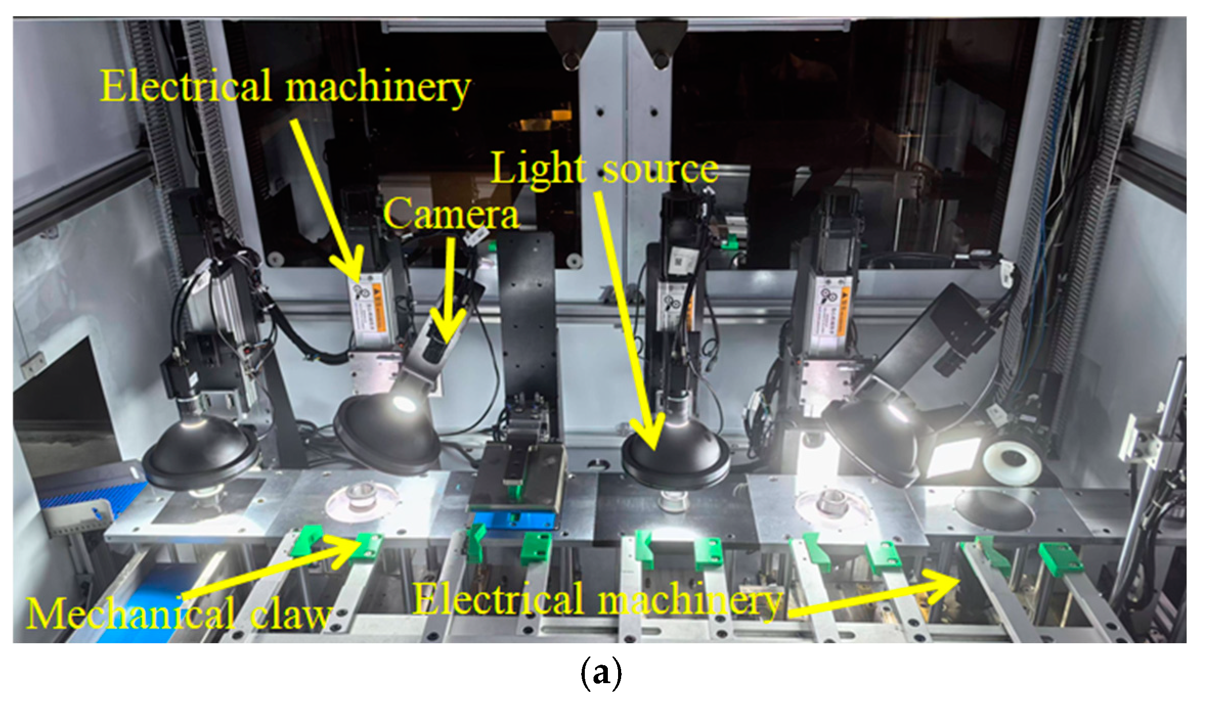
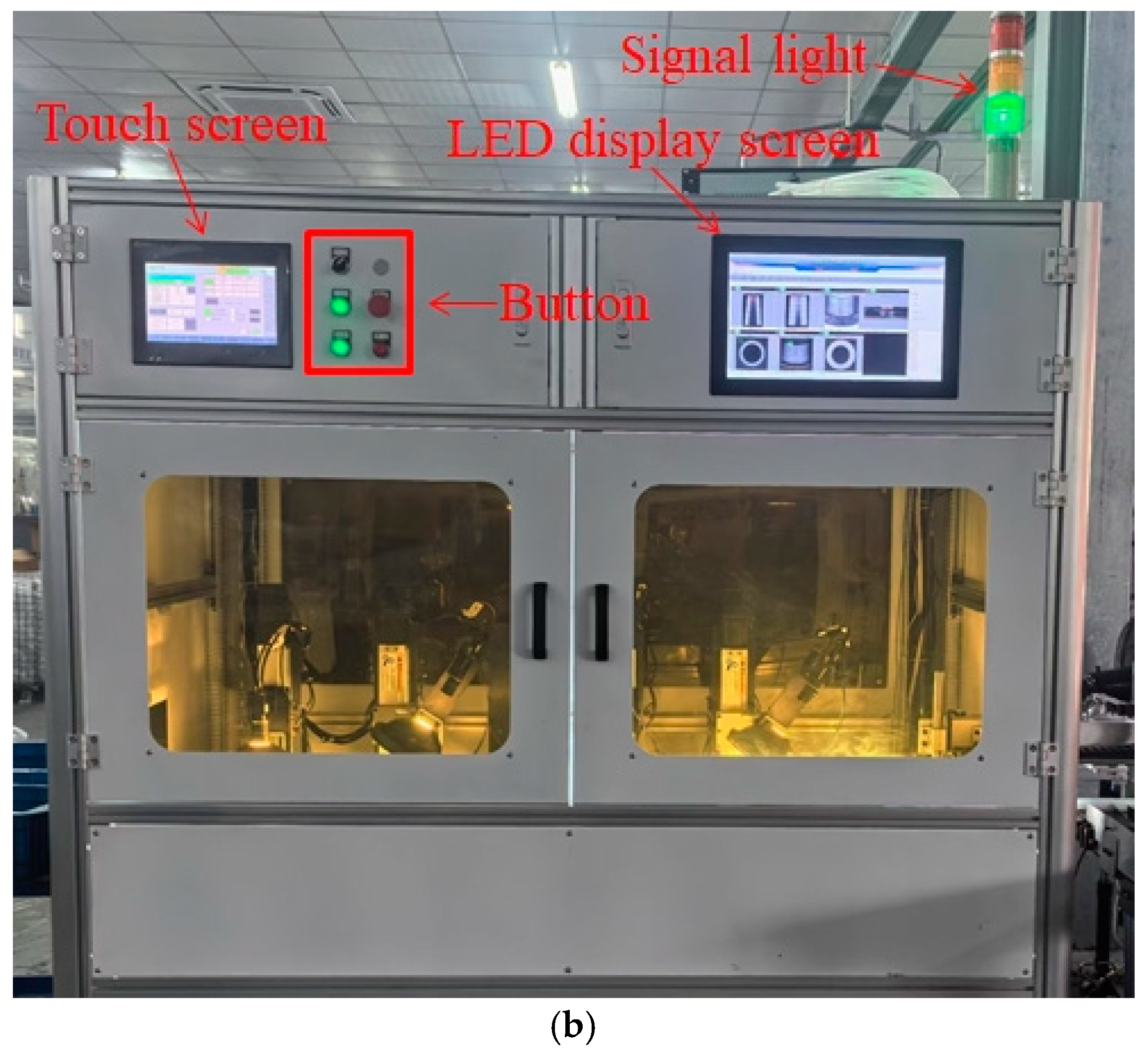
3. Bearing Surface Defect Detection Device

3.1. Principle of Bearing Surface Defect Detection Device

The overall appearance of the bearing surface defect detection device mainly includes a touch screen, an LED display screen, signal lights, and various buttons, as shown in Figure 1. The touch screen primarily shows the PLC control and monitors the overall operation of the machine; the LED display screen mainly shows the software interface operation, as well as the status of cameras at each station and their detection results; the buttons are mainly used to control the overall operation of the machine: the black button switches between manual and automatic modes, the green button is used for device initialization and startup, and the red button is used for device reset and emergency stop. Internally, the bearing defect detection device consists mainly of cameras, light sources, mechanical claw, and electrical machinery. Through PLC and sensor control, it triggers the industrial camera to take pictures, switches the light source, operates the electrical machinery, and controls the mechanical claw for gripping, thereby performing defect detection on the bearings and sorting them into qualified and unqualified categories.

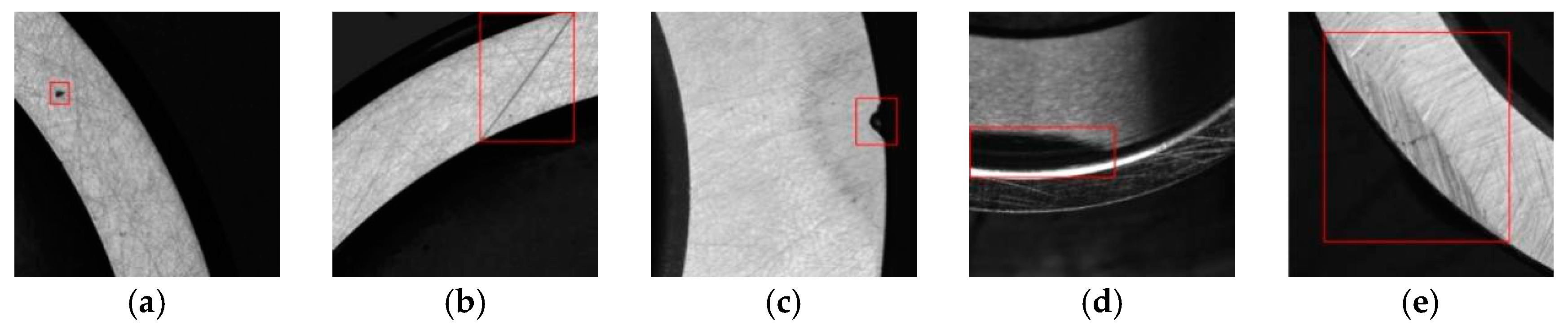
3.2. Types of Bearing Defects

During the operation of bearings, a variety of defects may arise, which can impact their performance and service life. Common defects include black spots, scratches, dents, material waste, and wear.

(1)

Black spots

The black spot defect, marked by a red square in Figure 2a, is typically caused by surface oxidation due to humid environmental conditions or uneven application of anti-rust oil. Defects larger than 0.5 mm × 0.5 mm need to be detected.

(2)

Scratches

The scratch defect, highlighted by a red square in Figure 2b, is often caused by improper assembly or incorrect handling during the turning process. Defects with a width greater than 0.1 mm and a length exceeding 1 mm need to be detected.

(3)

Dents

The dent defect, indicated by a red square in Figure 2c, is commonly caused by impact during transportation and installation. Defects larger than 0.5 mm × 0.5 mm need to be detected.

(4)

Material waste

The material waste defect, marked by a red square in Figure 2d, is typically caused by material quality issues during the manufacturing process or improper forging operations. Defects with a width greater than 0.1 mm and a length exceeding 0.5 mm need to be detected.

(5)

Wear

The wear defect, highlighted by a red square in Figure 2e, is typically caused by factors such as poor lubrication, improper assembly, overload operation, or excessive temperature. Defects larger than 0.5 mm × 0.5 mm need to be detected.

4. Algorithm Improvement

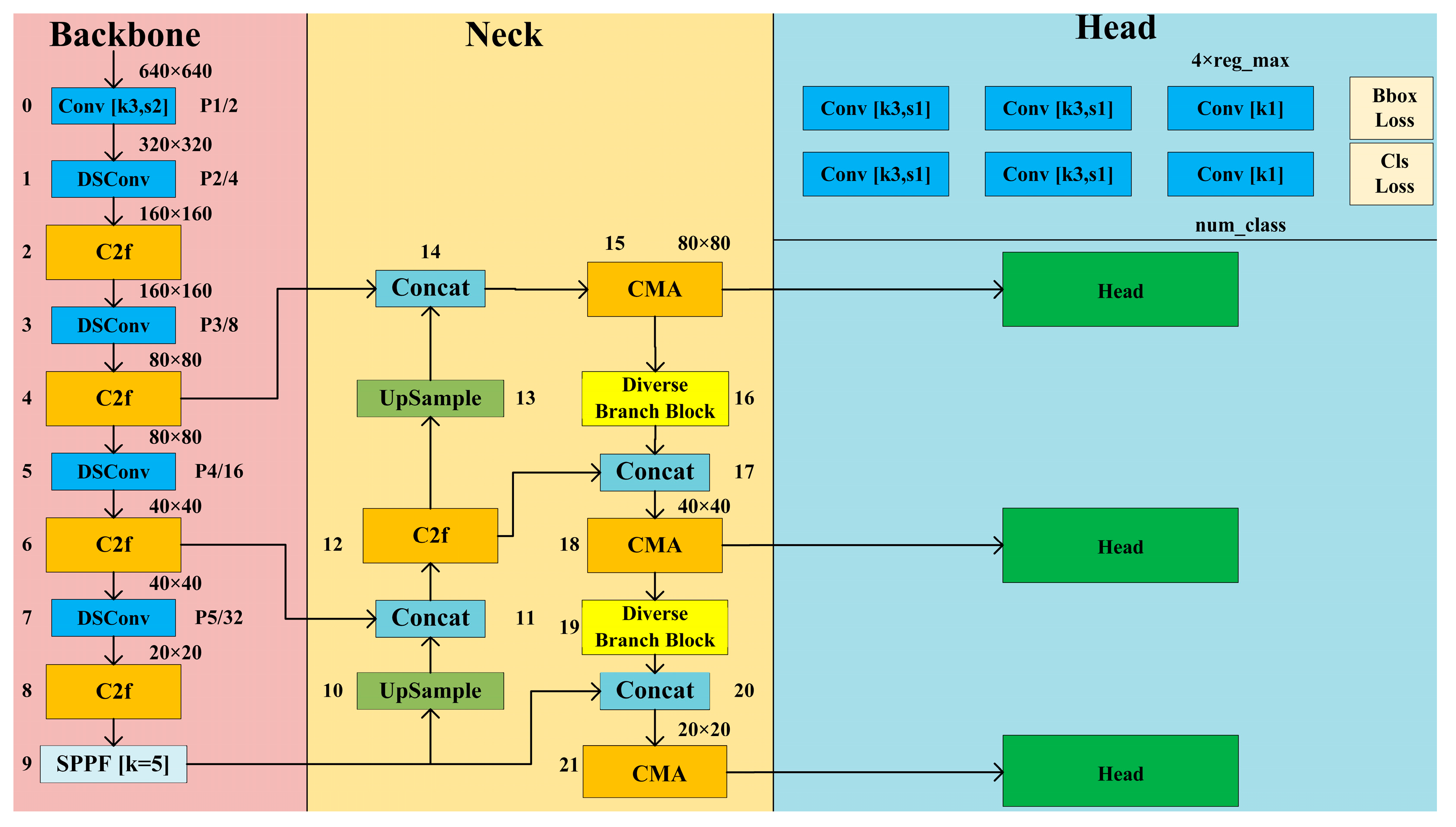
4.1. Yolov8s-DDC

YOLOv8, released by the Ultralytics team in January 2023, has demonstrated outstanding performance in tasks such as object detection, image segmentation, and pose estimation. It maintains the real-time detection capabilities of the YOLO series, achieving high frame rates even on lower hardware configurations. The model introduces improved multi-scale prediction techniques, allowing for better detection of objects of varying sizes. Additionally, it has optimized the adaptive adjustment of anchor boxes, enabling more accurate predictions of object positions and sizes.

YOLOv8 provides models in different sizes (N, S, M, L, X) to accommodate various deployment scenarios. Its architecture comprises three main components: Backbone, Neck, and Head. The Backbone uses the C2f module, which improves feature extraction through Bottleneck Blocks and SPPF modules. The Neck, positioned between the Backbone and Head, handles feature fusion and enhancement. The Head is responsible for generating the final detection outputs.

To address the complexity and diversity of bearing surface defects as well as the multi-scale challenges, this paper improves upon YOLOv8s by constructing the YOLOv8s-DDC architecture, as shown in Figure 3. This approach introduces Depthwise Separable Convolution into the Backbone to reduce computational complexity and the number of parameters while effectively capturing both spatial and channel information. Additionally, a Diverse Branch Block (DBB) is added to the Neck to strengthen feature representation. The DBB uses structural reparameterization by integrating diversified branches that handle different scales, enriching the feature space and improving detection efficiency, especially for high-resolution images. It also minimizes information loss and feature redundancy compared to traditional convolutions. Finally, a new module called CMA is introduced at the end of the Neck. This module incorporates the Monte Carlo Attention mechanism, which generates scale-invariant attention maps through stochastic sampling pooling. The mechanism is particularly beneficial for detecting small objects, which are often obscured or blurred in feature layers. Monte Carlo Attention improves small object detection by adaptively weighting important features.

By incorporating the Diverse Branch Block and CMA in the Neck network, the diversity of features and the network’s representational capability are enhanced while simultaneously optimizing the performance in small object detection. The Diverse Branch Block replaces the original convolutional layers, capturing information at different scales and levels, which improves the model’s adaptability to complex scenes and diverse objects. It optimizes parameter efficiency, reduces the total number of parameters, and maintains strong representational power. Overall, after introducing Depthwise Separable Convolution, Diverse Branch Block, and CMA, the network’s overall performance is significantly improved. Depthwise Separable Convolution reduces computational complexity and parameter count, the Diverse Branch Block enhances feature extraction diversity and expressiveness, and CMA optimizes small object detection through adaptive feature weighting.

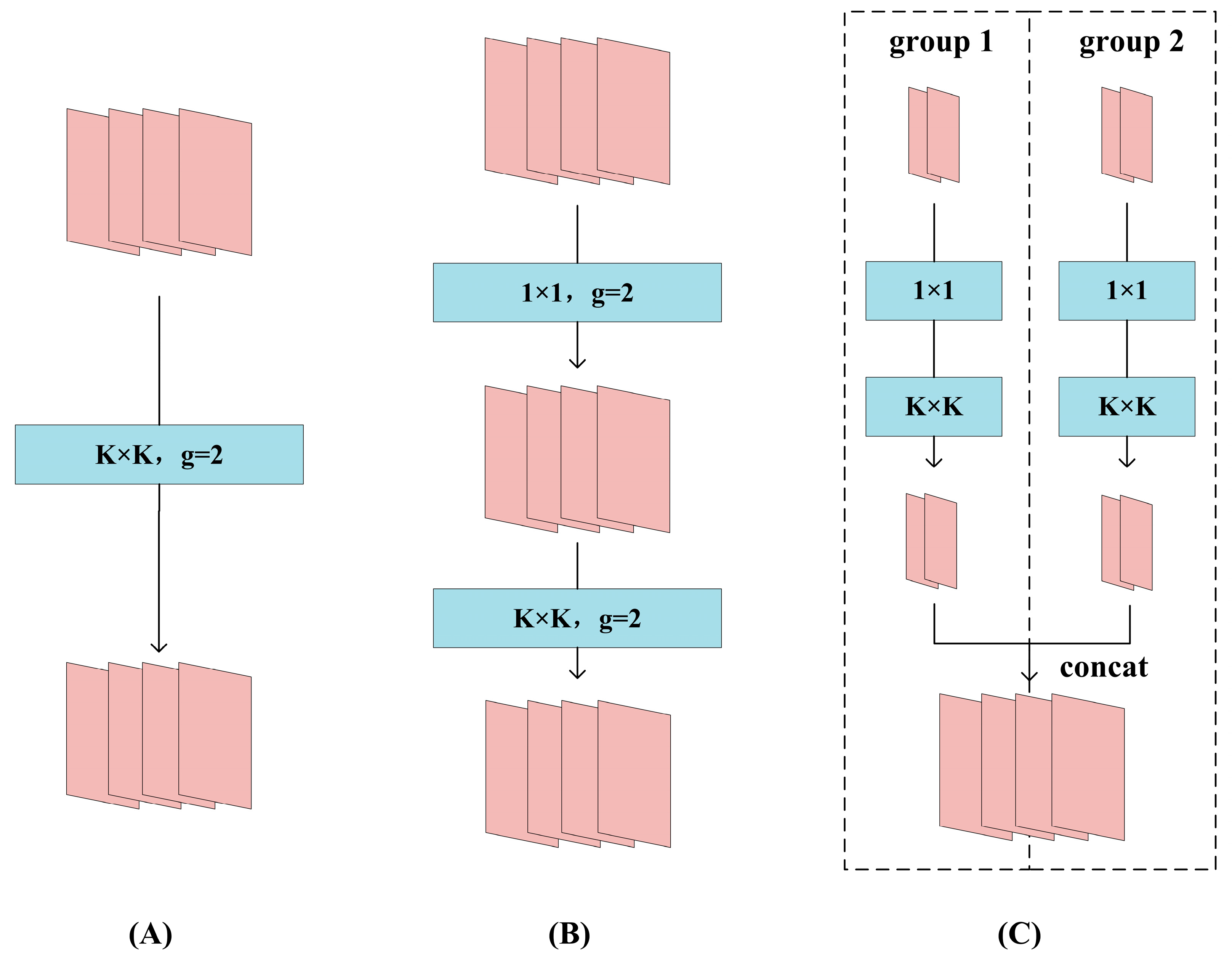
4.2. Depthwise Separable Convolution

Depthwise Separable Convolution (DSC) [35] is an efficient convolution operation in modern convolutional neural networks, particularly useful in resource-constrained environments. The structure of DSC, as shown in Figure 4, consists of two main steps:

(1) Depthwise Convolution: This process performs convolution independently on each channel of the input feature map. For each channel, a small convolution kernel (e.g., 3 × 3) is applied, effectively extracting spatial features. Since each channel is processed independently, the computational cost is relatively low.

(2) Pointwise Convolution: In this stage, a 1 × 1 convolution kernel is applied to the output of the depthwise convolution. The purpose of pointwise convolution is to combine features from different channels to generate a new output feature map. This approach allows the network to learn the relationships and interactions between channels.

In this paper, the convolution kernel size for depthwise convolution is 3 × 3 with a stride of 2, while the convolution kernel size for pointwise convolution is 1 × 1 with a stride of 2. The activation function used is GELU [36].

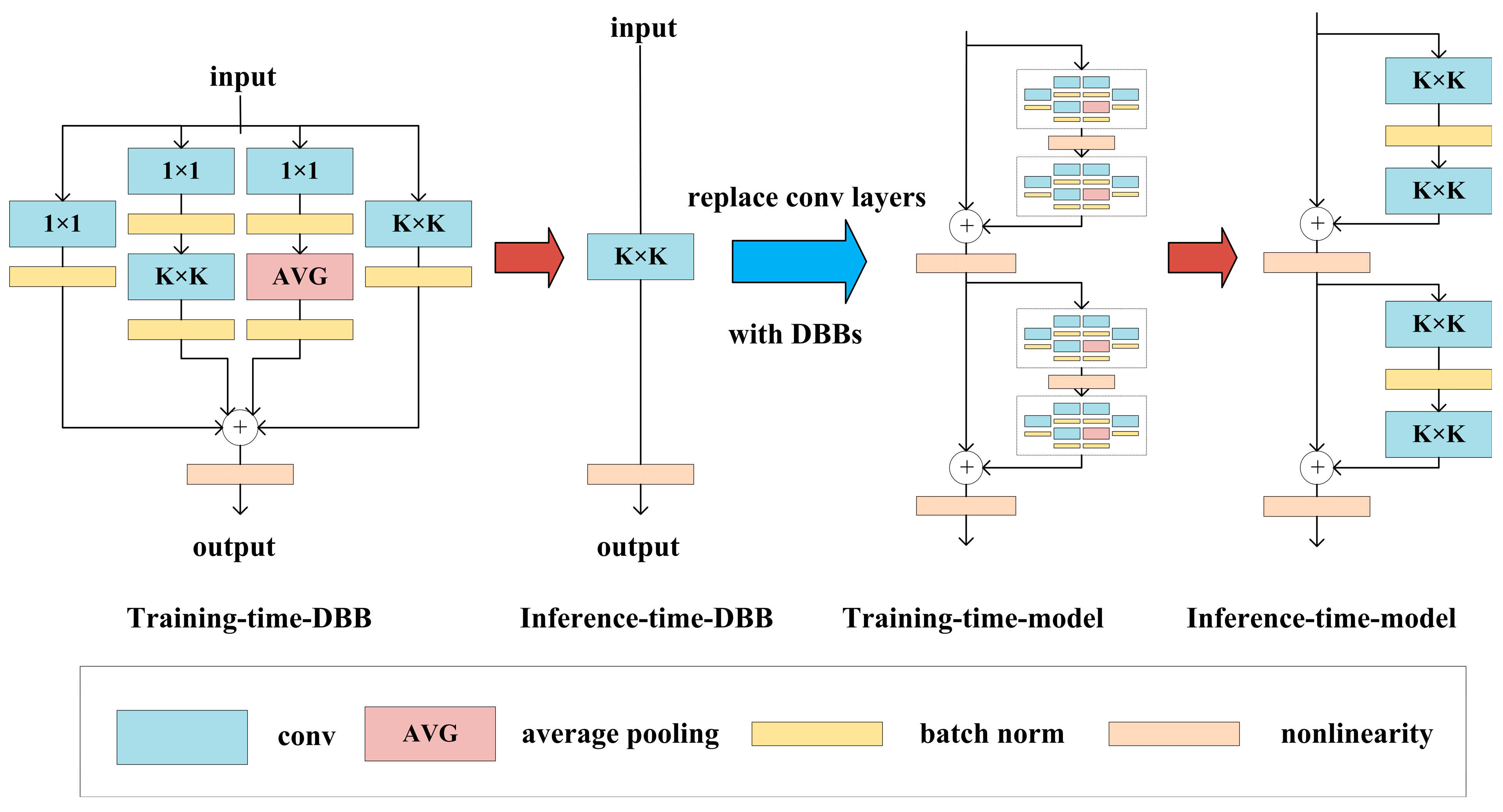
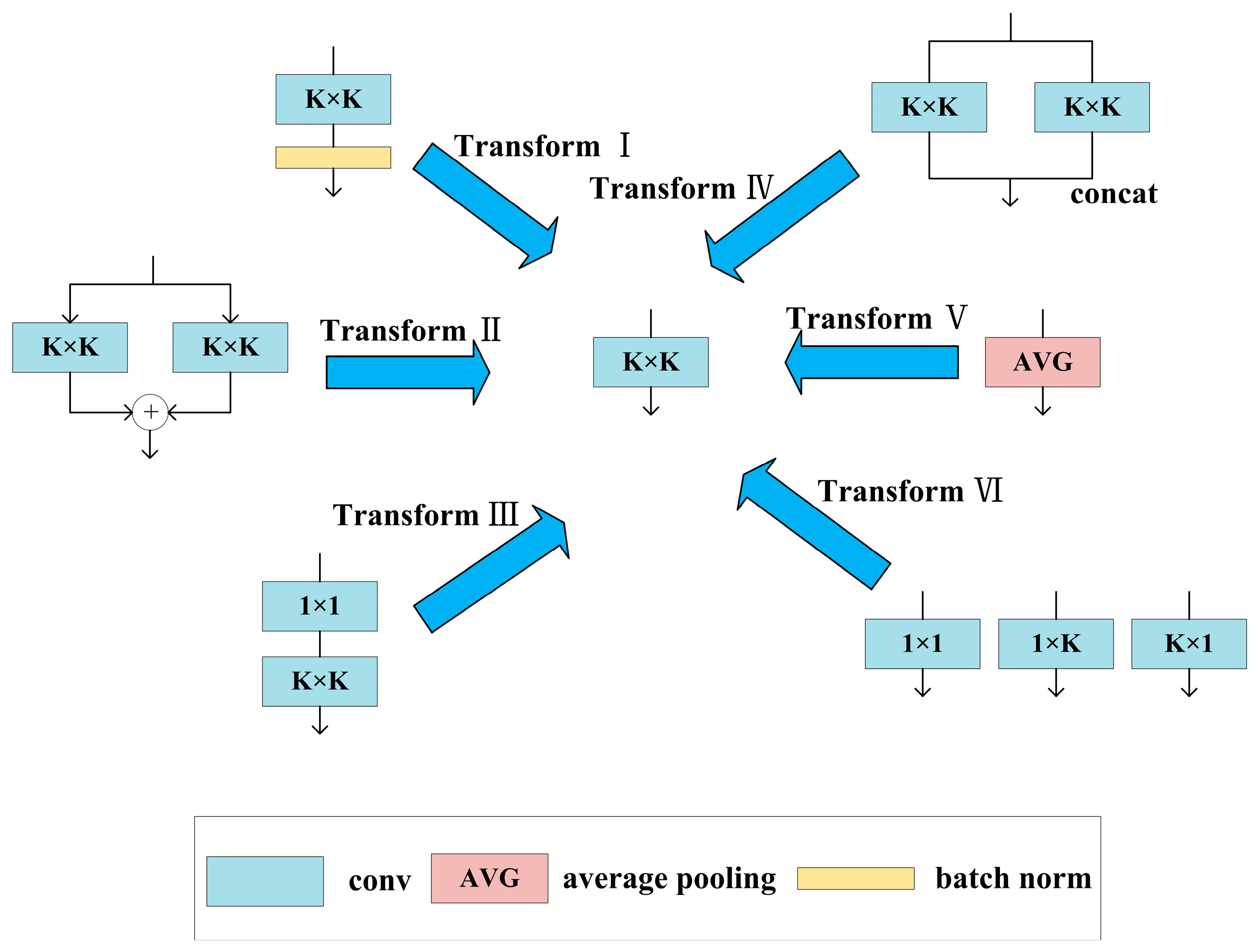
4.3. Diverse Branch Block

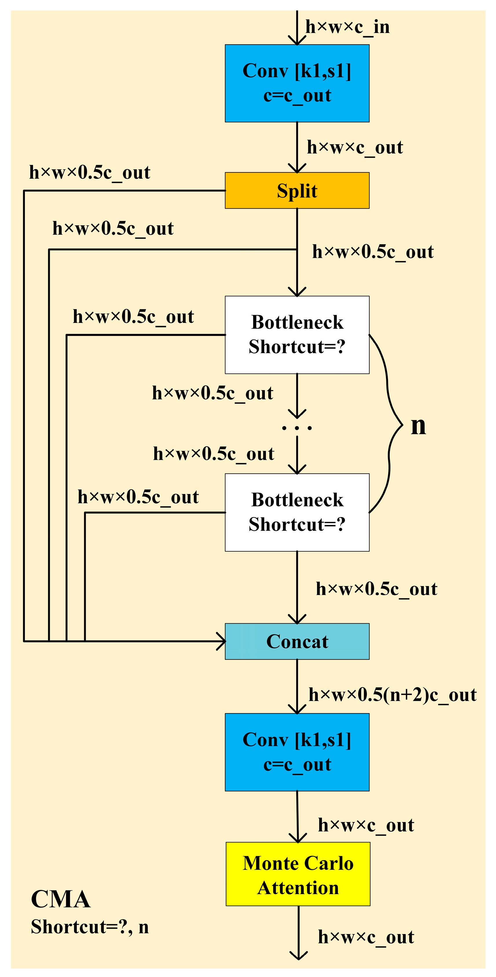
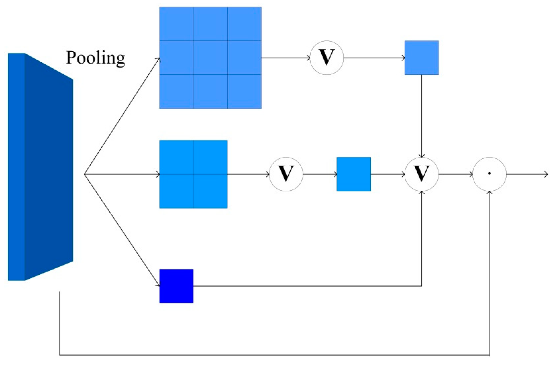
The basic principle of the Diverse Branch Block (DBB) [37] is to increase the complexity of the network during the training phase by introducing convolutional branches of different sizes and structures, thereby enhancing the feature representation capability. A representative design is shown in Figure 5.

We can summarize the fundamental principles into the following three points:

(1) Diverse branch structure: The Diverse Branch Block (DBB) integrates branches of varying scales and complexities, such as convolution kernels of different sizes and average pooling, to enhance the feature representation capability of individual convolutions. This diversity enables the network to simultaneously capture both local and global features, thereby enhancing the richness of the feature representations.

(2) Separation of Training and Inference: During training, the Diverse Branch Block (DBB) utilizes a complex branching structure to capture underlying data features effectively. However, during inference, these branches are simplified into a single convolutional layer, ensuring efficient computation. This approach strikes an optimal balance between performance and efficiency in both phases.

(3) Flexible Architecture Integration: The DBB can replace conventional convolutional layers and be seamlessly integrated into existing networks without modifying the overall architecture. This flexibility allows the DBB to enhance performance across various deep learning models without extensive reengineering.

As illustrated in Figure 5, during training (left side), the DBB consists of convolutional and average pooling layers of varying sizes, arranged in parallel and merged at the output. Once training is complete, these complex structures are transformed into a single convolutional layer for the model’s inference phase (right side), ensuring efficiency during inference. This transformation allows the Diverse Branch Block (DBB) to introduce micro-level structural complexity during training while maintaining the macro-level architecture, effectively enhancing the model’s performance.

The structure of the Diverse Branch Block (DBB) is designed to enhance the model’s feature extraction capability through diversified branches. These branches consist of convolutional layers, pooling layers, and other potential operations of varying sizes, which work in parallel to capture different feature representations. After training, these complex structures can be merged into a single convolutional layer, ensuring no additional computational burden during inference. This design allows the Diverse Branch Block (DBB) to directly replace existing convolutional layers, thereby improving the performance of the network architecture. As shown in Figure 6, six conversion methods are presented in detail to transform the DBB from the training phase into a conventional convolutional layer for the inference phase.

Among these, Transform I fuses convolutional layers with batch normalization to reduce model complexity; Transform II merges the outputs of convolutional layers with the same configuration to further simplify computation; Transform III combines sequential convolutional layers to improve feature extraction efficiency; Transform IV merges multiple convolutional layers through deep concatenation (Concat) to enhance feature diversity; Transform V integrates the average pooling (AVG) operation into the convolutional process to reduce computational burden and improve feature extraction capability; Transform VI combines convolutional layers of different scales to strengthen the model’s ability to capture multi-scale features.

Through these conversion methods, the Diverse Branch Block (DBB) is able to enhance the model’s performance and efficiency without increasing the computational cost during inference.

The Diverse Branch Block (DBB) employs a complex structure during the model training phase to fully leverage its diversity for enhanced feature extraction and learning capabilities. During the inference phase, the DBB is transformed into a simplified convolutional structure. This design effectively balances the high expressive power during training with computational efficiency during inference, ensuring that the model remains efficient while fully exploiting its learning potential.

As shown in Figure 7, one of the six methods is illustrated with an example. Assuming the input and output are 4-channel feature maps with a group number of g = 2, both the 1 × 1 and K × K convolutional layers are set to g = 2. During the conversion process, the layers are divided into g groups, Transform III is applied to each group, and Transform IV is used to concatenate the convolution kernels and biases.

In summary, the Diverse Branch Block (DBB) enhances the feature extraction capability of deep learning models by introducing diversified branch structures and flexible architectural integration. It achieves efficient conversion between training and inference, offering significant practical value.

4.4. CMA

We introduce a novel CMA module, shown in Figure 8, which builds on the C2f module and combines the Monte Carlo Attention (MCA) mechanism to improve feature representation. Specifically, the C2f module improves the diversity and richness of feature extraction by integrating information from multiple scales. The Monte Carlo Attention mechanism optimizes attention allocation by performing random sampling on the feature map. Using Monte Carlo methods, it automatically captures key spatial and channel information, enhancing the model’s focus on important regions. Embedding the Monte Carlo Attention (MCA) into the C2f module significantly improves the network’s ability to model complex image features. This is particularly useful for visual tasks with high noise or background interference, as the MCA module enables more precise focus on valuable regions. Overall, this approach enhances feature richness and improves the model’s accuracy and robustness across various tasks.

Monte Carlo Attention (MCA) generates scale-independent attention maps through a pooling operation based on random sampling. This approach allows the network to flexibly capture information across different scales, thereby improving its ability to recognize small objects. Specifically, MCA introduces randomness, reducing the dependency on specific scales and encouraging the model to learn richer feature representations. Compared to traditional attention mechanisms, MCA can automatically adjust its focus, enhancing the comprehensiveness of feature capture. Additionally, during training, random sampling aids in exploring the feature space, thus improving the model’s robustness and generalization ability.

The structure of Monte Carlo Attention (MCA) is shown in Figure 9. MCA (represented by the blue block) generates attention maps by randomly selecting a 1 × 1 attention map from pooled tensors at three different scales (3 × 3, 2 × 2, 1 × 1). In contrast to traditional methods like Squeeze-and-Excitation (SE), which rely on global average pooling to obtain a 1 × 1 output tensor and primarily focus on inter-channel dependencies, Monte Carlo Attention (MCA) excels in effectively utilizing cross-scale correlations. By combining features from three different scales (3 × 3, 2 × 2, 1 × 1) to compute the attention map, MCA overcomes the limitations of traditional methods and enhances long-range semantic dependencies.

Given an input tensor $x$, the attention map of Monte Carlo Attention (MCA) is denoted as $A_m\left(x\right)$, and the computation formula is expressed as Equation (1):

$$A_m\left(x\right)={\sum }_{i=1}^n{P}_1\left(x,i\right)f\left(x,i\right)$$

(1)

where $i$ represents the output size of the attention map and $f\left(x,i\right)$ denotes the average pooling function. The correlation probability $P_1\left(x,i\right)$ satisfies conditions $\sum _{i=1}^n{P}_1\left(x,i\right)=1$ and ${\prod }_{i=1}^n{P}_1\left(x,i\right)=0$, ensuring the generation of attention maps that are independent and generalizable. $n$ represents the number of output pooled tensors.

The Monte Carlo sampling method described in Equation (1) plays a crucial role in image processing and analysis. By randomly selecting correlation probabilities, this method enables the model to extract information from multiple dimensions, including local features (such as angles, edges, and colors) and contextual features (such as overall texture, spatial correlation, and color distribution). Specifically, the function of this formula is as follows:

(1) Enhancing the comprehensiveness of information extraction: Through randomization, Monte Carlo sampling can cover a broader feature space, ensuring that both local and global information diversity is thoroughly considered. This diversity is crucial for the analysis of complex images, especially when dealing with scenes that contain a variety of features.

(2) Improving the model’s adaptability: As this method can capture diverse visual information, the model exhibits greater robustness when confronted with variations and uncertainties. For instance, in natural scenes, factors such as lighting changes, object occlusions, or color variations may affect information extraction, and Monte Carlo sampling effectively addresses these challenges.

(3) Facilitating the understanding of complex data: By integrating both local and global information, Monte Carlo sampling aids in uncovering underlying patterns and structural relationships within images. This is of paramount importance for various applications, such as computer vision, image recognition, and scene understanding.

In summary, this approach not only enhances the diversity of information extraction but also improves the model’s robustness in complex image analysis. By integrating multi-dimensional information, Monte Carlo sampling provides a solid foundation for understanding complex visual content. It holds significant theoretical and practical value in enhancing image processing performance.

5. Experimental Verification

5.1. Dataset of Bearing Surface Defects

The various bearing surface defect images collected in actual industrial settings are shown in Figure 2, which primarily includes five types of defects: black spots, scratches, dents, material waste, and wear. The collection process is illustrated in Figure 1a. The bearings are conveyed to a designated position by a conveyor belt then gripped by a mechanical claw and moved to the center of the workstation. The electrical machinery drives the rotating disc, and the camera captures images during rotation. This process is repeated until the bearing reaches the final workstation, where an algorithm is used to differentiate between qualified and unqualified bearings.

The device collected bearing surface defect images with resolutions of 5472 × 3468 and 2024 × 2020, which were manually cropped and standardized to a size of 640 × 640. To address the issue of data imbalance, data augmentation techniques such as rotation, flipping, and cropping were applied to the training set. These operations were limited to the training set to ensure diversity within the training data and enhance the model’s generalization ability. The dataset was split into training, validation, and test sets, with 60% of the data used for training, 20% for validation, and 20% for testing. During the data augmentation process, we ensured that the number of samples for each defect type was as balanced as possible to improve the model’s ability to recognize different defect types. Meanwhile, no augmentation was applied to the validation and test sets to maintain their integrity and ensure unbiased evaluation results. As a result, the dataset was expanded to 5148 images. The number of images for each type of bearing surface defect after augmentation is shown in

Table 1. Number of bearing surface defect images for each type after augmentation.

	Black Spots	Scratches	Dents	Material Waste	Wear
Number	1049	1029	1023	1020	1027

. The dataset division is shown in

Table 2. Dataset partition table.

	Training Set	Verification Set	Test Set	Total Quantity
Black spots	626	205	218	1049
Scratches	593	211	225	1029
Dents	610	204	209	1023
Material waste	620	206	194	1020
Wear	639	204	184	1027

.

5.2. Experimental Setup and Performance Indicators

5.2.1. Experimental Setup

The experiments were conducted on a Linux Ubuntu operating system, with hardware configuration including an AMD EPYC 7642 processor (manufactured by Advanced Micro Devices, Inc. in Santa Clara, CA, USA) and an RTX 3090 GPU with 24 GB of VRAM. The software environment consists of Python 3.8.19, along with PyTorch 1.12.1 and CUDA 11.3, used for setting up and accelerating the deep learning framework. During training, the number of epochs was set to 200, the batch size was set to 8, the learning rate was set to 0.01, and the SGD optimizer was used. The input image size was standardized to 640 × 640. These experimental settings ensure that the model can be trained within a reasonable time frame given the available hardware resources while maintaining result stability and reproducibility.

5.2.2. Performance Indicators

The performance of the proposed algorithm is primarily evaluated using five metrics: precision, recall, mean average precision (mAP), frames per second (FPS), and giga floating point operations (GFLOPs).

Precision represents the proportion of actual positive samples among all samples predicted as positive, while recall denotes the proportion of correctly identified positive samples among all actual positive samples. The calculations for both metrics are given by Formulas (2) and (3), respectively.

$$P={\displaystyle \frac{TP}{TP+FP}}$$

(2)

$$\mathrm{R}={\displaystyle \frac{TP}{TP+FN}}$$

(3)

where, P represents precision, R represents recall, TP (true positive) refers to the samples that are predicted as positive and are actually positive, FP (false positive) refers to the samples that are predicted as positive but are actually negative, and FN (false negative) refers to the samples that are predicted as negative but are actually positive.

Mean Average Precision (mAP) measures the overall detection performance of the trained model across all classes. The calculation formula is given by Equation (4).

$$\mathrm{m}\mathrm{A}\mathrm{P}={\displaystyle \frac{{\sum }_{i=1}^K{AP}_i}{K}}$$

(4)

where AP represents the average precision for a single class and K denotes the number of classes.

Frames per second (FPS) is commonly used to evaluate the performance of a model in real-time object detection tasks. Specifically, it refers to the number of image frames the model can process and predict per second. The calculation formula is given by Equation (5).

$$\mathrm{F}\mathrm{P}\mathrm{S}={\displaystyle \frac{1}{Processing time per frame}}$$

(5)

where “Processing time per frame” refers to the time taken to process each individual frame.

The calculation formula for FPS in YOLO is given by Equation (6), and typically, 1 s is converted to 1000 milliseconds for the calculation.

$$\mathrm{F}\mathrm{P}\mathrm{S}={\displaystyle \frac{1000}{pre-process+inference+NMS}}$$

(6)

where “pre-process” refers to the image preprocessing time, “inference” represents the inference speed, and “NMS” stands for the post-processing time.

The number of floating-point operations (GFLOPs) is primarily used to measure the complexity of an algorithm/model. A lower GFLOPs value indicates higher computational efficiency of the model.

5.3. Ablation Experiment

In this experiment, three improvements were made to YOLOv8. To validate the effectiveness of the network improvements, we conducted ablation experiments, as shown in

Table 3. Ablation experiment.

	DSC	DBB	MCA	mAP	FPS	Parameters	GFlOPs
Yolov8s				95.4%	128	11.13 M	28.7
DSC	√			95.9%	131	9.74 M	25.1
DBB		√		96%	113	12.11 M	29.9
CMA			√	96%	124	11.81 M	28.4
DSC + DBB	√	√		96.3%	115	10.72 M	26.6
DSC + CMA	√		√	96.5%	123	10.43 M	25.7
DBB + CMA		√	√	96.5%	105	12.8 M	30.5
Ours	√	√	√	96.9%	106	11.41 M	26.6

. In the table, √ indicates the adoption of the corresponding module; DSC stands for Depthwise Separable Convolution, and DBB represents Diverse Branch Block.

According to Table 3, the initial YOLOv8s model achieves an mAP of 95.4% and FPS of 128 frames per second. After adding DSC to the Backbone network, the mAP increases to 95.9%, FPS rises to 131 frames per second, and the number of parameters decreases to 9.74 M, thus improving both detection accuracy and efficiency. When DBB is introduced into the Neck network, the mAP further increases to 96%. With the addition of CMA at the end of the Neck, the mAP rises to 96% while GFLOPs decrease to 28.4. When the aforementioned improvements are applied in pairs, the mAP increases by 0.9%, 1.1%, and 1.1%, respectively. When all the improvements are combined, the mAP increases by 1.5%, and the number of parameters remains nearly the same as the original model. Although the FPS decreases to 106 frames per second, the GFLOPs also drop to 26.6. This indicates that, despite the decline in frame rate, computational efficiency has not significantly decreased. The model maintains a balance between detection accuracy and computational efficiency, which is still capable of meeting practical industrial demands. This is especially important in applications where high precision is critical, such as industrial defect detection, autonomous driving, and intelligent surveillance, where accuracy is often the primary concern. In these scenarios, a slight reduction in FPS is acceptable, particularly when processing high-resolution images or complex scenes. Therefore, we believe that the algorithm’s balance between detection accuracy and computational efficiency is well suited to meet the requirements of real-world industrial applications.

5.4. Feature Visualization Analysis

As shown in Figure 10, the performance of the CMA and DBB modules in the visualization of characteristics related to black spots, scratches, dents, material waste, and wear reveals their advantages and limitations in detecting different types of defects. The analysis is as follows:

(1) The CMA module excels in feature extraction for dents and material waste, efficiently identifying these defects and enhancing the sensitivity and accuracy of the detection process. This capability allows for the timely detection of potential issues that may impact product quality.

(2) In contrast, the DBB module demonstrates outstanding performance in scratch detection, accurately identifying and locating surface scratches through advanced algorithms. This precision is crucial for quality control and helps reduce product losses due to scratches.

(3) Regarding black spot detection, both the CMA and DBB modules perform similarly, indicating their effectiveness in handling this particular defect type.

The CMA and DBB modules exhibit distinct advantages in feature detection, each performing differently with respect to various types of defects.

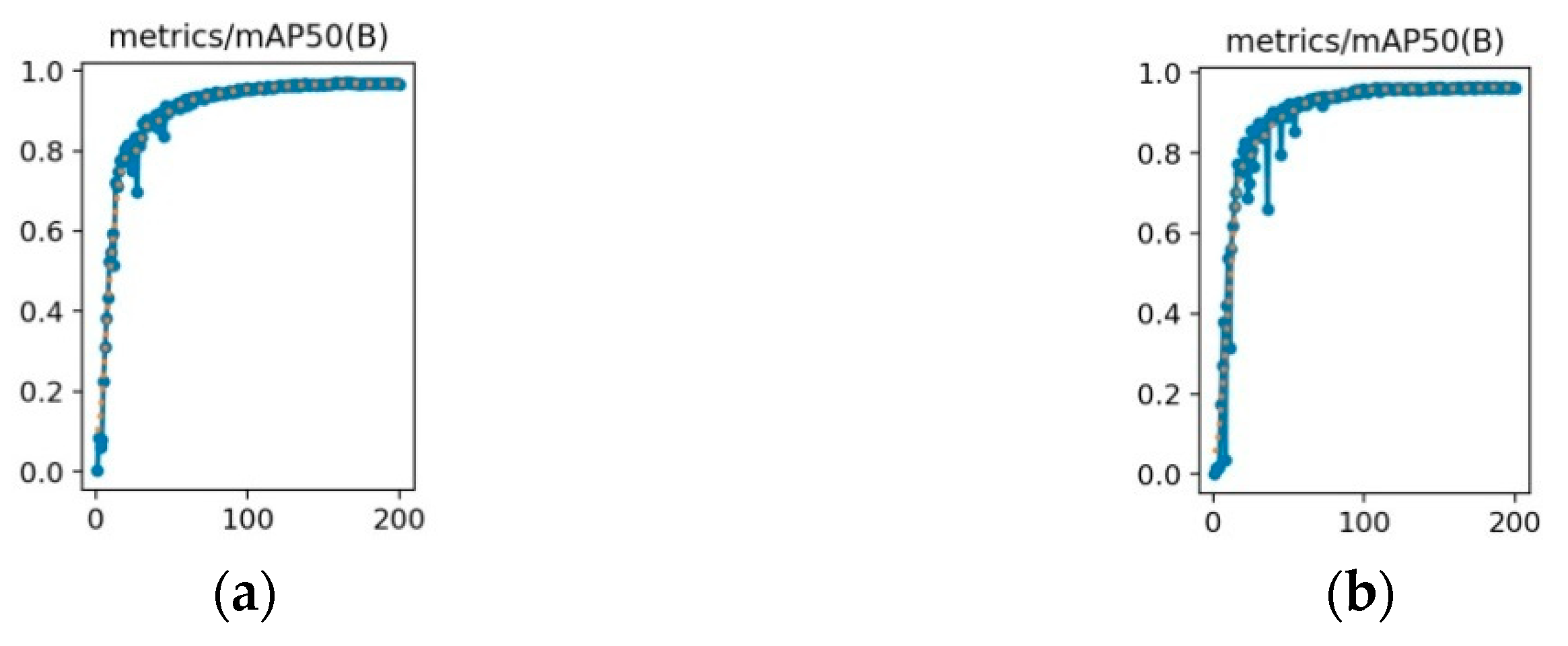
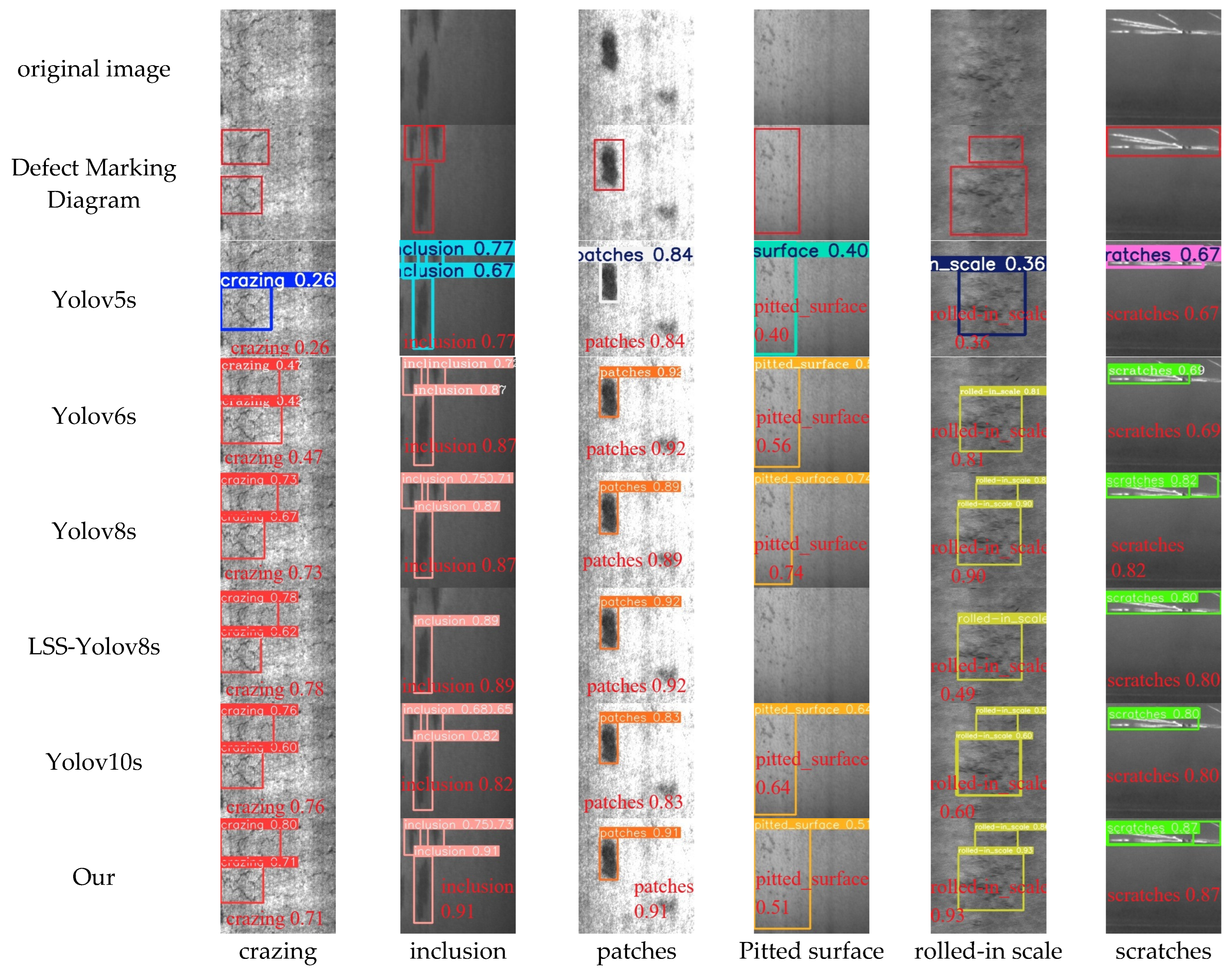
5.5. Experimental Results and Comparative Experiments

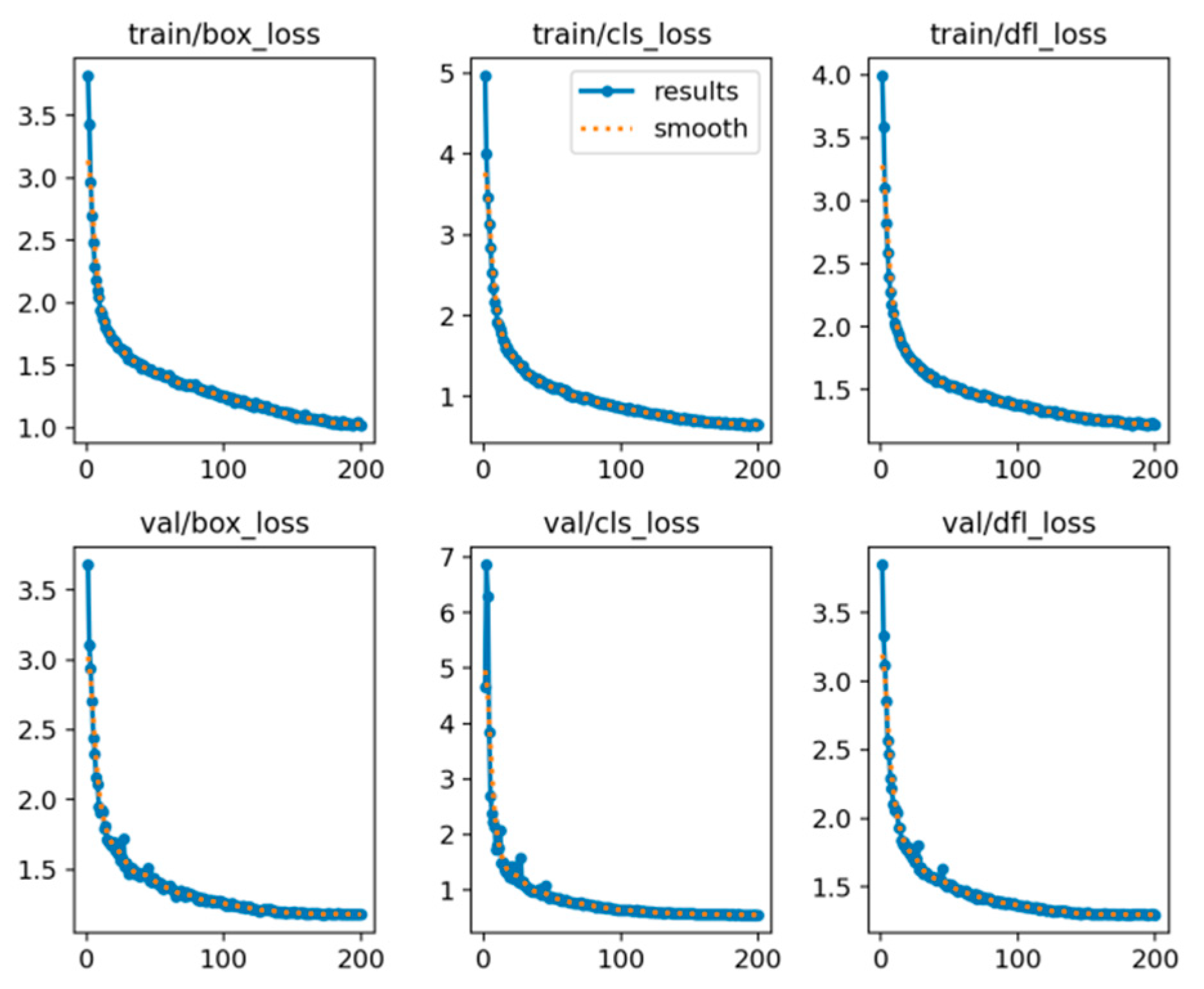
The training and validation losses during the training process of this experiment are shown in Figure 11. The horizontal axis represents “Epochs”, indicating the number of training iterations, while the vertical axis represents “Loss”, indicating the value of the loss function. It can be observed that both the training loss and validation loss rapidly converge within the first approximately 50 epochs and fully converge by epoch 200.

The three sets of graphs in Figure 10 represent different types of losses:

(1)

train/box_loss: This indicates the loss for bounding box prediction during training, reflecting the model’s error in localizing target objects.

(2)

train/cls_loss: This represents the classification loss during training, reflecting the model’s error in classifying target categories.

(3)

train/dfl_loss: This denotes the distribution focal loss during training, which optimizes the distribution prediction in object detection.

(4)

val/box_loss, val/cls_loss, val/dfl_loss: These represent the corresponding losses on the validation set, used to evaluate the model’s performance on unseen data.

The rapid decrease in both training and validation losses within the first 50 epochs indicates that the model quickly learns and adapts to the data. By epoch 200, the losses stabilize, suggesting that the model has been sufficiently trained and has reached a good state of convergence.

The experimental results are shown in Figure 12. It can be observed that the experimental accuracy gradually improves with the increase in training iterations, starting to converge around the 150th iteration, and fully converging by the 200th iteration.

To further validate the rationality of the network model design, a comparison was made with the current mainstream object detection algorithms: Yolov5, Yolov6 [38], Yolov8, LSS-Yolov8, and Yolov10 [39]. The detection performance comparison is illustrated in Figure 13, and the comparative experiments are shown in

Table 4. Comparative experiments with related Yolo models.

	Yolov5s	Yolov6s	Yolov8s	LSS-Yolov8s	Yolov10s	Our
Black spots	95.4%	93.5%	92.9%	82.9%	91.2%	96.7%
Scratches	96.2%	99%	97.3%	92.3%	94.5%	98.5%
Dents	88.4%	84.9%	88.5%	87%	86.9%	90.4%
Material waste	98.5%	98.4%	99.5%	99.5%	99%	99.5%
Wear	93.5%	95.8%	98.6%	98.5%	97.4%	99.5%
P	92.5%	90.4%	94.9%	95.6%	91.2%	96.8%
R	89.9%	86%	92.4%	85.6%	87.2%	93.6%
mAP	94.4%	94.3%	95.4%	92%	93.8%	96.9%
FPS	122	115	128	113	80	106

.

In this study, we randomly selected one image from each defect category and performed detection using different object detection algorithms. The results are shown in Figure 13. In which hb represents black spots, hs represents scratches, kp represents dents, lf represents material waste, and ms represents eear. Our improved network demonstrates superior performance in detection accuracy across all defect types, generally outperforming other object detection algorithms. This result indicates that our improvements effectively enhance the network’s detection capabilities.

As shown in Table 4, our improved algorithm, Yolov8s-DDC, achieves a 2.5%, 2.6%, 1.5%, 4.9%, and 3.1% increase in mAP compared to other Yolo series object detection algorithms. Compared to the original Yolov8 model, mAP is improved by 1.5%, with detection accuracy for black spot and dent defects increasing by 3.8% and 1.9%, respectively. Additionally, precision and recall are enhanced by 1.9% and 1.2%, respectively. Although the FPS slightly decreased, the improved algorithm still meets the accuracy and efficiency requirements for industrial applications.

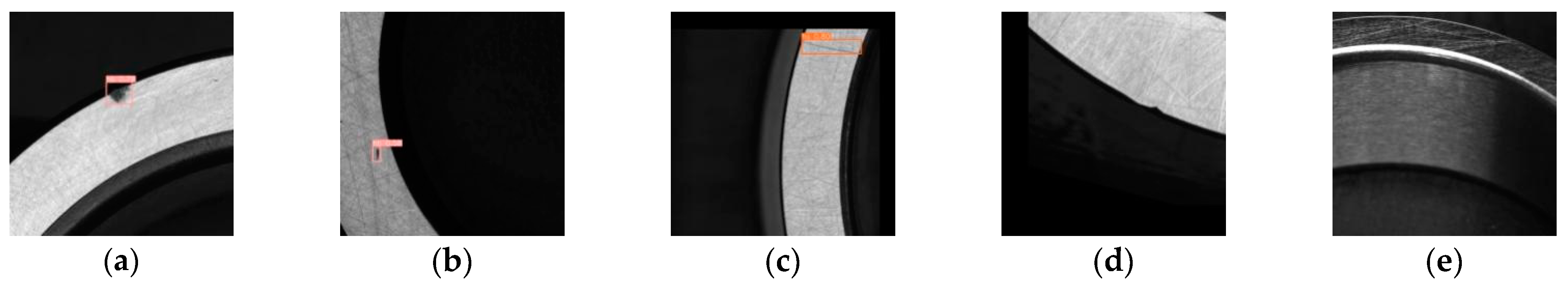
5.6. Causes of False Positives and False Negatives

As shown in Figure 14, during actual industrial field inspections, false positives and false negatives in bearing detection often occur. In Figure 14a, wear is misidentified as black spots. In Figure 14b,c, scratches are missed. In Figure 14d, dents are not detected, and in Figure 14e, material waste is overlooked. The specific reasons are as follows:

(1) During the bearing production process, the use of cleaning oil may result in oil droplets and impurities remaining on the bearing surface, which significantly interferes with the detection of surface defects, particularly in the identification of black spot defects. Therefore, when conducting defect detection, it is essential to consider factors such as lighting methods, light source color, and camera models. Additionally, a blower should be used to remove surface impurities or evenly distribute the oil droplets to prevent them from being misidentified as black spot defects.

(2) The depth of scratch defects is difficult to detect using a 2D camera, which may lead to misjudgments. Therefore, we have strengthened communication with the company personnel and refined the defect standards to minimize the occurrence of false positives.

(3) Different lighting methods may cause some defective bearings to be misjudged as defect-free, thereby affecting the accuracy of detection. In this experiment, bowl lighting and ring lighting were primarily used to minimize this effect.

5.7. Detection Results of the Public Datasets

To further evaluate the performance of the algorithm proposed in this paper, comparative experiments were conducted on the Northeastern University hot-rolled strip steel surface defect dataset. This dataset consists of 1800 images, divided into six defect categories: crazing, inclusion, patches, pitted surface, rolled-in scale, and scratches. The dataset was split into training, validation, and test sets in a 6:2:2 ratio. In the experiments, performance comparisons were made based on the YOLOv5, YOLOv6, YOLOv8, LSS-Yolov8s, and YOLOv10 models. The detection results of the experiment are shown in Figure 15, and a detailed summary of the comparative experiment data is provided in

Table 5. Comparative experiments with relevant YOLO models on the public dataset.

	Yolov5s	Yolov6s	Yolov8s	LSS-Yolov8s	Yolov10s	Our
crazing	38.7%	35.8%	42.9%	37.8%	35%	42.3%
inclusion	77.9%	79.4%	84.5%	59.5%	79.4%	84.5%
patches	89.8%	90.3%	94.2%	63.8%	88.7%	93.8%
Pitted surface	78%	82.9%	89.7%	83.1%	73.4%	84.2%
rolled-in scale	49.5%	56.2%	60.4%	54.1%	55.3%	65.6%
scratches	92.9%	95.3%	84.9%	73.7%	80.8%	90.3%
mAP	71.1%	73.3%	76.1%	62%	68.8%	76.8%
FPS	115	113	135	110	76	102

.

As shown in Figure 15 and Table 5, the improved Yolov8s-DDC algorithm demonstrates a clear advantage over the original Yolov8 model and also achieves significant improvements when compared to other detection algorithms. This indicates that the proposed Yolov8s-DDC algorithm is not only effective but also highly practical.

6. Conclusions

To address the complexity and diversity in bearing surface defect detection, this paper proposes an improved defect detection model, Yolov8s-DDC. By incorporating depthwise separable convolutions into the Backbone network, the model reduces computational complexity and the number of parameters, effectively enhancing feature extraction efficiency. Additionally, the introduction of a diversified branching module in the Neck network promotes a richer feature representation, enabling the network to capture feature information from different dimensions, thereby strengthening the overall detection capability. Furthermore, the proposed CMA, which combines the Monte Carlo attention mechanism, specifically optimizes the recognition of small targets, improving the detection performance of important features. We conducted extensive experiments on a bearing surface defect dataset collected from bearing enterprises to validate the effectiveness of the Yolov8s-DDC algorithm. The experimental results show that the algorithm achieves an average precision (mAP) of 96.9% and a detection speed of 106 frames per second (FPS). Compared to current mainstream object detection algorithms, Yolov8s-DDC improves accuracy by 1.5%, fully meeting the demands of industrial defect detection and demonstrating excellent application prospects. Additionally, experiments on the Northeastern University hot-rolled strip steel surface defect dataset also show performance improvements, with the final mAP reaching 76.8%. In future research, the performance of the network model can be further enhanced by introducing new networks and modules, or by designing new mechanical structures to mitigate the impact of factors such as oil droplets, impurities, and lighting. Additionally, by optimizing threshold settings, further reducing the influence of external interference factors, and expanding the dataset to better simulate complex industrial inspection scenarios, the robustness and accuracy of the model can be improved.

References

1. Redmon, J.; Divvala, S.; Girshick, R.; Farhadi, A. You only look once: Unified, real-time object detection. In Proceedings of the 2016 IEEE Conference on Computer Vision and Pattern Recognition, Las Vegas, NV, USA, 27–30 June 2016. [Google Scholar]
2. Liu, W.; Anguelov, D.; Erhan, D.; Szegedy, C.; Reed, S.; Fu, C.-Y.; Berg, A.C. Ssd: Single shot multibox detector. In Proceedings of the Computer Vision–ECCV 2016: 14th European Conference, Amsterdam, The Netherlands, 11–14 October 2016; pp. 21–37. [Google Scholar]
3. Girshick, R.; Donahue, J.; Darrell, T.; Malik, J. Rich feature hierarchies for accurate object detection and semantic segmentation. In Proceedings of the 2014 IEEE Conference on Computer Vision and Pattern Recognition, Columbus, OH, USA, 23–28 June 2014; pp. 580–587. [Google Scholar]
4. Ren, S.; He, K.; Girshick, R.; Sun, J. Faster R-CNN: Towards real-time object detection with region proposal networks. IEEE Trans. Pattern Anal. Mach. Intell. 2016, 39, 1137–1149. [Google Scholar] [CrossRef] [PubMed]
5. He, K.; Gkioxari, G.; Dollár, P.; Girshick, R. Mask r-cnn. In Proceedings of the 2017 IEEE International Conference on Computer Vision, Venice, Italy, 22–29 October 2017. [Google Scholar]
6. Liang, Y.; Xu, K.; Zhou, P. Mask gradient response-based threshold segmentation for surface defect detection of milled aluminum ingot. Sensors 2020, 20, 4519. [Google Scholar] [CrossRef] [PubMed]
7. Zhang, E.; Ma, Q.; Chen, Y.; Duan, J.; Shao, L. EGD-Net: Edge-guided and differential attention network for surface defect detection. J. Ind. Inf. Integr. 2022, 30, 100403. [Google Scholar] [CrossRef]
8. Zhang, J.; Guo, Z.; Jiao, T.; Wang, M. Defect detection of aluminum alloy wheels in radiography images using adaptive threshold and morphological reconstruction. Appl. Sci. 2018, 8, 2365. [Google Scholar] [CrossRef]
9. Cheng, B.; Li, B.; Ye, L. Defect detection of photovoltaic panel based on morphological segmentation. In Proceedings of the MIPPR 2023: Automatic Target Recognition and Navigation, Wuhan, China, 10–12 November 2023. [Google Scholar]
10. Zhou, P.; Zhou, G.; Li, Y.; He, Z.; Liu, Y. A hybrid data-driven method for wire rope surface defect detection. IEEE Sens. J. 2020, 20, 8297–8306. [Google Scholar] [CrossRef]
11. Hua, J.; Zhiquan, W. Resolving mode mixing in wheel–rail surface defect detection using EMD based on binary time scale. Meas. Sci. Technol. 2023, 35, 035015. [Google Scholar] [CrossRef]
12. Lan, S.; Li, J.; Hu, S.; Fan, H.; Pan, Z. A neighbourhood feature-based local binary pattern for texture classification. Vis. Comput. 2024, 40, 3385–3409. [Google Scholar] [CrossRef]
13. Wang, H.; Zhang, J.; Tian, Y.; Chen, H.; Sun, H.; Liu, K. A simple guidance template-based defect detection method for strip steel surfaces. IEEE Trans. Ind. Inform. 2018, 15, 2798–2809. [Google Scholar] [CrossRef]
14. Zhou, J.; Liu, Y.; Zhang, X.; Yang, Z. Multi-view based template matching method for surface defect detection of circuit board. J. Phys. Conf. Ser. 2021, 1983, 012063. [Google Scholar] [CrossRef]
15. Pastor-López, I.; Sanz, B.; de la Puerta, J.G.; Bringas, P.G. Surface defect modelling using co-occurrence matrix and fast fourier transformation. In Proceedings of the Hybrid Artificial Intelligent Systems: 14th International Conference, HAIS 2019, León, Spain, 4–6 September 2019. Proceedings 14. [Google Scholar]
16. Wang, F.-l.; Zuo, B. Detection of surface cutting defect on magnet using Fourier image reconstruction. J. Cent. South Univ. 2016, 23, 1123–1131. [Google Scholar] [CrossRef]
17. Rostami, B.; Shanehsazzadeh, F.; Fardmanesh, M. Fast fourier transform based NDT approach for depth detection of hidden defects using HTS rf-SQUID. IEEE Trans. Appl. Supercond. 2018, 28, 1–6. [Google Scholar] [CrossRef]
18. Yang, Z.; Zhang, M.; Chen, Y.; Hu, N.; Gao, L.; Liu, L.; Ping, E.; Song, J.I. Surface defect detection method for air rudder based on positive samples. J. Intell. Manuf. 2024, 35, 95–113. [Google Scholar] [CrossRef]
19. Zhang, Q.; Lai, J.; Zhu, J.; Xie, X. Wavelet-guided promotion-suppression transformer for surface-defect detection. IEEE Trans. Image Process. 2023, 32, 4517–4528. [Google Scholar] [CrossRef]
20. Liu, H.; Ma, R.; Li, Y. Asphalt Pavement Image Segmentation Method Based on Optimized Markov Random Field. In Proceedings of the 2021 6th International Conference on Transportation Information and Safety (ICTIS), Wuhan, China, 22–24 October 2021. [Google Scholar]
21. Xu, J.; Zuo, Z.; Wu, D.; Li, B.; Li, X.; Kong, D. Bearing Defect Detection with Unsupervised Neural Networks. Shock. Vib. 2021, 2021, 9544809. [Google Scholar] [CrossRef]
22. Wu, Y.; Lu, Y. An intelligent machine vision system for detecting surface defects on packing boxes based on support vector machine. Meas. Control. 2019, 52, 1102–1110. [Google Scholar] [CrossRef]
23. Ghiasi, R.; Khan, M.A.; Sorrentino, D.; Diaine, C.; Malekjafarian, A. An unsupervised anomaly detection framework for onboard monitoring of railway track geometrical defects using one-class support vector machine. Eng. Appl. Artif. Intell. 2024, 133, 108167. [Google Scholar] [CrossRef]
24. Kumar, A.; Zhou, Y.; Gandhi, C.; Kumar, R.; Xiang, J. Bearing defect size assessment using wavelet transform based Deep Convolutional Neural Network (DCNN). Alex. Eng. J. 2020, 59, 999–1012. [Google Scholar] [CrossRef]
25. Lu, M.; Mou, Y. Bearing defect classification algorithm based on autoencoder neural network. Adv. Civ. Eng. 2020, 2020, 6680315. [Google Scholar] [CrossRef]
26. Lei, L.; Sun, S.; Zhang, Y.; Liu, H.; Xie, H. Segmented embedded rapid defect detection method for bearing surface defects. Machines 2021, 9, 40. [Google Scholar] [CrossRef]
27. Ping, Z.; Chuangchuang, Z.; Gongbo, Z.; Zhenzhi, H.; Xiaodong, Y.; Shihao, W.; Meng, S.; Bing, H. Whole surface defect detection method for bearing rings based on machine vision. Meas. Sci. Technol. 2022, 34, 015017. [Google Scholar] [CrossRef]
28. Jia, H.; Zhou, H.; Chen, Z.; Gao, R.; Lu, Y.; Yu, L. Research on Bearing Surface Scratch Detection Based on Improved YOLOV5. Sensors 2024, 24, 3002. [Google Scholar] [CrossRef] [PubMed]
29. Zhao, Y.; Chen, B.; Liu, B.; Yu, C.; Wang, L.; Wang, S. GRP-YOLOv5: An improved bearing defect detection algorithm based on YOLOv5. Sensors 2023, 23, 7437. [Google Scholar] [CrossRef] [PubMed]
30. Wang, Y.; Song, Z.; Abdullahi, H.S.; Gao, S.; Zhang, H.; Zhou, L.; Li, Y. A Lightweight Detection Algorithm for Surface Defects in Small-Sized Bearings. Electronics 2024, 13, 2614. [Google Scholar] [CrossRef]
31. Liu, M.; Zhang, M.; Chen, X.; Zheng, C.; Wang, H. YOLOv8-LMG: An Improved Bearing Defect Detection Algorithm Based on YOLOv8. Processes 2024, 12, 930. [Google Scholar] [CrossRef]
32. Nie, W.; Ju, Z. Lightweight bearing defect detection method based on collaborative attention and domain adaptive technology. J. Phys. Conf. Ser. 2024, 2858, 012018. [Google Scholar] [CrossRef]
33. Han, T.; Dong, Q.; Wang, X.; Sun, L. BED-YOLO: An Enhanced YOLOv8 for High-Precision Real-Time Bearing Defect Detection. IEEE Trans. Instrum. Meas. 2024, 73, 1–13. [Google Scholar] [CrossRef]
34. Li, J.; Cheng, M. FBS-YOLO: An improved lightweight bearing defect detection algorithm based on YOLOv8. Phys. Scr. 2025, 100, 025016. [Google Scholar] [CrossRef]
35. Howard, A.G. Mobilenets: Efficient convolutional neural networks for mobile vision applications. arXiv 2017, arXiv:1704.04861. [Google Scholar]
36. Hendrycks, D.; Gimpel, K. Gaussian error linear units (gelus). arXiv 2016, arXiv:1606.08415. [Google Scholar]
37. Ding, X.; Zhang, X.; Han, J.; Ding, G. Diverse branch block: Building a convolution as an inception-like unit. In Proceedings of the 2021 IEEE/CVF Conference on Computer Vision and Pattern Recognition, Nashville, TN, USA, 20–25 June 2021. [Google Scholar]
38. Li, C.; Li, L.; Jiang, H.; Weng, K.; Geng, Y.; Li, L.; Ke, Z.; Li, Q.; Cheng, M.; Nie, W. YOLOv6: A single-stage object detection framework for industrial applications. arXiv 2022, arXiv:2209.02976. [Google Scholar]
39. Wang, A.; Chen, H.; Liu, L.; Chen, K.; Lin, Z.; Han, J.; Ding, G. Yolov10: Real-time end-to-end object detection. arXiv 2024, arXiv:2405.14458. [Google Scholar]
Figure 1. Schematic diagram of the bearing surface defect detection device: (a) The internal components of the device; (b) The overall appearance of the device.
Electronics 14 01079 g001aElectronics 14 01079 g001b
Figure 2. Types of bearing defects: (a) Black spots, (b) Scratches, (c) Dents, (d) Material waste, and (e) Wear, with the defect areas highlighted by the red box.
Electronics 14 01079 g002
Figure 3. Yolov8s-DDC network structure diagram.
Electronics 14 01079 g003
Figure 4. Depthwise separable convolution structure diagram.
Electronics 14 01079 g004
Figure 5. Representative designs of different branch blocks (DBBs).
Electronics 14 01079 g005
Figure 6. Demonstration of the conversion of Diverse Branch Block (DBB) to conventional convolutional layer method.
Electronics 14 01079 g006
Figure 7. Example diagram of converting a 1 × 1–K × K sequence with group number g > 1: (A) Groupwise Conv, (B) Training-time 1×1–K × K, and (C) The perspective from Transform IV.
Electronics 14 01079 g007
Figure 8. CMA structure diagram.
Electronics 14 01079 g008
Figure 9. Monte Carlo Attention (MCA) structure diagram.
Electronics 14 01079 g009
Figure 10. Feature visualization: Brighter colors indicate higher attention, highlighting the regions that the model focuses on more.
Electronics 14 01079 g010
Figure 11. Training and validation loss curves. The vertical axis represents the values, and the horizontal axis represents the number of training epochs.
Electronics 14 01079 g011
Figure 12. mAP curve: (a) Yolov8s; (b) Yolov8s-DDC. The vertical axis represents the values, and the horizontal axis represents the number of training epochs.
Electronics 14 01079 g012
Figure 13. Detection performance of different models: The area represented by each box corresponds to the detected defect.
Electronics 14 01079 g013
Figure 14. False positive and false negative examples: (a) False Positive, (b) False Negative, (c) False Negative, (d) False Negative, and (e) False Negative.
Electronics 14 01079 g014
Figure 15. Detection results of different models on the public dataset: The area represented by each box corresponds to the detected defect.
Electronics 14 01079 g015