Real-Time Temperature Prediction for Large-Scale Multi-Core Chips Based on Graph Convolutional Neural Networks

Abstract

The real-time temperature prediction of chips is a critical issue in the semiconductor field. As chip designs evolve towards 3D and high integration, traditional analytical methods such as finite element software and HotSpot face bottlenecks such as high difficulty in modeling, costly computation, and slow inference speeds when dealing with large-scale, multi-hotspot chip thermal analysis. To address these challenges, this paper proposes a real-time temperature prediction model for multi-core chips based on Graph Convolutional Neural Networks (GCNs) that includes the following specific steps: First, the multi-core chip and its temperature power information are represented by a graph according to the physical pattern of heat transfer; Second, three strategies—full connection, setting a truncation radius, and clustering—are proposed to construct the adjacency matrix of the graph, thus supporting the model to balance between computational complexity and accuracy; Third, the GCN model is improved by assigning learnable weights to the adjacency matrix, thereby enhancing its representational power for the temperature distribution of multiple cores. Experimental results show that, under different node numbers and distributions, our proposed method can control the Mean Squared Error (MSE) error of temperature prediction within 0.5, while the single inference time is within 2 ms, which is at least an order of magnitude faster than traditional methods such as HotSpot, meeting the requirements for real-time prediction.

1. Introduction

Chip temperature prediction, crucial in semiconductors, has advanced with mature analytical technologies like commercial finite element analysis (FEA) software [1] and Compact Thermal Models (CTMs) [2]. Despite the high accuracy of these methods, they face challenges such as high modeling complexity, high computational overhead, and slow inference time as chips move towards 3D stacking and high density.

Traditional chip temperature estimation methods mainly fall into two categories: the RC model [3] and Partial Differential Equations (PDEs). The RC model simplifies the solution method by modeling the chip as a model of capacitors and resistors. However, the RC model still faces the problem of higher solution complexity. In this work, a Graph Neural Network (GNN) method is adopted, attempting to utilize the powerful learning function of the neural network to fit the unknown temperature estimation function. Another traditional approach is to solve PDEs, which become increasingly complex with chip size and thermal core count, leading to high computational costs. Deep neural networks, however, can efficiently approximate solutions in high-dimensional spaces by training on extensive data, reducing the need for direct problem-solving [4]. Approaches such as Physically Informed Neural Networks (PINNs) [5] propose a PINN-driven neural network solution for general PDE solving methods. For specific applications like chip temperature prediction, the following difficulties will also be encountered. Firstly, Modeling Complexity—PINNs require explicit 3D material parameters and boundary conditions (often unavailable in practical chip control scenarios), unlike our graph-based abstraction of thermal nodes. Secondly, PINNs output continuous temperature fields, while chip thermal management requires discrete hotspot monitoring. It is still necessary to independently develop the corresponding algorithm. Deep learning for PDEs [6] and data-driven methods like Generative Adversarial Network (GAN) and Long-Short Term Memory (LSTM) networks [7,8] have been applied for chip thermal mapping. Notable is the work of Chen et al., who used a Graph Attention Network (GAT) to train a thermal resistance network derived from a CTM [9]; their dataset is generated based on HotSpot. Bhatasana et al. applied a Convolutional Neural Network (CNN) and U-net for reciprocal predictions between temperature and power distribution [10], and their dataset is generated based on ParaPower (an open-source chip temperature simulation tool). Despite these advancements, challenges and limitations persist: Acquiring real-world chip temperature and power data is crucial but challenging, and the current work based on AI methods all depends on the simulation results of simulators. Current models lack interpretability; reducing complex chip issues to images for Artificial Intelligence (AI) analysis might be too simplistic and miss the problem’s complexity. Existing methods’ accuracy could decline with many heat sources, and computational demands could surge significantly.

The preceding analysis of existing thermal simulation methodologies reveals three critical limitations. Firstly, conventional approaches relying on FEA and mesh-based modeling suffer from excessive computational complexity, resulting in prohibitive simulation costs and suboptimal inference speeds. Secondly, optimization-driven solvers dependent on mathematical formulations require exceptionally precise physical modeling while lacking verifiable guarantees for real-time performance constraints. At last, emerging AI-based inference models exhibit dual deficiencies—inadequate interpretability in global temperature prediction and insufficient spatial resolution for localized hotspot characterization.

To address these limitations, our work aims to develop a lightweight computational framework. With powerful feature extraction capabilities, Graph Neural Networks have played a significant role in various fields like [11,12]. We introduce a GCN-based thermal analysis model for precise temperature prediction in multi-core chips. Our contributions include the following:

- Utilizing GNN to model real-time temperature predictions and effectively capture inter-core thermal conduction, a substantial reduction in computational overhead;

- Introducing three innovative strategies for different prediction scenarios, balancing model complexity with accuracy, and optimizing GCN for enhanced computational efficiency and predictive accuracy;

- Demonstrating through experiments that our model offers high accuracy across various thermal systems and is significantly faster than traditional methods, proving its effectiveness and versatility.

The rest of the paper is structured as follows. Section 2 and Section 3 detail our GCN-based thermal analysis model’s methodology and framework. Section 4 describes the experimental setup, dataset, and evaluation metrics and discusses the results and comparison with existing methods. Section 5 concludes the paper and suggests future research directions.

Additional Related Works

In the domain of chip thermal management, extensive research has been conducted with a focus on innovative cooling solutions and layout optimization for temperature benefits. Ref.  [13] explores how to optimize the balance between the heat dissipation efficiency and energy consumption of the CPU cooling system in high-performance computing (HPC) servers. Ref. [14] analyzes the thermal characteristics of 2.5D and 3D integrated packaging systems using Wide I/O memory and improves their heat dissipation efficiency and reliability through structural optimization and thermal management strategies. Ref. [15] explores the design of the thermal perception system of the neural network accelerator.

For complex systems like HPC servers and multi-core processors, thermal control is vital. Advanced thermal strategies and algorithms for Dynamic Thermal Management (DTM) have been proposed to boost system performance in [16]. Additionally, ref. [15] offers unique insights into DTM strategies, while ref. [17] has designed a thermal management framework for heterogeneous multi-core processors. Ref. [18] has conducted research on the thermal management and reliability of commercial multi-core processors. Ref. [19] has designed a thermal management algorithm specifically for AI accelerators.

Accurate real-time temperature prediction is essential for effective thermal management. The hotspot method [20] is favored for its applicability in modern Very-Large-Scale Integration (VLSI) systems, providing detailed temperature data for early-stage design analysis. Other studies, such as [21], have presented CTM to simulate integrated circuit thermal behavior. Commercial Computational Fluid Dynamics (CFD)-based software offers precise modeling but at a high computational cost, making it less suitable for immediate predictions. Jiang et al. [22,23] introduced a numerical method combining data-driven techniques with physical principles, significantly improving computational efficiency in CPU thermal simulations. Another work in the literature [24] proposed an analytical method based on the thermal resistance–capacitance formula to solve for the transient and peak temperatures of the chip system, providing an open-source tool for transient chip temperature simulation called MatEx.

The integration of AI in chip temperature estimation is gaining traction. Autoregressive models and neural networks have been applied for thermal prediction, as seen in [25,26]. However, these methods face challenges with complex chip designs. Physics-Informed Neural Networks [5] and the CoAE-MLSim approach [27] are innovative AI-driven solutions for solving PDEs related to thermal management and enhancing simulation efficiency.

Despite advancements, AI-based chip thermal analysis has limitations. Traditional models struggle with complex designs, and accurate thermal map data collection remains challenging. Infrared measurement accuracy and the interpretability of GAN models in [7] require further validation. CNN-based predictions in [10] may not capture local hotspot temperatures with sufficient precision.

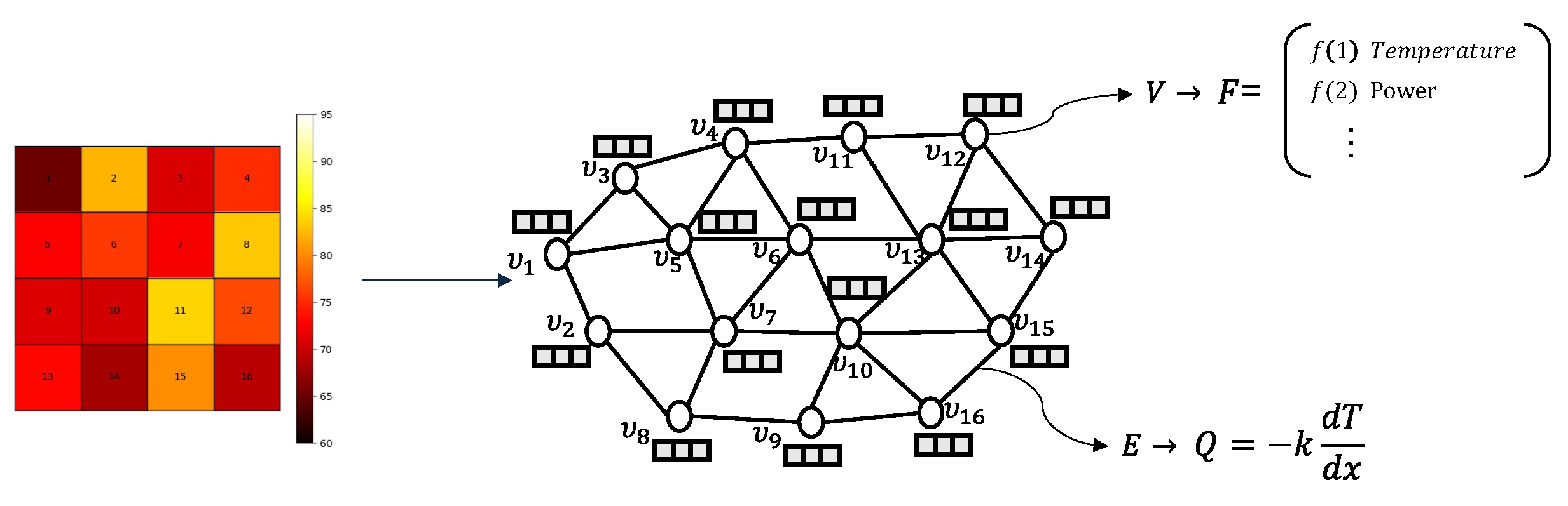
2. Problem Description

Temperature prediction for multi-core chips is crucial to ensuring their performance and reliability. Leveraging the powerful modeling capabilities of GNNs, the complex structure and temperature distribution within the chip can be effectively represented and predicted. We first abstract the thermal system within the chip as a graph $\mathcal{G}=\{\mathcal{V},\mathcal{E}\}$, where the node set $\mathcal{V}=\{v_1,v_2,\cdots v_N\}(N>0)$ represents the heat sources or regions within the chip, and the edge set $\mathcal{E}=\{e_1,e_2,\cdots e_M\}(M>0)$ indicates the thermal transfer relationships between these heat sources. The feature data of the graph $F\in {\mathbb{R}}^{N\times d}$ contains information such as the temperature and power of each node, with d representing the feature dimension, encompassing key parameters like initial temperature and power consumption, as illustrated in Figure 1.

By constructing this graph structure, we can utilize GNNs to capture the complex interplay and information propagation processes between nodes. The node updating mechanism of GNNs allows us to simulate the propagation of heat within the chip, thereby predicting temperature changes in hot spot areas. After training the GNN model, we can learn the thermal conduction patterns between nodes and accurately predict the temperature distribution of hot spots under different operating conditions, thus providing robust data support for chip design and optimization.

3. Methodologies

In this paper, we propose the use of a GCN-based model [28] to address this issue. Additionally, we introduce three methods for constructing the adjacency matrix to suit different application scenarios. First, we employ a graph structure to represent the thermal nodes and their feature data (such as temperature and power) for multi-core chips, building the corresponding adjacency matrix to capture the thermal transfer relationships between nodes. Then, we propose three schemes for constructing the adjacency matrix and perform the necessary preprocessing steps on the feature data to enhance the model’s learning ability for temperature distribution characteristics. Finally, we input the preprocessed data into the convolutional layer of the GCN model and introduce a weighted mechanism for the adjacency matrix. This mechanism allows the adjacency matrix to be updated during the model training process, thereby more accurately capturing the thermal transfer patterns and effectively predicting the temperature distribution of multi-core chips. Through this process, our method not only improves the accuracy of temperature prediction but also enhances the model’s adaptability to the complex thermal dynamics within the chip. Our method is illustrated in Figure 2.

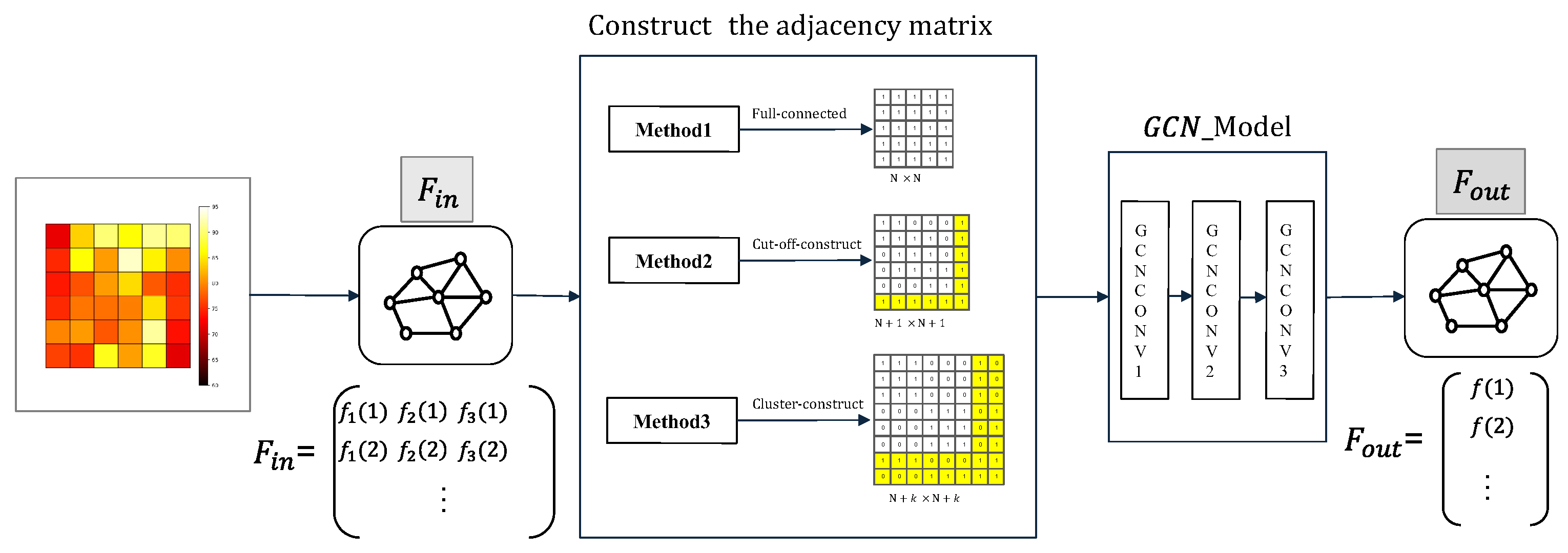
3.1. Model Architecture—GCN-Based Neural Network Model

Our model takes an adjacency matrix along with three key dimensions of features for each thermal node as input: current temperature, historical power, and current power, and outputs the predicted temperature distribution. The structure of the model is shown in Figure 3, which consists of three graph convolutional layers and a fully connected layer.

Additionally, we have employed an improved GCN model that enhances the data training process by introducing learnable edge weights. Compared to traditional GCN models, our approach assigns learnable weight parameters to each edge in the graph. In conventional models, the non-zero elements of the adjacency matrix are typically preset to 1, which means that the graph involved in training is either unweighted or contains fixed weights that are not learnable. This approach limits the model’s ability to capture and learn complex interaction relationships between nodes. The core formula of the traditional GCN is shown as follows:

$$F^{l+1}=\sigma ({\widehat{D}}^{-1/2}A{\widehat{D}}^{-1/2}{F}^l\Theta )$$

(1)

In the formula, $F^l$ represents the node feature matrix and $F^{l+1}$ represents the node feature matrix obtained after a graph convolution operation. A refers to the adjacency matrix that includes self-loops, and D denotes the degree matrix of the nodes. $\Theta$ represents the feature transformation matrix. Considering the impact of the power of the internal core heat sources on the temperature field in the chip, self-loops have been introduced when constructing any adjacency relationships. Based on GCN, we assign learnable weight parameters to each edge, setting the edge weight matrix as E, thus obtaining the following expression:

$$F^{l+1}=\sigma ({\widehat{D}}^{-1/2}\left(A\odot E\right){\widehat{D}}^{-1/2}{F}^l\Theta )$$

(2)

In this context, ⊙ denotes element-wise multiplication and E is a matrix with the same shape and sparsity pattern as A, where each non-zero element represents the weight of each edge in the graph. By assigning learnable weights to the edges, our model can more accurately simulate and learn the information transmission mechanism between nodes, thereby enhancing the network’s performance and prediction accuracy.

3.2. Adjacency Matrix Construction Method

3.2.1. Method 1—Fully Connected Graph

For GNN, we need to design an appropriate adjacency matrix to better represent the temperature transfer relationships between various heat source nodes. We first consider the adjacency matrix $A^{N\times N}$ corresponding to a fully connected graph, as shown in Figure 4.

It can be observed that the fully connected graph structure is dense. Although it captures all the information of the nodes very comprehensively, it also brings several significant issues. In a fully connected graph structure, each node is directly connected to all other nodes, which may include many irrelevant and unimportant connections, losing the structural information of the graph. Overfitting issues may also arise during model training. Moreover, the computation of GCN (Graph Convolutional Network) is mainly related to the number of edges in the graph. The number of edges in a fully connected dense graph is $N^2$, and the computational load increases quadratically with the number of nodes, especially when the graph is large, which undoubtedly greatly increases the computational cost and time. Therefore, the fully connected matrix is suitable for situations with a simple design structure and a small number of heat sources.

3.2.2. Method 2—Setting a Cutoff Radius

To reduce computational complexity, we can design a sparser adjacency matrix. Considering that the temperature between heat source nodes is updated through heat transfer, according to Fourier’s law of heat conduction:

$$Q=-k{\displaystyle \frac{dT}{dx}}$$

(3)

In the equation, Q represents the heat flux density, and it can be observed that Q is directly proportional to the temperature gradient ${\displaystyle \frac{dT}{dx}}$. When considering heat transfer between different hotspots, the distance $dx$ is an important influencing factor. The larger the distance, the smaller the temperature gradient ${\displaystyle \frac{dT}{dx}}$, which in turn leads to a decrease in heat flux density Q. Therefore, the greater the distance between two hotspots, the slower the heat transfer between them, and vice versa. Consequently, we propose setting a cutoff radius $R_0$ based on the Euclidean distance and generating the adjacency matrix according to this cutoff radius, where each node only considers its connections with nearby other nodes. The specific method is as Algorithm 1.

Algorithm 1: Construct Adjacency Matrix with Cutoff Radius Method

1: Input: Coordinate set of N nodes $P=\{(x_1,y_1),(x_2,y_2),\cdots ,(x_N,y_N)\}$ 2: $A\leftarrow \mathrm{Initialize}\mathrm{an}\mathrm{empty}\mathrm{adjacency}\mathrm{matrix}\mathrm{of}\mathrm{size}N\times N$ 3: $R_0\leftarrow$ Set a cutoff radius 4: for  $i\leftarrow 1 \mathrm{to} N$  do 5:    for $j\leftarrow i+1 \mathrm{to} N$ do 6:      $distance\leftarrow \sqrt{{(x_i-x_j)}^2+{(y_i-y_j)}^2}$ 7:      if $distance\le R_0$ then 8:         $A\left[i\right]\left[j\right]\leftarrow 1$ 9:         $A\left[j\right]\left[i\right]\leftarrow 1$ 10:      end if 11:    end for 12: end for 13: return  A

For each node, calculate the Euclidean distance between that node and all other nodes (including itself), and determine whether this distance is less than the cutoff radius $R_0$. If it is less than $R_0$, then establish a connection relationship; otherwise, do not establish a connection relationship. The resulting adjacency matrix is shown in Figure 5 below.

3.2.3. Method 3—Cluster-Based Adjacency Matrix Construction Method

Additionally, we propose another method for constructing the adjacency matrix to optimize the graph structure for internal chip modeling. The method is divided into three steps. First, we set the number of clusters k, and then perform a clustering operation on all nodes to divide them into a fixed number of clusters. Second, for all nodes within each cluster, we establish full connectivity and simultaneously set up a virtual super node for each cluster, which is connected to all the child nodes within its cluster, taking the average of the features of the child nodes as its own. Third, the super nodes of all clusters are fully connected. This method is illustrated in Algorithm 2 and Figure 6.

Algorithm 2 Construct Adjacency Matrix for Clustered Graph

1: Input: $clusters$,k,N 2: $A\leftarrow \mathrm{Initialize}\mathrm{an}\mathrm{empty}\mathrm{adjacency}\mathrm{matrix}\mathrm{of}\mathrm{size}(N+k)\times (N+k)$ 3: for  $cluster \mathrm{in} clusters$  do 4:    $nodes\leftarrow nodes\mathrm{in}cluster$ 5:    for $nodeA,nodeB\mathrm{in}nodes$ do 6:      $A\left[nodeA\right]\left[nodeB\right]\leftarrow 1$ 7:      $A\left[nodeB\right]\left[nodeA\right]\leftarrow 1$ 8:    end for 9:    $superNode\leftarrow \mathrm{virtual}\mathrm{supernode}\mathrm{for}cluster$ 10:    for $node\mathrm{in}nodes$ do 11:      $A\left[superNode\right]\left[node\right]\leftarrow 1$ 12:      $A\left[node\right]\left[superNode\right]\leftarrow 1$ 13:    end for 14: end for 15: for  $superNodeA, superNodeB\mathrm{in}supernodes$  do 16:    $A\left[superNodeA\right]\left[superNodeB\right]\leftarrow 1$ 17:    $A\left[superNodeB\right]\left[superNodeA\right]\leftarrow 1$ 18: end for 19: return  A

It can be seen that, just like the method of setting a cutoff radius, the clustering method is also sensitive to the setting of the number of clusters k. However, considering real application scenarios, setting a cutoff radius may require more parameters or measurement data as a reference, making the selection more complex. On the other hand, we can theoretically calculate a reference value for the number of clusters. Since the computational load of GCNs largely depends on the sparsity of the adjacency matrix, that is, the number of edges, for a graph $\mathcal{G}$ = {$\mathcal{V}$, $\mathcal{E}$}, $\mathcal{V}$ = {$v_1,v_2,\cdots v_N$}, $\mathcal{E}$ = {$e_1,e_2,\cdots e_M$}, we set the number of clusters to k, assuming that the nodes of the entire graph are evenly divided by each cluster, with the number of child nodes in each cluster being n. We can then obtain

$$\left\{\begin{array}{cc}\hfill N& =n\times k\hfill \\ \hfill M& =n^{2}k+k^2\hfill \end{array}\right.$$

Through the above set of equations, we can derive a function for the number of edges M in terms of the number of clusters k:

$$M\left(k\right)={\displaystyle \frac{N^2}{k}}+k^2$$

(4)

By differentiating this function, we can obtain

$$M^{\prime }\left(k\right)=2k-{\displaystyle \frac{N^2}{k^2}}$$

(5)

Setting the above expression to zero, we can find the value of k at which $M\left(k\right)$ takes its minimum value. At this point, $k=\sqrt[3]{{\displaystyle \frac{N^2}{2}}}$. Since k must be an integer, we can take k = $\lfloor k\rfloor$. In this way, we can keep the computational load of the graph to a minimum while more easily determining the value of k. The function is illustrated in Figure 7.

The two methods that we propose can both increase the sparsity of the graph adjacency matrix, thereby reducing computational costs. Different schemes can be selected for different application scenarios under specific circumstances. For example, the method based on the cutoff radius is more sensitive to the setting of the radius size and may perform better when the spatial distribution of hotspots is relatively uniform; whereas the clustering-based method is less sensitive to spatial distribution and easier to determine the number of clusters, which may perform better in situations with irregular spatial distribution.

4. Results

4.1. Dataset Preparation

The dataset used in this paper comes from an open-source simulation tool called MatEx [24]. MatEx is a tool based on matrix exponentials and linear algebra that can quickly and accurately predict the peak temperature of a chip under transient conditions. To perform calculations, MatEx requires users to provide a compact thermal model of the chip, which includes parameters such as the thermal capacitance matrix A, the thermal conductance matrix B, and the ambient temperature vector G, which can typically be obtained through modeling tools like HotSpot. The calculation process of MatEx also requires input files for the spatial layout of the chip’s thermal source cores (including core dimensions and spatial coordinates), as well as power curve files (recording the power values of the thermal source cores at different time points).

We designed layout files containing 16, 36, and 49 nodes, respectively, and assigned random power values between 0 and 20 watts to each thermal core at different time points through a random function to simulate the workload of chip cores under different working conditions. Subsequently, we wrote specialized scripts to work in conjunction with the MatEx tool, thereby generating three datasets containing 5000 sets of data each, as shown in

Table 1. Dataset composition.

Item		Node_Features
Input	Tcurrent	Current core temperature distribution
	Pprevious	Previous core power distribution
	Pcurrent	Current core power distribution
Target	Tnext	Final core temperature distribution
Sample size	5000
Node num	$16\&36\&49$
Train set size	4000
Test set size	1000

in the datasets.

We collected data across three dimensions: current temperature, historical power, and current power, as input features, and used the steady-state temperature distribution data, which can be achieved based on the current power and temperature status obtained from simulation, as label data. We divided the dataset into training and testing sets with a ratio of 4:1.

4.2. Experiments and Results Analysis

4.2.1. Experimental Setup

To effectively evaluate the accuracy of the model proposed in this paper for predicting the internal core temperature distribution of the chip, we respectively adopt MSE and Mean Absolute Error (MAE) as the evaluation metrics for the experiment.

The hardware environment of the experiment is shown in the following

Table 2. Experimental hardware environment.

CPU	Intel(R) Xeon(R) Gold 6230 CPU @ 2.10 GHz (City of Santa Clara, CA, USA)
OS	Ubuntu-20.04
GPU	NVIDIA® V100 Tensor Core (City of Santa Clara, CA, USA)
CUDA-Version	CUDA-11.8

.

The experiment was conducted using Python 3.10.14, and the model construction was based on the PyTorch 1.12.1 framework. The number of training iterations (epochs) was set to 800, the number of samples (batch_size) used to update the weights in each iteration was set to 32, the optimizer used was Adam, and the initial learning rate was set to 0.01. The parameter settings of the experimental model are shown in

Table 3. Experimental parameter settings.

Model layers	Dropout	Train epochs
3	-	800
Batch_size	Learning rate	Learning rate strategy
32	0.01	Cosine Annealing

.

4.2.2. Comparative Experiment of Different Models

To verify the performance of the methods proposed in this paper, we selected the following models and methods, each of which was experimentally compared on datasets with 16, 36, and 49 heat source nodes, respectively:

• MLP: A basic feed-forward neural network composed of multiple fully connected layers, commonly used for classification and regression tasks;
• CNN: CNN is a deep learning architecture that automatically extracts features from images by using convolutional layers and is widely used in image recognition and classification tasks;
• Method 1: Construct an adjacency matrix with all elements set to 1 using a fully connected approach and then train the GCN model;
• Method 2: Construct an adjacency matrix using the cutoff radius method, then train the GCN model;
• Method 3: Construct an adjacency matrix using a clustering method and then train the GCN model.

The experimental results are shown in

Table 4. Comparative experimental results.

Node Num	Model	MSE	MAE
16 Nodes	MLP	1.9	1.07
	CNN	3.11	1.01
	Method 1	0.38	0.51
	Method 2	0.41	0.50
	Method 3	0.43	0.52
36 Nodes	MLP	2.55	1.25
	CNN	2.06	1.45
	Method 1	0.38	0.50
	Method 2	0.41	0.53
	Method 3	0.43	0.50
49 Nodes	MLP	2.65	1.27
	CNN	3.50	1.98
	Method 1	0.38	0.76
	Method 2	0.47	0.55
	Method 3	0.44	0.54

:

4.2.3. Computational Performance Comparative Experiment

• Comparison of Computational and Memory Overheads for Different Methods: The method proposed in this paper aims to achieve real-time prediction of the temperature of multi-core chips. To verify the real-time capability of the model, we analyzed the computational time complexity and memory overhead and evaluated the inference time of different methods. The comparison methods include HotSpot, which is widely used, and MatEx, the chip temperature simulation tool used for generating the dataset in this paper.
  The time complexity and memory overhead of each method are shown in

  Table 5. Analysis of the time complexity and memory overhead of each method.

  Method	HotSpot	MatEx	GCN
  Time complexity	$O\left(N^3\right)$	$O\left(W{N}^2\right)$	$O\left(\right|E\left|f\right)$
  Memory overheads	120 MB	17.45 MB	5.53 MB

  .
  The HotSpot method discretizes the chip structure into N grid nodes. For a 3D structure, the number of grids N increases linearly with the number of layers. However, the overall scale can still be regarded as a polynomial function related to the chip area and the number of layers. The theoretical time complexity is $O\left(N^3\right)$ in the worst-case scenario (when directly solving a dense matrix).
  For the MatEx method, W Newton–Raphson iterations are required for each node. The time complexity of each iteration is $O\left(N\right)$. Therefore, the time complexity for each node is $O\left(WN\right)$, and the total time complexity is $O\left(W{N}^2\right)$.
  For the GCN method, if the adjacency matrix is known a priori, then we only need to consider the time complexity of the multiplication between the feature matrix and the weight matrix, which is approximately $O\left(\right|E\left|f\right)$, where $\left|E\right|$ is the number of edges in the graph, and f is the feature dimension of the nodes. The three adjacency matrix construction strategies that we proposed have different numbers of edges, and the time complexity will vary depending on the specific scenarios and experimental settings.
  In addition, we had each method perform 100 inference predictions for power variations, and the experimental results are shown in Figure 8.
  Our method is at least an order of magnitude faster than the traditional thermal modeling method of HotSpot and the MatEx tool in terms of inference speed. As the number of nodes increases, the difference can reach several orders of magnitude, and the error is small, with the MSE controlled within 0.5. The average time consumption for our model to infer a power change within 2 ms, fully meeting the requirements for real-time temperature prediction;
• Comparison of Different Adjacency Matrices: This paper proposes three strategies for constructing adjacency matrices, each applicable to different scenarios. Therefore, we compared the computational performance of the three strategies. Considering that in GCNs, the most significant factor affecting the time complexity is the number of edges in the graph. We compared the number of edges for the three strategies, as shown in Figure 9.
  From Figure 8, we observe that when the number of nodes is small (i.e., the dimensions of the adjacency matrix are smaller), the sparse matrix does not show an advantage in computational efficiency. Our analysis using the profile tool revealed that, when the number of nodes is small, the access time to matrix data accounts for a larger proportion than the matrix multiplication computation time. Although our proposed Method 3 increases the sparsity, it also increases the dimensions of the adjacency matrix, thus not offering an advantage in low-dimensional matrix access. However, when the number of nodes increases, the computation time becomes a larger proportion than the access time, and the sparsification operations can significantly improve inference efficiency;
• Ablation study of clustering methods: For clustering methods, we have provided a reference method for selecting the number of clusters k, which theoretically can minimize the edges in the adjacency matrix. Therefore, we conducted an ablation study on different numbers of clusters k, while also verifying the number of edges and the model’s predictive accuracy under different conditions. The experimental results are shown in Figure 10.
  It can be observed that, around the reference cluster number k value provided by us, the fluctuation of MSE does not exceed 0.1. Therefore, our method can quickly select the k value, ensuring considerable accuracy while reducing the computational load;
• Power Distribution Sensitivity Experiment: To verify the performance of the model that we designed under different power distributions, we simulated and generated data under various power distributions and then used the model to validate it (49 nodes). It should be noted that we have adopted different random distribution methods for the power of each core, and the power range is between 0 and 20 watts. The results of our experiment are shown in

  Table 6. Analysis of power distribution sensitivity.

  Distribution	Uniform	Gaussian	Exponential
  Accuracy—Method 1 (MSE)	0.38	0.41	0.39
  Accuracy—Method 2 (MSE)	0.47	0.45	0.47
  Accuracy—Method 3 (MSE)	0.44	0.45	0.44

  .
  According to the experiment, our model shows basically consistent performance under different random power distribution methods.

4.2.4. Validation with Real Data

To validate the model’s performance in real-world scenarios, we utilized an open-source real-measurement dataset [29] for performance verification. To ensure the data’s compatibility with our model, we sampled the heatmaps within the data, extracted the node features, and then performed the training process. It is worth clarifying that, given our failure to acquire the floorplan-related data from the dataset, we opted to employ Method 1, as described in the paper for validation.

The experimental results are shown in

Table 7. Experimental results on the real data.

Dataset	Accuracy (MSE)
Google Coral M.2 TPU	0.51
AMD Ryzen 7 4800U	0.73
Intel i5-3337U	0.80

.

As can be seen from the experimental results, our model can still maintain highly accurate temperature prediction in real-world scenarios.

5. Conclusions

This paper proposes a GCN-based framework for real-time temperature prediction in multi-core chips. By mapping thermal nodes and their interdependencies into a graph structure, we introduce three adaptive adjacency matrix construction strategies (full-connection, cutoff radius, and clustering) that balance computational efficiency and accuracy. Experimental results demonstrate that our model achieves a mean squared error (MSE) below 0.5 with inference speeds of 2 ms per prediction—orders of magnitude faster than traditional methods like HotSpot. In addition, we conducted verification on the real-world dataset and achieved a high prediction accuracy.

Future Work Directions: While our method addresses critical gaps in real-time thermal analysis, several promising extensions merit exploration:

• Physics-Informed Hybrid Modeling: Integrating PDE constraints via PINNs could enhance the physical consistency of predictions while retaining GCNs’ computational efficiency. For instance, Fourier’s law of heat conduction could be embedded as a regularization term during training;
• 3D Chiplet Architectures: Extending the graph structure to model vertical heat transfer in stacked-die configurations, where thermal coupling between layers introduces non-uniform conduction patterns;
• Hardware-Software Codesign: Deploying the GCN model on embedded AI accelerators (e.g., NPUs) to achieve sub-millisecond latency for closed-loop thermal management.

References

1. Vaddina, K.R.; Rahmani, A.M.; Latif, K.; Liljeberg, P.; Plosila, J. Thermal modeling and analysis of advanced 3D stacked structures. Procedia Eng. 2012, 30, 248–257. [Google Scholar] [CrossRef]
2. Wang, H.; Tan, S.X.D.; Li, D.; Gupta, A.; Yuan, Y. Composable thermal modeling and simulation for architecture-level thermal designs of multicore microprocessors. ACM Trans. Des. Autom. Electron. Syst. 2013, 18, 1–27. [Google Scholar] [CrossRef]
3. Merrikh, A.A.; McNamara, A.J. Parametric evaluation of foster RC-network for predicting transient evolution of natural convection and radiation around a flat plate. In Proceedings of the Fourteenth Intersociety Conference on Thermal and Thermomechanical Phenomena in Electronic Systems (ITherm), Orlando, FL, USA, 27–30 May 2014; pp. 1011–1018. [Google Scholar] [CrossRef]
4. Jia, W.; Wang, H.; Chen, M.; Lu, D.; Lin, L.; Car, R.; Weinan, E.; Zhang, L. Pushing the Limit of Molecular Dynamics with Ab Initio Accuracy to 100 Million Atoms with Machine Learning. In Proceedings of the SC20: International Conference for High Performance Computing, Networking, Storage and Analysis, Atlanta, GA, USA, 9–19 November 2020; pp. 1–14. [Google Scholar] [CrossRef]
5. Raissi, M.; Perdikaris, P.; Karniadakis, G. Physics-informed neural networks: A deep learning framework for solving forward and inverse problems involving nonlinear partial differential equations. J. Comput. Phys. 2019, 378, 686–707. [Google Scholar] [CrossRef]
6. Ranade, R.; Hill, C.; He, H.; Maleki, A.; Chang, N.; Pathak, J. A composable autoencoder-based iterative algorithm for accelerating numerical simulations. arXiv 2021, arXiv:2110.03780. [Google Scholar]
7. Jin, W.; Sadiqbatcha, S.; Zhang, J.; Tan, S.X.D. Full-Chip Thermal Map Estimation for Commercial Multi-Core CPUs with Generative Adversarial Learning. In Proceedings of the 2020 IEEE/ACM International Conference On Computer Aided Design (ICCAD), Virtual, 2–5 November 2020; pp. 1–9. [Google Scholar]
8. Sadiqbatcha, S.; Zhang, J.; Zhao, H.; Amrouch, H.; Henkel, J.; Tan, S.X.D. Post-Silicon Heat-Source Identification and Machine-Learning-Based Thermal Modeling Using Infrared Thermal Imaging. IEEE Trans. Comput.-Aided Des. Integr. Circuits Syst. 2021, 40, 694–707. [Google Scholar] [CrossRef]
9. Chen, L.; Jin, W.; Tan, S.X.D. Fast Thermal Analysis for Chiplet Design based on Graph Convolution Networks. In Proceedings of the 2022 27th Asia and South Pacific Design Automation Conference (ASP-DAC), Taipei, Taiwan, 17–20 January 2022; pp. 485–492. [Google Scholar] [CrossRef]
10. Bhatasana, M.; Marconnet, A. Deep Learning for Real-Time Chip Temperature and Power Predictions. In Proceedings of the 2023 22nd IEEE Intersociety Conference on Thermal and Thermomechanical Phenomena in Electronic Systems (ITherm), Orlando, FL, USA, 30 May–2 June 2023; pp. 1–7. [Google Scholar] [CrossRef]
11. Grailoo, M.; Nunez-Yanez, J. Heterogeneous Edge Computing for Molecular Property Prediction with Graph Convolutional Networks. Electronics 2025, 14, 101. [Google Scholar] [CrossRef]
12. Ye, Z.; Wang, H.; Przystupa, K.; Majewski, J.; Hots, N.; Su, J. Dynamic Spatio-Temporal Hypergraph Convolutional Network for Traffic Flow Forecasting. Electronics 2024, 13, 4435. [Google Scholar] [CrossRef]
13. Guggari, S.I. Analysis of Thermal Performance Metrics—Application to CPU Cooling in HPC Servers. IEEE Trans. Compon. Packag. Manuf. Technol. 2021, 11, 222–232. [Google Scholar] [CrossRef]
14. Heinig, A.; Fischbach, R.; Dittrich, M. Thermal analysis and optimization of 2.5D and 3D integrated systems with Wide I/O memory. In Proceedings of the Fourteenth Intersociety Conference on Thermal and Thermomechanical Phenomena in Electronic Systems (ITherm), Orlando, FL, USA, 27–30 May 2014; pp. 86–91. [Google Scholar] [CrossRef]
15. Zhou, J.; Yan, J.; Cao, K.; Tan, Y.; Wei, T.; Chen, M.; Zhang, G.; Chen, X.; Hu, S. Thermal-aware correlated two-level scheduling of real-time tasks with reduced processor energy on heterogeneous MPSoCs. J. Syst. Archit. 2018, 82, 1–11. [Google Scholar] [CrossRef]
16. Bogdan, P.; Marculescu, R.; Jain, S. Dynamic power management for multidomain system-on-chip platforms: An optimal control approach. ACM Trans. Des. Autom. Electron. Syst. 2013, 18, 1–20. [Google Scholar] [CrossRef]
17. Kim, Y.G.; Kim, M.; Kong, J.; Chung, S.W. An Adaptive Thermal Management Framework for Heterogeneous Multi-Core Processors. IEEE Trans. Comput. 2020, 69, 894–906. [Google Scholar] [CrossRef]
18. Zhang, J.; Sadiqbatcha, S.; Tan, S.X.D. Hot-Trim: Thermal and Reliability Management for Commercial Multicore Processors Considering Workload Dependent Hot Spots. IEEE Trans. Comput.-Aided Des. Integr. Circuits Syst. 2023, 42, 2290–2302. [Google Scholar] [CrossRef]
19. Lin, J.Y.; Lin, S.Y. Temperature-Prediction Based Rate-Adjusted Time and Space Mapping Algorithm for 3D CNN Accelerator Systems. IEEE Trans. Comput. 2023, 72, 2767–2780. [Google Scholar] [CrossRef]
20. Huang, W.; Ghosh, S.; Velusamy, S.; Sankaranarayanan, K.; Skadron, K.; Stan, M. HotSpot: A compact thermal modeling methodology for early-stage VLSI design. IEEE Trans. Very Large Scale Integr. (VLSI) Syst. 2006, 14, 501–513. [Google Scholar] [CrossRef]
21. Chen, T.Y.; Kuo, S.L.; Hsu, J.M.; Pan, C.W. Dynamic compact thermal modeling of package-on-package by thermal resistor-capacitor ladder. In Proceedings of the 2016 15th IEEE Intersociety Conference on Thermal and Thermomechanical Phenomena in Electronic Systems (ITherm), Las Vegas, NV, USA, 31 May–3 June 2016; pp. 223–229. [Google Scholar] [CrossRef]
22. Jiang, L.; Dowling, A.; Liu, Y.; Cheng, M.C. Chip-level Thermal Simulation for a Multicore Processor Using a Multi-Block Model Enabled by Proper Orthogonal Decomposition. In Proceedings of the 2022 21st IEEE Intersociety Conference on Thermal and Thermomechanical Phenomena in Electronic Systems (iTherm), San Diego, CA, USA, 31 May–3 June 2022; pp. 1–7. [Google Scholar] [CrossRef]
23. Jiang, L.; Dowling, A.; Cheng, M.C.; Liu, Y. PODTherm-GP: A Physics-Based Data-Driven Approach for Effective Architecture-Level Thermal Simulation of Multi-Core CPUs. IEEE Trans. Comput. 2023, 72, 2951–2962. [Google Scholar] [CrossRef]
24. Pagani, S.; Chen, J.J.; Shafique, M.; Henkel, J. MatEx: Efficient transient and peak temperature computation for compact thermal models. In Proceedings of the 2015 Design, Automation & Test in Europe Conference & Exhibition (DATE), Grenoble, France, 9–13 March 2015; pp. 1515–1520. [Google Scholar] [CrossRef]
25. Juan, D.C.; Zhou, H.; Marculescu, D.; Li, X. A learning-based autoregressive model for fast transient thermal analysis of chip-multiprocessors. In Proceedings of the 17th Asia and South Pacific Design Automation Conference, Sydney, NSW, Australia, 30 January–2 February 2012; pp. 597–602. [Google Scholar] [CrossRef]
26. Zhang, K.; Guliani, A.; Ogrenci-Memik, S.; Memik, G.; Yoshii, K.; Sankaran, R.; Beckman, P. Machine Learning-Based Temperature Prediction for Runtime Thermal Management Across System Components. IEEE Trans. Parallel Distrib. Syst. 2018, 29, 405–419. [Google Scholar] [CrossRef]
27. Ranade, R.; He, H.; Pathak, J.; Chang, N.; Kumar, A.; Wen, J. A Thermal Machine Learning Solver For Chip Simulation. In Proceedings of the 2022 ACM/IEEE 4th Workshop on Machine Learning for CAD (MLCAD), Snowbird, UT, USA, 12–13 September 2022; pp. 111–117. [Google Scholar] [CrossRef]
28. Kipf, T.; Welling, M. Semi-Supervised Classification with Graph Convolutional Networks. arXiv 2016, arXiv:1609.02907. [Google Scholar]
29. Lu, J.; Tan, S.X.D. Thermal Map Dataset for Commercial Multi/Many Core CPU/GPU/TPU. In Proceedings of the 2024 ACM/IEEE International Symposium on Machine Learning for CAD, Salt Lake City, UT, USA, 9–11 September 2024. [Google Scholar] [CrossRef]
Figure 1. Chip graph structure thermal model.
Electronics 14 01223 g001
Figure 2. Method framework.
Electronics 14 01223 g002
Figure 3. GCN network model.
Electronics 14 01223 g003
Figure 4. Fully connected graph G that includes self-loops.
Electronics 14 01223 g004
Figure 5. Graph G with self-loops generated by setting a cutoff radius.
Electronics 14 01223 g005
Figure 6. Cluster-based method constructed graph G .
Electronics 14 01223 g006
Figure 7. Schematic diagram of the function M ( k ) (when N = 36).
Electronics 14 01223 g007
Figure 8. Comparison of inference times for different methods.
Electronics 14 01223 g008
Figure 9. The number of edges in the graph for different methods.
Electronics 14 01223 g009
Figure 10. The number of edges and predictive accuracy (MSE) for different numbers of nodes (a) 16 nodes, (b) 36 nodes, (c) 49 nodes.
Electronics 14 01223 g010