Abstract
Scene understanding is essential for enhancing driver safety, generating human-centric explanations for Automated Vehicle (AV) decisions, and leveraging Artificial Intelligence (AI) for retrospective driving video analysis. This study developed a dynamic scene retrieval system using Contrastive Language–Image Pretraining (CLIP) models, which can be optimized for real-time deployment on edge devices. The proposed system outperforms state-of-the-art in-context learning methods, including the zero-shot capabilities of GPT-4o, particularly in complex scenarios. By conducting frame-level analyses on the Honda Scenes Dataset, which contains a collection of about 80 h of annotated driving videos capturing diverse real-world road and weather conditions, our study highlights the robustness of CLIP models in learning visual concepts from natural language supervision. The results also showed that fine-tuning the CLIP models, such as ViT-L/14 (Vision Transformer) and ViT-B/32, significantly improved scene classification, achieving a top F1-score of 91.1%. These results demonstrate the ability of the system to deliver rapid and precise scene recognition, which can be used to meet the critical requirements of advanced driver assistance systems (ADASs). This study shows the potential of CLIP models to provide scalable and efficient frameworks for dynamic scene understanding and classification. Furthermore, this work lays the groundwork for advanced autonomous vehicle technologies by fostering a deeper understanding of driver behavior, road conditions, and safety-critical scenarios, marking a significant step toward smarter, safer, and more context-aware autonomous driving systems.
1. Introduction
Understanding scenes is considered one of the most challenging tasks for improving driver safety and enhancing the performance of advanced driver assistance systems (ADASs) [1,2]. The use of AI in this field has opened new dimensions for the retrospective analysis of driving videos. This enables the analysis of driver behavior in terms of gap identification in driving skills and assessment of overall driving performance [3,4,5]. The role of AI in improving scene understanding is further emphasized by its ability to process massive volumes of driving data. For example, machine learning techniques, like Long Short-Term Memory (LSTM) networks, have been applied to classify and predict driver behavior based on real-time data [6].
It will have the possibility to develop systems able to not only learn a particular style of driving but also to adapt themselves to environmental conditions to optimize safety performance. Additionally, AI in ADASs means continuous monitoring of driver behavior, whereby at any given moment the system could give some feedback or even intervene [7]. AI significantly increases vehicular situational awareness and, subsequently, decision-making processes by processing and analyzing data from a wide range of sensors, such as cameras and LiDAR [8]. Furthermore, driver acceptance of ADAS can be better understood by gaining insights into how drivers will respond to automated systems, especially in terms of reliance and trust [9]. The extent to which the drivers may be willing to utilize these systems can be greatly impacted by the driver’s perception of the systems reliability [10,11].
Hence, it is vital to devise and build an ADAS that can support drivers and produce synergy between humans and machines. This necessity brings a spotlight to systems that can understand and react to the ever-changing landscape of driving to improve the overall safety and efficiency of driving. Driver training and understanding of these technologies are other important factors that also affect the working of the ADAS. The evidence suggests that training can impact drivers’ knowledge regarding the capabilities and limitations of ADASs and, consequently, acceptance and trust in automation [12]. This is specifically relevant because motorists rely more and more on these systems for safety and assistance. For driver mental models, the design of the ADAS must, therefore, take into account not only the technological capacities of the drivers but also their mental models and interaction with the systems in question [13]. This ability of AI to perceive the scene has been extended by its ability to scan millions of driving hours of data.
This study presents a new framework for dynamic scene understanding enabled by the Contrastive Language–Image Pretraining (CLIP) model. The key contributions of this work are as follows: (1) We propose a CLIP-based retrieval system for real-time decision-making in an ADAS and demonstrate its effectiveness in understanding dynamic driving scenes, which can be used for real-time deployment on edge devices. (2) We benchmarked the performance of the CLIP model against state-of-the-art in-context learning methods, including the zero-shot capabilities of GPT-4o, highlighting the superior performance of CLIP for scene classification. (3) We apply a frame-level analysis of the publicly available Honda Scenes Dataset, incorporating diverse road and environmental conditions to enable the robust classification of traffic scenes. (4) This study then shows how multimodal AI can add depth to the recognition of road conditions and driver behavior to provide meaningful insights into autonomous driving systems and road safety research. Thus, this study lays the foundation for further research on the effective integration of language-based supervision with visual scene recognition within ADAS applications.
This study does not introduce a new deep learning model but rather optimizes and benchmarks existing CLIP architectures for real-time scene classification in autonomous driving. By integrating CLIP with a high-performance retrieval system and conducting extensive fine-tuning, we demonstrate significant improvements in accuracy and efficiency over state-of-the-art in-context learning models, such as GPT-4o. Our contributions lie in adapting CLIP models to real-time ADAS applications, evaluating their scalability on automotive-grade hardware, and providing a robust framework for multimodal scene understanding.
The rest of the paper is organized as follows: Section 2 describes the literature review on current approaches and advancements in the field of scene understanding and ADAS technologies. Section 3 provides a background and comparison between the CLIP models used in this study. Section 4 outlines the methodology, detailing how the proposed CLIP-based retrieval system was implemented. Section 5 discusses the dataset and preprocessing, focusing on the Honda Scenes Dataset and how it was prepared for analysis. The results can be found in Section 6, where the system performance is compared with the state-of-the-art methods. Section 7 discusses the findings and their implications. Finally, the conclusions are drawn in Section 8, summarizing the paper’s contributions toward advances in multimodal AI for dynamic scene understanding.
2. Literature Review
Scene understanding is very significant in transportation, furthered by the need for the interaction of a vehicle with the road and its surroundings [14,15]. In relation, the work by Pham et al. regarding joint geometric and object segmentation stipulates the significance of proper identification and classification of objects within indoor scenes into the settings of transportation [16]. The improvement in accuracy while detecting objects helps vehicles to make better interpretations and subsequent decisions.
These basic methods are all about the employment of Convolutional Neural Networks (CNNs) for scene analysis and classification according to their semantic contents. CNNs are pretty good at extracting features from images, thus providing a way of identifying objects and their relations within a scene. For example, Li et al. have indicated that deep learning approaches have dominated the evolution of scene understanding, especially with CNNs that outperform the traditional approaches, such as K-means and SVMs (Support Vector Machines) [17]. Ni et al. gave more weight to this claim when they proposed a deep network-based improved method of scene classification specifically designed for a self-driving car, enhanced by a novel Inception module in both global and local feature extraction [18]. The robustness and accuracy of feature fusion tremendously upgrade the performance of scene classification for the safe driving of an ego vehicle in a complex real environment.
Guo et al. (2021) [19] provided a comprehensive survey of deep learning-based approaches for scene understanding in autonomous driving, categorizing research into object detection, semantic segmentation, instance segmentation, and lane line segmentation. While CNNs have been instrumental in feature extraction and object recognition, they often face challenges in capturing long-range dependencies and contextual information within a scene. This limitation has prompted exploration into more advanced architectures that can better model global contexts [19].
The Vision Transformer (ViT) model, introduced by Dosovitskiy et al. (2020) [20], represents a paradigm shift by employing a transformer-based architecture for image recognition tasks. ViT divides images into patches and processes them similarly to words in natural language processing, effectively capturing global relationships. However, ViT models require substantial computational resources and large-scale datasets for effective training, which can be a barrier to their deployment in real-time systems.
In the realm of multimodal learning, the Contrastive Language–Image Pretraining (CLIP) model, developed by Radford et al. (2021) [21], has demonstrated remarkable zero-shot transfer capabilities across various domains. CLIP learns visual concepts from natural language supervision, enabling it to perform a wide range of tasks without task-specific fine-tuning. Despite its versatility, the application of CLIP in autonomous driving is still emerging, with challenges related to real-time performance and integration with existing perception systems.
Guo et al. (2023) [14] explore the use of multi-task learning to enhance road scene understanding for autonomous vehicles. Their approach aims to develop a perception model that balances size, speed, and accuracy, addressing the need for efficient processing in resource-constrained environments. While their model shows promise, its performance can be affected by varying lighting and weather conditions, indicating the necessity for robust adaptation mechanisms [14].
Complementary to CNNs, the integration of methods for 3D scene understanding will play an increasingly important role in tasks such as autonomous vehicles. The model proposed by Han et al. predicts a 3D scene graph that describes entities within a scene and gives semantic relationships among these entities for enhanced environmental understanding [22]. This approach bridges an important gap in the literature on scene understanding because traditional methods are usually insensitive to the relations between objects. Moreover, LiDAR combined with deep learning has been demonstrating encouraging results on the estimation of scene flow and relative pose, which was introduced by Li et al. in the study of LiDAR odometry for unmanned ground vehicles [23]. Taken together, these technologies enable real-time processing and, therefore, precise mapping in dynamic environments, which is very important for good navigation.
Another challenge was the proper detection and classification of various road conditions, from potholes to wet surfaces, through novel machine learning. Vernekar et al. developed another type of pipeline using pretrained models to analyze live images captured from traffic cameras. This refines the existing feature extraction process to enhance the accuracy in detection [24]. This approach not only enhances the reliability of understanding scenes but also contributes significantly to the safety of transportation systems by enabling timely responses to hazardous situations.
The use of synthetic data generation to train AI models is increasing in the field of scene understanding. Holst et al. talk about generating synthetic training data for robotics applications, which can be adapted for various transportation scenarios [25]. Using simulations of diverse environments and conditions, researchers can create robust datasets that improve the performance of machine learning models in real-world applications.
Another critical aspect of scene understanding related to transportation is the integration of multimodal data sources. For instance, the work of Zipfl and Zöllner insists that image-based approaches must combine with graph-based methods representing spatial environmental factors and their relations regarding traffic participants [26].
This paper presents a new framework of dynamic understanding based on the CLIP model. The main contributions of this work are as follows: (1) A CLIP-based retrieval system for real-time decision-making in ADAS applications is proposed and demonstrates its effectiveness in understanding dynamic driving scenes. (2) CLIP performance is compared to the state-of-the-art in-context learning methods, including zero-shot performance for GPT-4o. This is to show that CLIP performs best on the task of scene classification. (3) A frame-level analysis is performed on the publicly available Honda Scenes Dataset, which includes a wide variety of road and environmental conditions that can enable robust traffic scene classification. (4) The work investigates how to effectively integrate language-based supervision with visual scene recognition, providing meaningful insights into road safety research and autonomous driving systems by laying the bedrock for further advancements in multimodal AI.
3. Contrastive Language–Image Pretraining (CLIP)
CLIP models have significantly advanced the field of vision-language understanding by learning visual representations from natural language supervision [21]. One advantage of using CLIP is that it can be deployed on edge devices with careful consideration of hardware capabilities, model size, and optimization techniques. While smaller variants (e.g., ViT-B/32) are more practical for edge use, larger variants, like ViT-L/14, may require significant optimizations or hybrid deployment strategies. ViT (Vision Transformer) models differ in size and complexity. “B” (Base) and “L” (Large) indicate model depth, while the number (e.g., 32 in ViT-B/32) represents the image patch size. Smaller patch sizes (e.g., 14 in ViT-L/14) capture more detail but require more computation. The choice ultimately depends on the application’s real-time requirements, available resources, and the complexity of the scene understanding tasks. Various CLIP model architectures have been developed, each with distinct characteristics concerning model size, processing speed, VRAM requirements, and architectural design. This document compares five prominent CLIP models—ViT-B/32, ViT-B/16, ViT-L/14, RN50, and RN101—in terms of their number of parameters, processing speed, VRAM requirements for embedding, and architectural differences. We selected these five CLIP models (ViT-B/32, ViT-B/16, ViT-L/14, RN50, and RN101) to cover a range of trade-offs between accuracy, computational cost, and deployment feasibility. The ViT models provide strong global feature extraction, with ViT-L/14 offering the highest accuracy but requiring more resources. Meanwhile, ResNet-based models (RN50, RN101) are included for their efficient convolutional processing, which can be advantageous for real-time applications. This selection allows us to compare different architectures and assess their suitability for autonomous driving tasks. The goal is to provide insights into their suitability for different applications, aiding in the selection of an appropriate model based on specific requirements. The following is a comparison between the different CLIP models.
3.1. Number of Parameters
The number of parameters in a model is a crucial factor influencing its computational requirements and potential performance. Models with more parameters can capture more complex patterns but require more computational resources for training and inference. Table 1 summarizes the number of parameters for each CLIP model under consideration. The text encoder parameters are consistent across models, except for ViT-L/14, which uses a larger text encoder.

Table 1.
Number of parameters in CLIP models.
3.2. Processing Speed (Frames per Second)
Processing speed is a critical factor, especially for real-time applications. It depends on the model’s complexity, computational requirements, and the hardware used. Table 2 provides approximate frames per second (FPS) for each model on a high-end GPU (e.g., NVIDIA RTX 3090). It is worth noting that these are rough estimates. The actual performance may vary based on hardware specifications, software optimizations, and batch size.
Table 2.
Approximate processing speed of CLIP models.
3.3. Models Architecture
The architecture of a model influences its ability to capture features, computational efficiency, and suitability for different tasks. The CLIP models considered here are based on two primary architectures: Vision Transformers (ViT) and ResNets.
Vision Transformers apply transformer architectures to sequences of image patches, leveraging self-attention mechanisms to model global relationships within an image [20]. Key architectural details of the ViT-based CLIP models are provided in Table 3. Note that the number of patches is calculated by dividing the image dimensions by the patch size and squaring the result.
Table 3.
Architectural details of ViT-based CLIP models.
ResNet models utilize convolutional neural networks (CNNs) with residual connections, enabling the training of deeper networks by mitigating the vanishing gradient problem [27]. ResNet-based CLIP models, such as RN50 and RN101, use convolutional neural networks (CNNs) with residual connections, allowing for deep feature extraction while mitigating vanishing gradient issues. Unlike ViT models, which process images as sequences of patches using self-attention, ResNet models apply hierarchical feature extraction through convolutional layers. This makes ResNet-based models generally faster for inference but less effective at capturing global contextual relationships compared to ViT models. Architectural details of the ResNet-based CLIP models are provided in Table 4.
Table 4.
Architectural details of ResNet-based CLIP models.
However, ViT models process images as sequences of patches and rely on self-attention mechanisms to capture global context. In contrast, ResNet models use convolutional layers to capture local spatial hierarchies and employ residual connections to facilitate the training of deep networks. Moreover, ViT-L/14 is significantly larger than the ViT-B models and ResNet models due to more layers and a larger hidden size. It is also worth noting that smaller patch sizes in ViT models (e.g., ViT-B/16 and ViT-L/14) result in more patches per image, allowing the model to capture finer details but increasing the computational load.
3.4. VRAM Requirements for Embedding
The amount of VRAM (Video Random Access Memory) required for embedding using each model is a crucial consideration, especially when deploying models on GPUs with limited memory. VRAM requirements can vary based on factors such as batch size and implementation details. Approximate requirements for inference with a batch size of 1 are provided in Table 5. Note that VRAM requirements increase with larger batch sizes and higher-resolution images.
Table 5.
Approximate VRAM requirements for embedding.
Table 5 showed that CLIP ViT-B/32 requires the least VRAM among ViT models, making it suitable for devices with limited GPU memory. It also showed that CLIP ViT-L/14 has the highest VRAM requirement due to its large number of parameters and deeper architecture. Nonetheless, ResNet models generally have moderate VRAM requirements, with RN101 requiring more memory than RN50 due to its deeper architecture.
Other considerations include that models with higher VRAM requirements may not be suitable for deployment on devices with limited GPU memory. Selecting a model involves balancing the need for speed, accuracy, and memory consumption, and increasing the batch size will proportionally increase the VRAM usage. The careful management of batch sizes is necessary to avoid memory overflow.
3.5. Summary and Recommendations
Table 6 shows the pros, cons, and recommendations for the different CLIP models. To select a model between them, it is important to consider several factors. The first one is resource availability, which includes ensuring that computational resources (e.g., GPU memory, processing power) are sufficient for the chosen model, especially for larger models, like ViT-L/14, and assessing VRAM availability to prevent out-of-memory errors during embedding. The second one is application requirements, in which determining whether speed, accuracy, or memory efficiency is the priority and understanding that real-time applications may benefit from faster models with lower VRAM requirements, like ViT-B/32 or RN50. Finally, model familiarity, in which it is recommended to select a model architecture that aligns with the development team’s expertise, while understanding that ResNet models may be preferable for those more familiar with convolutional neural networks and ViT models may offer advantages in tasks where capturing global context is important.
Table 6.
Pros, cons, and recommendations for different CLIP models.
Nonetheless, selecting the appropriate CLIP model involves balancing the application’s performance requirements with the available computational resources, including VRAM. CLIP ViT-B/32 and CLIP RN50 are recommended for applications prioritizing speed and memory efficiency. CLIP ViT-B/16 and CLIP RN101 offer a middle ground between performance, resource demands, and VRAM usage. For tasks where maximum accuracy and detail are critical, CLIP ViT-L/14 is ideal, provided that sufficient computational resources and GPU memory are available.
Automotive-grade GPUs play a crucial role in enabling real-time AI processing for ADASs and autonomous vehicles. Platforms such as NVIDIA DRIVE AGX Orin (275 TOPS), Intel Arc A760A (14 TFLOPS FP32), and AMD Radeon RX 6000 Series provide scalable solutions for in-vehicle AI workloads. The choice of GPU directly impacts the feasibility of deploying CLIP models in real-world driving scenarios, where balancing computational efficiency with model accuracy is critical. Future research should explore optimized implementations tailored for automotive hardware constraints.
4. Proposed Methodology
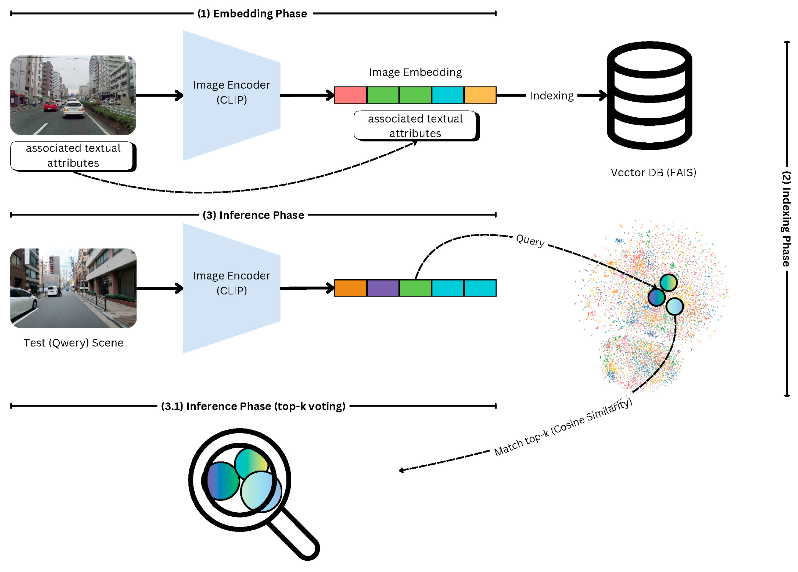
Our methodology aims to establish a real-time scene understanding framework that serves as a critical component for advanced driver assistance systems. These systems necessitate rapid and accurate comprehension of driving environments to provide drivers with timely, context-aware advice. Our framework is built on two key pillars, namely, embedding scene images and efficient indexing. Figure 1 provides a high-level overview of the proposed methodology. In the following subsections, we will present a detailed explanation of each component.

Figure 1.
A high-level overview of the proposed scene understanding methodology, integrating CLIP-based embeddings, FAISS indexing, and similarity-based retrieval for efficient scene understanding.
4.1. Embedding Scene Images with CLIP
We leverage the Contrastive Language–Image Pretraining (CLIP) model to embed scene images into a high-dimensional vector space. CLIP is a robust model known for its ability to associate textual descriptions with visual data effectively. It captures semantic relationships between visual elements and their corresponding textual attributes, transforming complex visual scenes into embeddings suitable for computational processing. These embeddings allow our framework to map driving scenes into a representation that preserves the underlying semantic structure, making it ideal for real-time retrieval and analysis.
In this study, we fine-tuned the CLIP ViT-B/32 and CLIP ViT-L/14 models on the Honda Scenes Dataset. The fine-tuning process involved optimizing the models with a dataset-specific retrieval objective, where scene images were paired with natural language descriptions representing their attributes (e.g., “urban intersection with pedestrian crossing”). The objective was to enhance CLIP’s ability to distinguish fine-grained traffic scenarios while maintaining efficient inference times for real-time applications.
4.2. Efficient Indexing with FAISS (Facebook AI Similarity Search)
Since autonomous driving requires real-time scene classification, traditional deep learning-based retrieval methods can be computationally expensive. To ensure efficient retrieval and reduce latency, we integrated FAISS, a high-performance similarity search library, for indexing and searching scene embeddings. FAISS allows the model to quickly identify the most relevant past driving scenarios based on query embeddings, ensuring rapid and accurate decision-making.
To manage and search through the high-dimensional embeddings generated by CLIP, we incorporate the Facebook AI Similarity Search (FAISS). FAISS is an advanced library optimized for similarity search and clustering of dense vectors. Known for its scalability and speed, FAISS is designed to handle large datasets with high-dimensional data efficiently. By utilizing FAISS, we index the CLIP-generated embeddings, enabling the rapid retrieval of the most relevant scenes. This integration is crucial for real-time applications where speed and precision are essential, as FAISS supports approximate nearest neighbor search, ensuring quick access to relevant information even in large-scale scenarios.
The integration of CLIP and FAISS creates a powerful real-time scene understanding framework. CLIP converts visual data into a searchable vector space, while FAISS ensures that the retrieval process is both swift and accurate. Together, they provide the computational backbone for processing and interpreting driving scenes promptly, empowering the system to deliver timely and precise advice to drivers, enhancing safety and decision-making.
4.3. Inference Phase
During the inference phase, the framework processes a test scene through the CLIP model to generate its embedding. This embedding is then queried in the FAISS index to identify the nearest neighbor scenes. The textual attributes associated with these nearest neighbors are retrieved, and for each attribute, the system predicts the value based on the majority vote among the retrieved neighbors. This process ensures that the predictions are both data-driven and contextually relevant.
The inference phase consists of the following steps:
- Scene Embedding Generation, where the input scene image is passed through the fine-tuned CLIP model to obtain a feature vector in the latent space.
- Similarity Search via FAISS, where the generated embedding is compared against a pre-indexed FAISS database to retrieve the most relevant past driving scenarios.
- Scene Classification and Labeling, where based on the retrieved nearest neighbors, the system assigns a label to the current scene using a majority voting mechanism.
- Decision Support for ADAS, where the retrieved contextual information is used to enhance situational awareness in the ADAS system, improving autonomous decision-making.
4.4. Models Fine-Tuning
Following the evaluation, the top-performing CLIP models are selected for fine-tuning. Fine-tuning aligns the embedding space more closely with the semantic requirements of scene understanding, allowing the model to capture subtle nuances in driving contexts. The fine-tuned models are then used to embed the training data into a newly refined vector space. A new FAISS index is built using these embeddings, enabling the retrieval of nearest neighbors for test scenes that have been embedded using the fine-tuned models. This alignment significantly improves the model’s ability to predict scene attributes with greater precision and recall. The combination of CLIP and FAISS not only ensures real-time performance but also provides a flexible framework that can adapt to new scenarios through fine-tuning. By aligning the embedding space to the semantics of scene understanding, the methodology enhances the accuracy and robustness of predictions.
To address the limitation of the CLIP model’s text encoder, which imposes a 77-token restriction, we implemented an efficient text description generation approach using the following method. This method encodes textual descriptions by coding attribute values using numbers and then converting them into a concise string, joining them in a predefined order with commas to ensure the text remains compact and within the token limit. By focusing solely on the attribute values, the encoded descriptions effectively preserve the semantic relationships between similar images, ensuring that they are clustered closely in the latent space. Meanwhile, the detailed textual descriptions of the attributes are stored separately in a file and indexed for retrieval through FAISS. This dual approach guarantees computational efficiency while maintaining the richness of the original attribute descriptions for downstream tasks.
5. Dataset Description
The Honda Scenes Dataset (HSD) is a large-scale annotated dataset designed to support dynamic traffic scene classification. Comprising 80 h of high-quality driving video data collected from the San Francisco Bay Area, HSD offers a rich variety of scenarios for training and testing. The dataset includes 11 road place classes, such as three-way intersections, four-way intersections, zebra crossings, and construction zones. It also spans four road environments (rural, urban, highway, and ramp) and four weather conditions (rainy, sunny, cloudy, and foggy). Detailed annotations are available in the JSON and CSV formats, capturing temporal and frame-level attributes like road conditions, surface conditions, and event sub-classes such as “approaching”, “entering”, and “passing”. Specialized sub-classes for merges and branches allow for a granular analysis, enhancing the dataset’s utility in various traffic-related research contexts.
The preprocessing methodology involves systematic steps to prepare the data for analysis, as shown in Figure 2. The dataset is pre-split into training and testing sets to ensure no spatial overlap between trips, maintaining the independence of the test data for a robust evaluation. The training data are outlined in trainsplit.txt, while the testing data are defined in valsplit.txt. The videos are converted into individual frames to facilitate the frame-level analysis. The frames in the test set are downsampled to one frame per second, while those in the training set are downsampled to one frame every two seconds, reducing the computational demands while retaining essential information. Frames with all 21 attributes set to zero are filtered out, ensuring that only frames with meaningful annotations are included in the analysis. This preprocessing approach supports the efficient and effective use of the dataset for training and evaluation purposes.
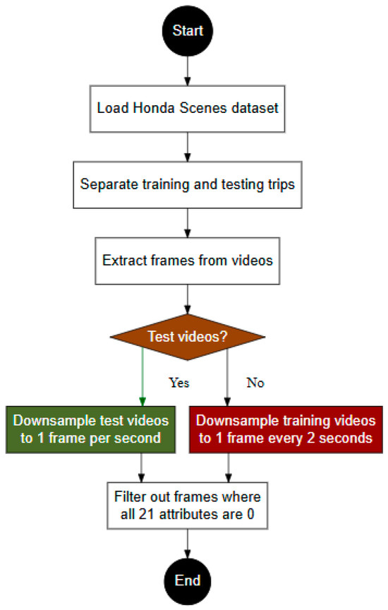
Figure 2.
Overview of the data preprocessing workflow: steps include splitting the Honda Scenes Dataset into training and testing, extracting frames from videos, downsampling at different rates for training and testing, and filtering out frames with no relevant information.
Our experiments are conducted on the Honda Scenes Dataset, which provides a diverse range of driving scenarios, including variations in weather conditions, road lighting, and environmental complexities. This dataset is specifically designed for scene understanding in autonomous driving applications, making it a suitable benchmark for evaluating our proposed models. To the best of our knowledge, no other publicly available dataset offers a comparable level of detail for this specific task. While we acknowledge the importance of evaluating our approach on additional datasets, current limitations in publicly accessible alternatives prevent us from doing so. Additionally, the creation of a new dataset requires significant financial and logistical resources, which are beyond the scope of this study. However, we are actively exploring potential datasets for future evaluations to further validate our findings and ensure broader generalizability.
6. Experimental Work
6.1. Prompt Engineering
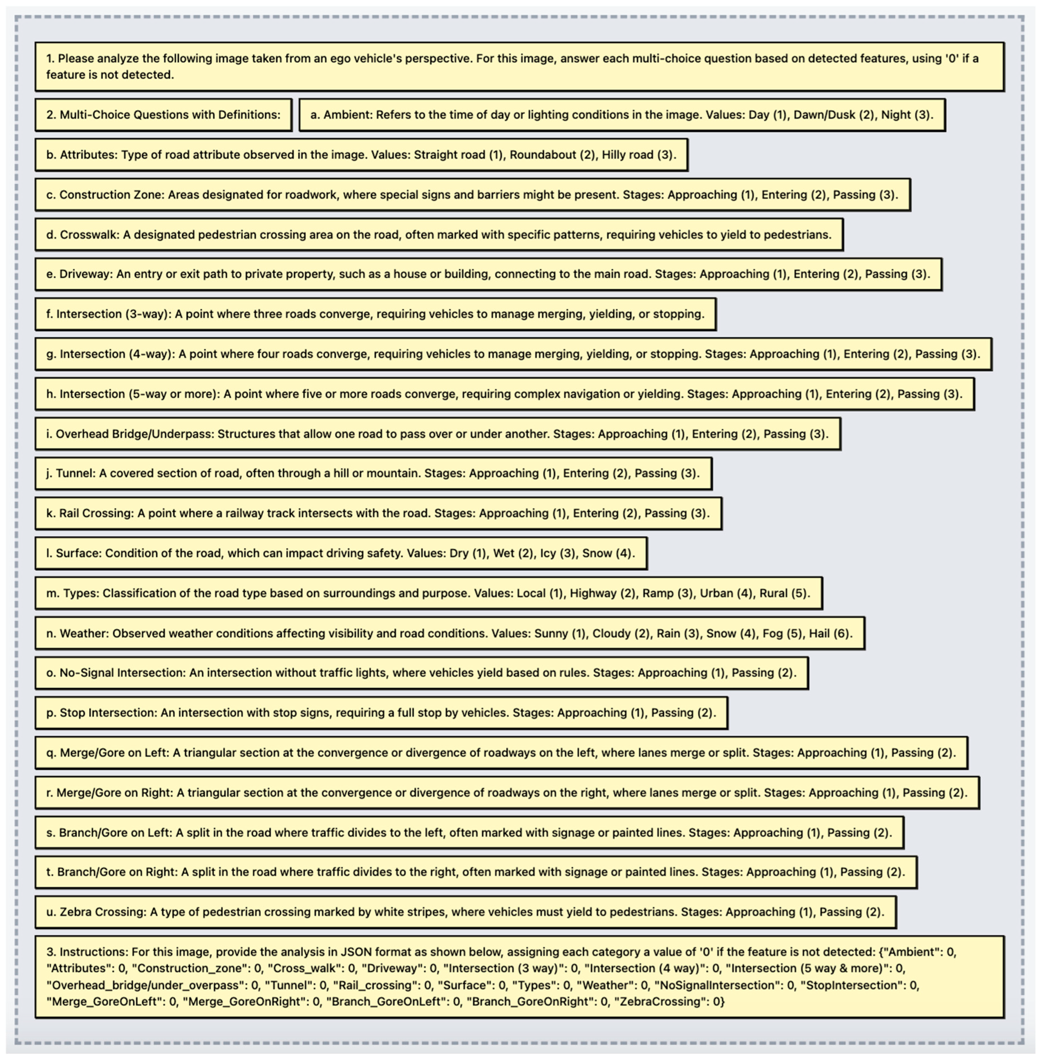
Our methodology is designed to evaluate various CLIP model variants across different numbers of nearest neighbors (NNs) and compare their performance against the baseline model, GPT-4o, in a zero-shot, in-context learning setting. Models are ranked based on their precision and recall performance across multiple attributes. The prompt is designed for GPT-4o to analyze driving-related images from the perspective of an ego vehicle and classify the detected features into predefined categories, as shown in Figure 3. It provides a structured framework for scene understanding by assigning values to categories such as road attributes, weather conditions, and complex road structures. Furthermore, we did not define terms like “gore” in the prompt, which refers to a triangular-shaped section of land where a road diverges or converges, commonly found at highway entry or exit ramps, as we relied on the model’s prior knowledge. However, compared to the CLIP retrieval system, this approach removes many attributes because the indexed images in this analysis represent only a single level or class. Additionally, temporal features like “Stages” (e.g., approaching, entering, passing) are converted into a binary format for simplicity. For instance, categories such as “Rail Crossing” are represented as “0” if not detected and as “1” if detected, effectively merging the temporal stages into a single binary outcome. This conversion aligns with the frame-based nature of the analysis in this paper, focusing on frame-level detection and classification rather than temporal sequences. This streamlined representation ensures the framework is optimized for frame-based image retrieval and analysis, critical for real-time and retrospective applications.
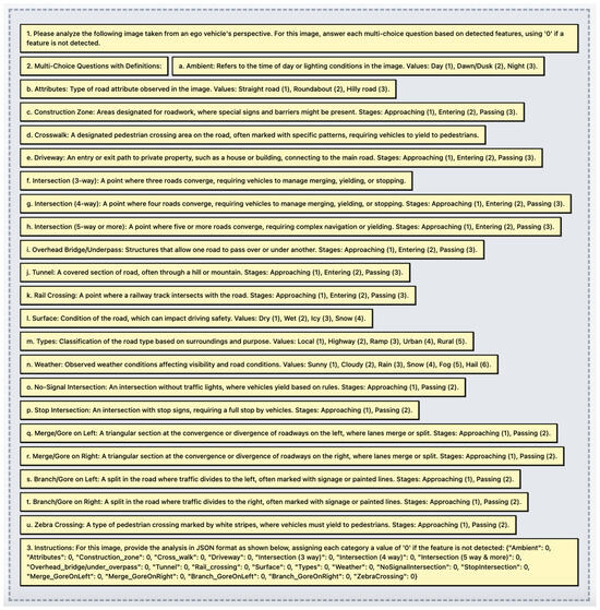
Figure 3.
Structured prompt for scene understanding by assigning values to categories such as road attributes, weather conditions, and complex road structures. The prompt shows all the attributes used to test the models.
6.2. Pretrained Models Results
In this section, we address the first research question: how well do pretrained models perform in the context of scene understanding? Our primary focus is to identify which of these relatively lightweight models, capable of real-time inference, achieve higher rankings compared to other CLIP models studied here and GPT-4o in zero-shot settings.
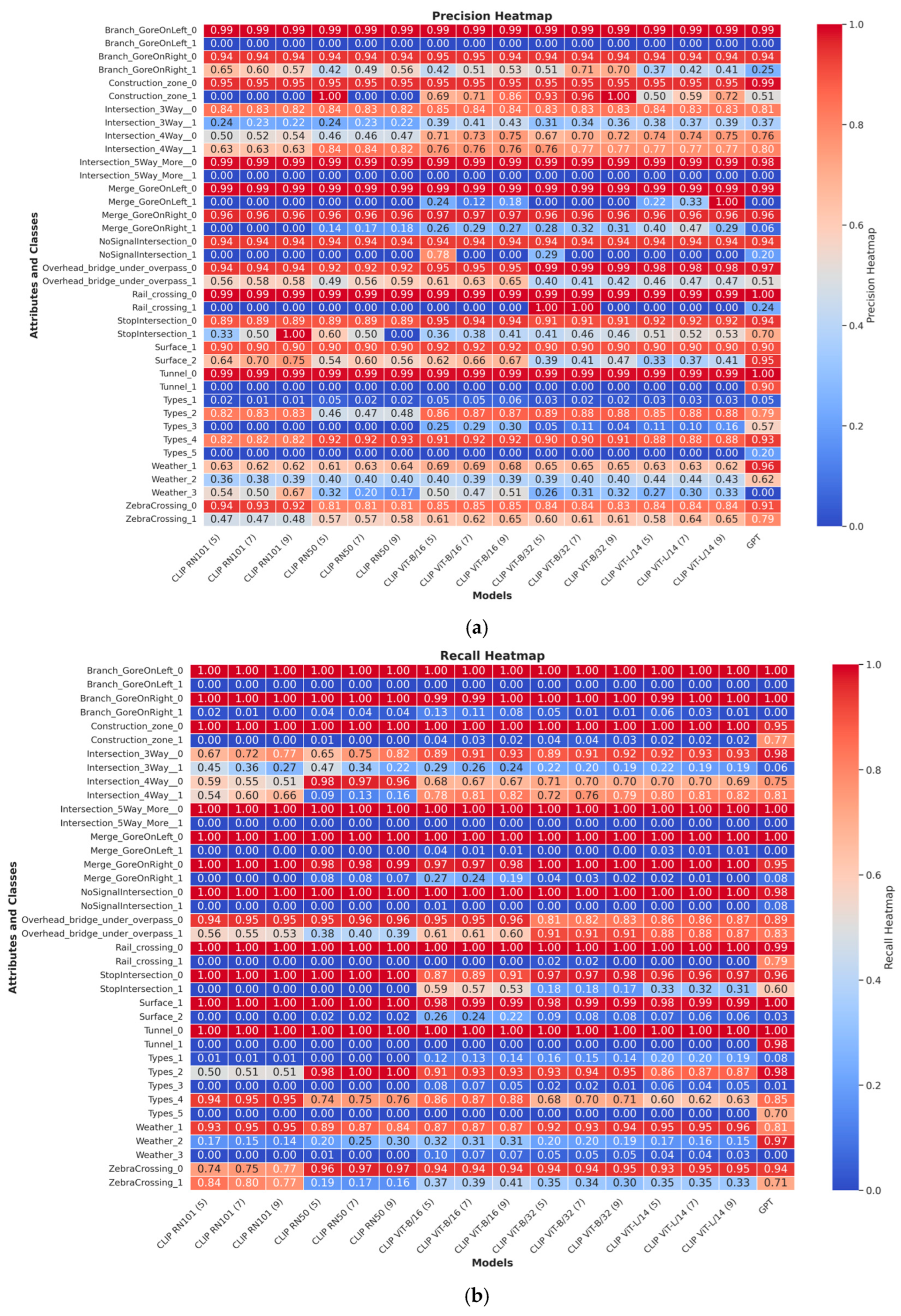
Given the inherent imbalance in the dataset, precision, recall, and F1-score are the most appropriate evaluation metrics, as they provide insights into how well models handle both majority and minority classes [28]. To this end, we evaluated the performance of these models in terms of precision, recall, and F1-score across different class levels, as shown in Figure 4, aiming to pinpoint their strengths and limitations. The heatmaps below illustrate the performance of different models across various attributes and classes using precision, recall, and F1-score. It is evident that the model performance varies significantly depending on the attribute and class, with notable disparities in the handling of minority classes. In general, the models struggle with minority classes, exhibiting lower recall and precision scores, which affects their overall F1-scores.
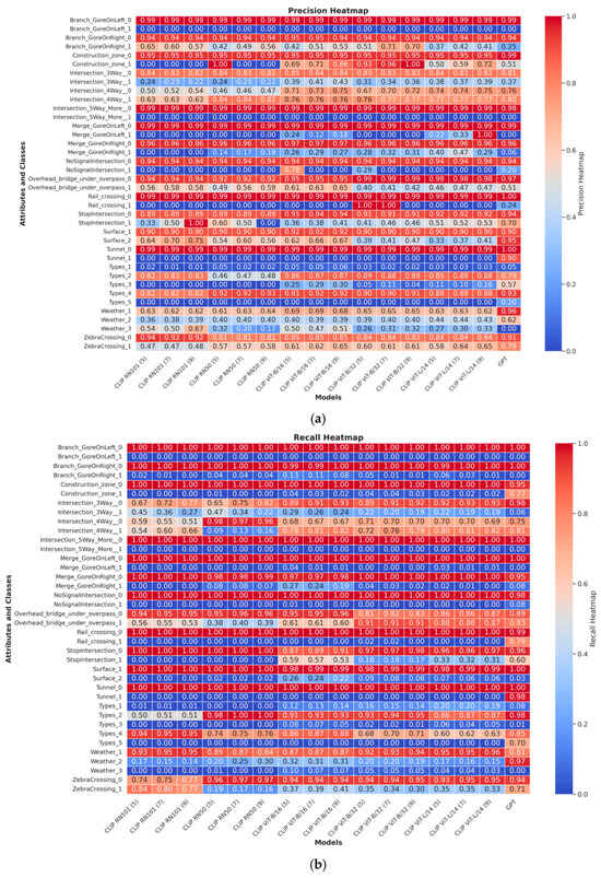
Figure 4.
The performance of different models across various attributes and classes using (a) precision, (b) recall, and (c) F1-score.
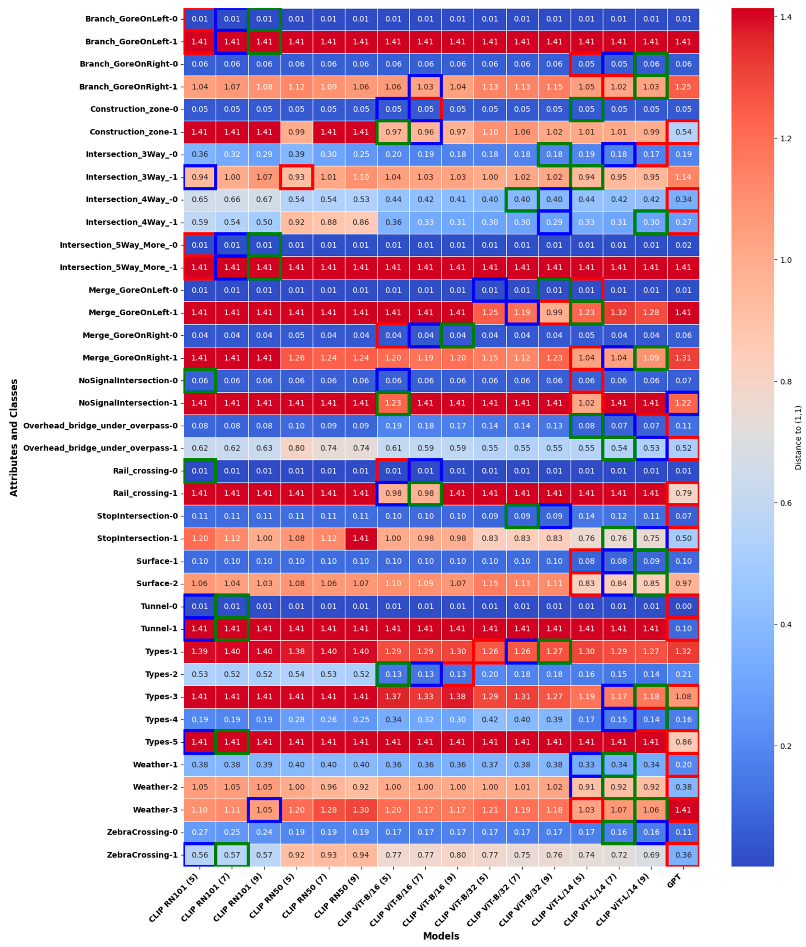
To ensure a robust comparison of model performance, we use the distance from the optimal (1,1) point in the precision–recall space as a basis for evaluation. This approach allows for a fairer assessment of how well a model balances precision and recall, especially in cases of class imbalance. Moreover, it provides a more intuitive 2D visualization for comparison while effectively preserving both recall and precision information. Based on that, we ranked the models using the Euclidean distance between their positions in the precision–recall space and the optimal (1,1) point, providing a clear metric for performance comparison. This distance serves as a metric for ranking the models, with smaller distances indicating better performance. For visualization, we present a heatmap where each cell represents the distance of a model for a specific attribute–class combination. It is important to note that the CLIP models used in this study rely on retrieval-based mechanisms, where the number of nearest neighbors (indicated in parentheses) is adjusted for each model. Once the best-performing CLIP models are identified, we proceed to the fine-tuning phase for further performance enhancement. These results are presented in Figure 5.
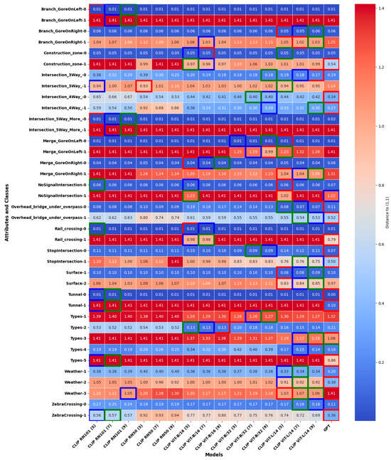
Figure 5.
Heatmap showing the pretrained model rankings based on Euclidean distance to the ideal precision–recall point (1,1) for all attribute–class combinations, with top-performing models highlighted. The models with the top three performances (smallest distances) for each attribute–class combination are highlighted with bounding boxes of different colors: green for the best, blue for the second-best, and red for the third-best.
Figure 5 presents the distance values, with the top-performing models highlighted based on their proximity to point (1). Additionally, when the distance values within the heatmap cells are identical, the order of the models should be disregarded. The GPT-4o model consistently ranks as one of the top-performing models across multiple attribute–class combinations, indicated by its frequent appearance with minimal distances. Similarly, CLIP ViT-B/32 (5) and CLIP ViT-L/14 (5)—where the number in parentheses indicates the number of approximate nearest neighbors’ models—exhibit strong performance in several cases, particularly for attributes such as “Merge_GoreOnLeft” and “ZebraCrossing”.
GPT-4o, as a zero-shot model, performs well in specific attributes, such as detecting the absence of construction zones, where it achieves balanced precision and recall. Meanwhile, the RN models (RN50 and RN101) exhibit lower overall performance compared to the CLIP models. These models tend to prioritize precision over recall, particularly in intersection scenarios, reflecting a conservative prediction strategy but with reduced sensitivity.
Attribute-specific trends further illustrate these differences. For Branch and Merge Gore scenarios, CLIP models outperform GPT-4o, maintaining moderate precision and recall, while GPT-4o shows substantial limitations in generalizing to complex spatial relationships. In the Construction Zone attribute, GPT-4o excels in detecting non-construction zones but performs inconsistently in construction-specific scenarios. Conversely, CLIP models show a greater deviation from the optimal precision–recall point in Class 1. For intersections, as the complexity increases from three-way to five-way scenarios, all models struggle, with ViT-L/14 achieving the best precision but sacrificing recall. In the Overhead Bridge/Underpass attribute, Class 0 scenarios see all models performing well, but for Class 1, ViT-L/14 strikes a balance between precision and recall, outperforming GPT-4o, which shows high recall but lower precision.
A clear trend emerges across all attributes: models perform significantly better in simpler scenarios (Class 0) compared to complex ones (Class 1). The CLIP models consistently outperform GPT-4o and RN models in handling complex spatial reasoning tasks, emphasizing their robustness for such applications. Additionally, a trade-off between precision and recall is evident, with ViT-L/14 prioritizing precision while other models, such as ViT-B/16 and GPT-4o, emphasize recall.
The analysis highlights the strengths of CLIP models, particularly the ViT variants, in delivering robust performance for complex scene understanding. GPT-4o, while commendable in simpler scenarios, is less reliable in domain-specific tasks. The observed trade-offs between precision and recall suggest that hybrid approaches or fine-tuning could further improve model performance, especially in dynamic and nuanced driving contexts.
6.3. Fine-Tuned Models Results
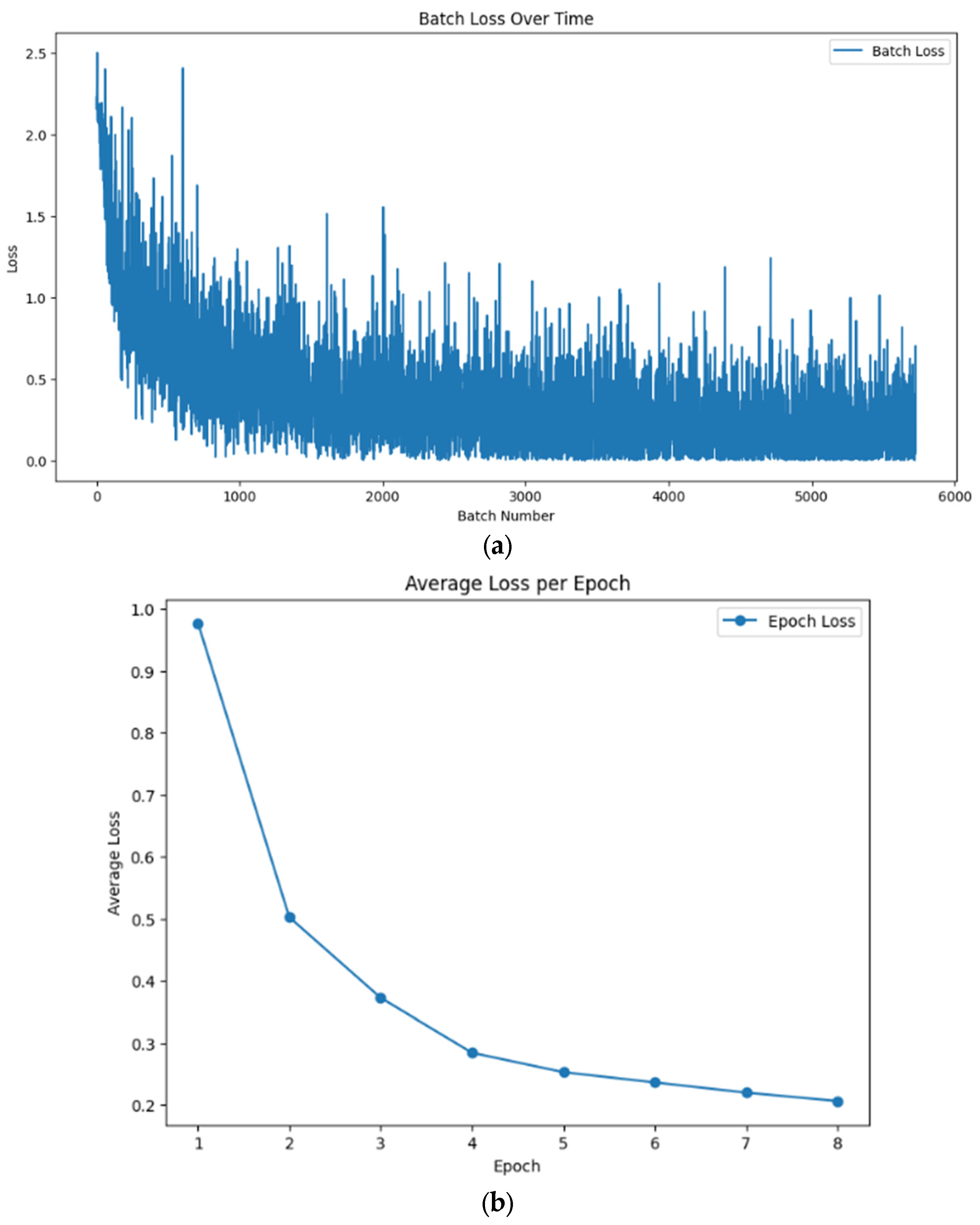
As CLIP ViT-B/32 (5) and CLIP ViT-L/14 (5) showed the best performance among all models, we chose to fine-tune them. The training data preparation involves pairing images with textual descriptions generated from associated attributes, extracted from CSV files. Each image is processed and matched with a descriptive text string representing its attributes to create input pairs for the model. The training process employs the Adam with a Weight Decay optimizer with a learning rate of 10−5. The model is trained over eight epochs using mixed-precision training to enhance computational efficiency. Performance is monitored by tracking loss values at both batch and epoch levels, as shown in Figure 6, ensuring consistent evaluation throughout the training.

Figure 6.
Performance is monitored by tracking loss values at both batch and epoch levels for the fine-tuned OpenAI CLIP ViT-L/14 model. Panel (a) plot illustrates batch loss over time, reflecting fluctuations with an overall downward trend, ensuring consistent evaluation throughout training. Panel (b) plot shows average loss per epoch, demonstrating a steady decrease in loss, indicating effective learning.
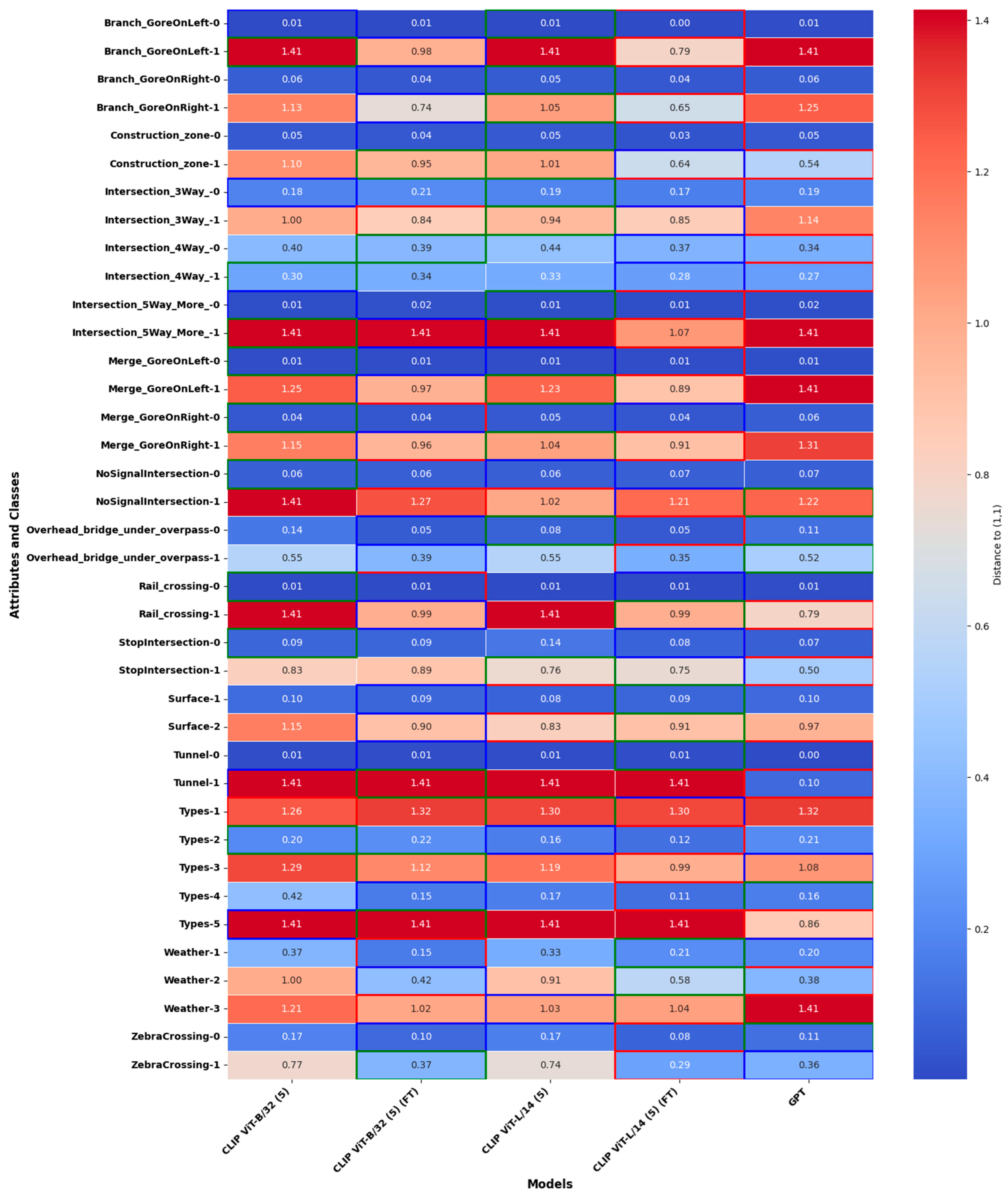
The heatmap In Figure 7 illustrates the distances between the precision–recall points of various models and the ideal point (1,1) in the precision–recall space, aggregated across attributes and scales. The performance of the models is represented with a color gradient, where lower distances (closer to blue) indicate better alignment with the ideal, and the top three performing models for each attribute–class pair are highlighted. The comparison of fine-tuned and non-fine-tuned CLIP ViT-B/32 (5) and CLIP ViT-L/14 (5) models, as well as GPT-4o in its zero-shot configuration, reveals key insights into model performance and adaptability.
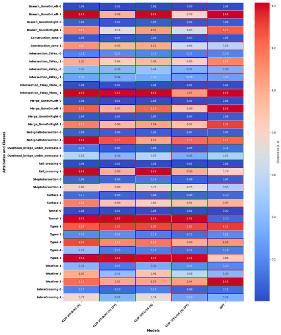
Figure 7.
Heatmap showing the performance improvement of fine-tuned models (FT) compared to non-fine-tuned counterparts and GPT-4o in zero-shot, highlighting top-performing models across attributes and scales. The models with the top three performances (smallest distances) for each attribute–class combination are highlighted with bounding boxes of different colors: green for the best, blue for the second-best, and red for the third-best.
The fine-tuned models of CLIP ViT-B/32 (5) and CLIP ViT-L/14 (5), which are labeled as FT in Figure 4, demonstrate consistent improvements over their non-fine-tuned counterparts. This is evident in their reduced distances across multiple attribute–class pairs, such as ZebraCrossing-1, Weather-2, and StopIntersection-1. Fine-tuning allows these models to adapt effectively to the nuances of the dataset, enhancing their precision and recall and bringing their performance closer to the ideal. This adaptability highlights the importance of leveraging fine-tuning to optimize lightweight models for specific tasks.
When compared to GPT-4o in its zero-shot configuration, the fine-tuned models frequently outperform or match its performance. For instance, CLIP ViT-L/14 (5) (FT) surpasses GPT-4o in attributes such as Types-2 and Tunnel-1, while CLIP ViT-B/32 (5) (FT) achieves competitive results in attributes like Merge GoreOnLeft-1 and Surface-2. This is particularly significant given GPT-4o’s reliance on large-scale pretraining, demonstrating that task-specific fine-tuning can enable lightweight models to rival or exceed the capabilities of more resource-intensive models.
7. Discussion
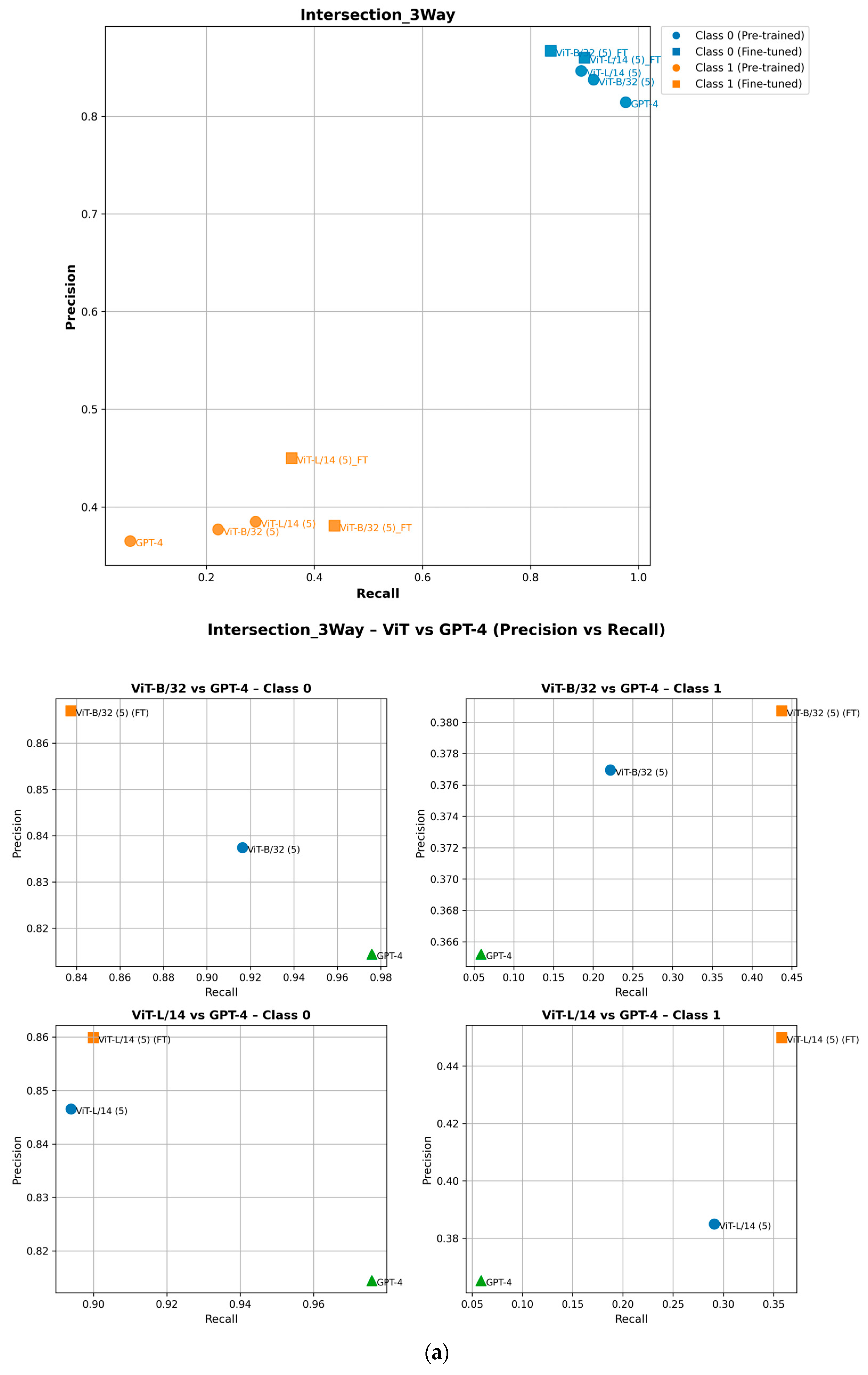
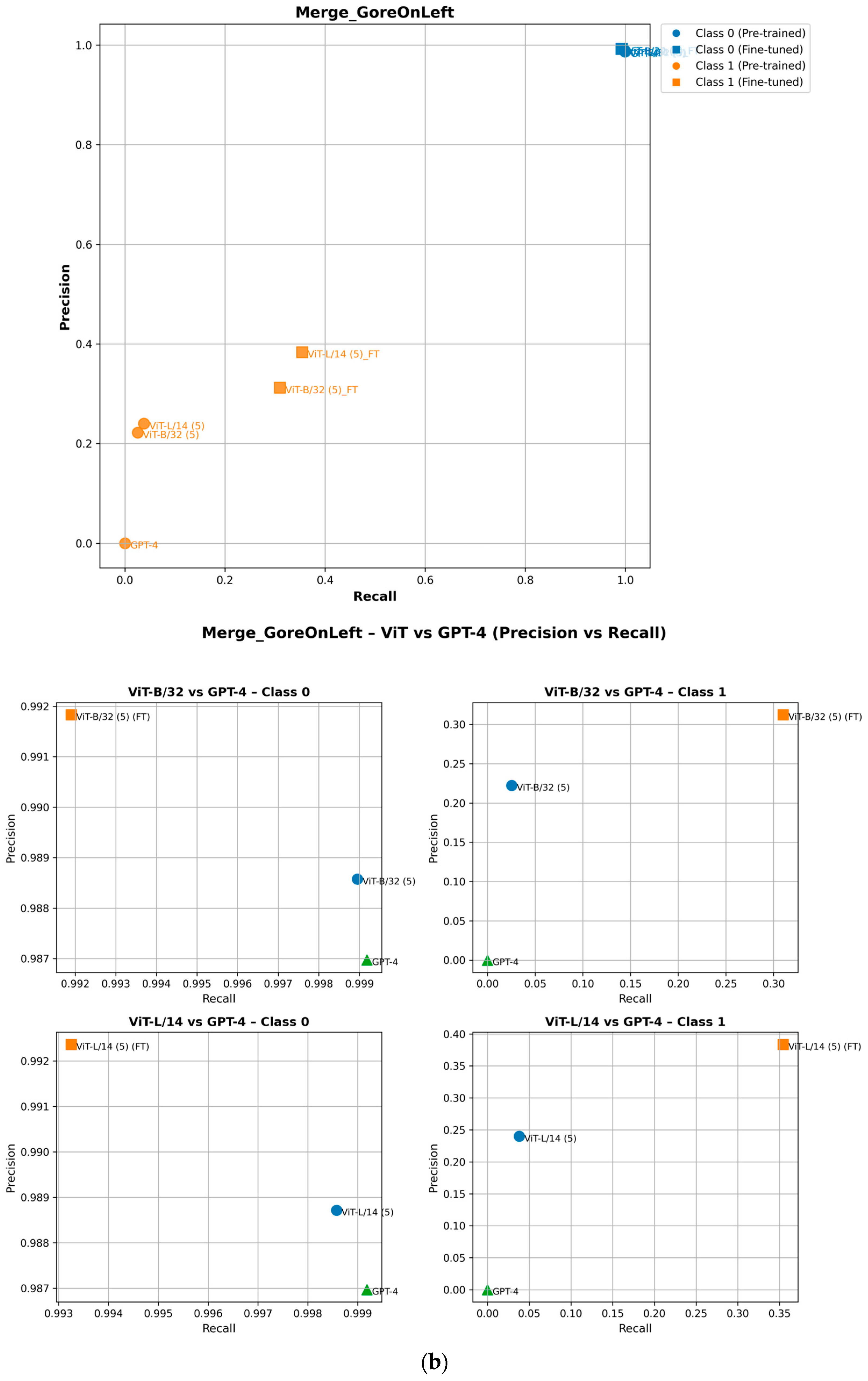
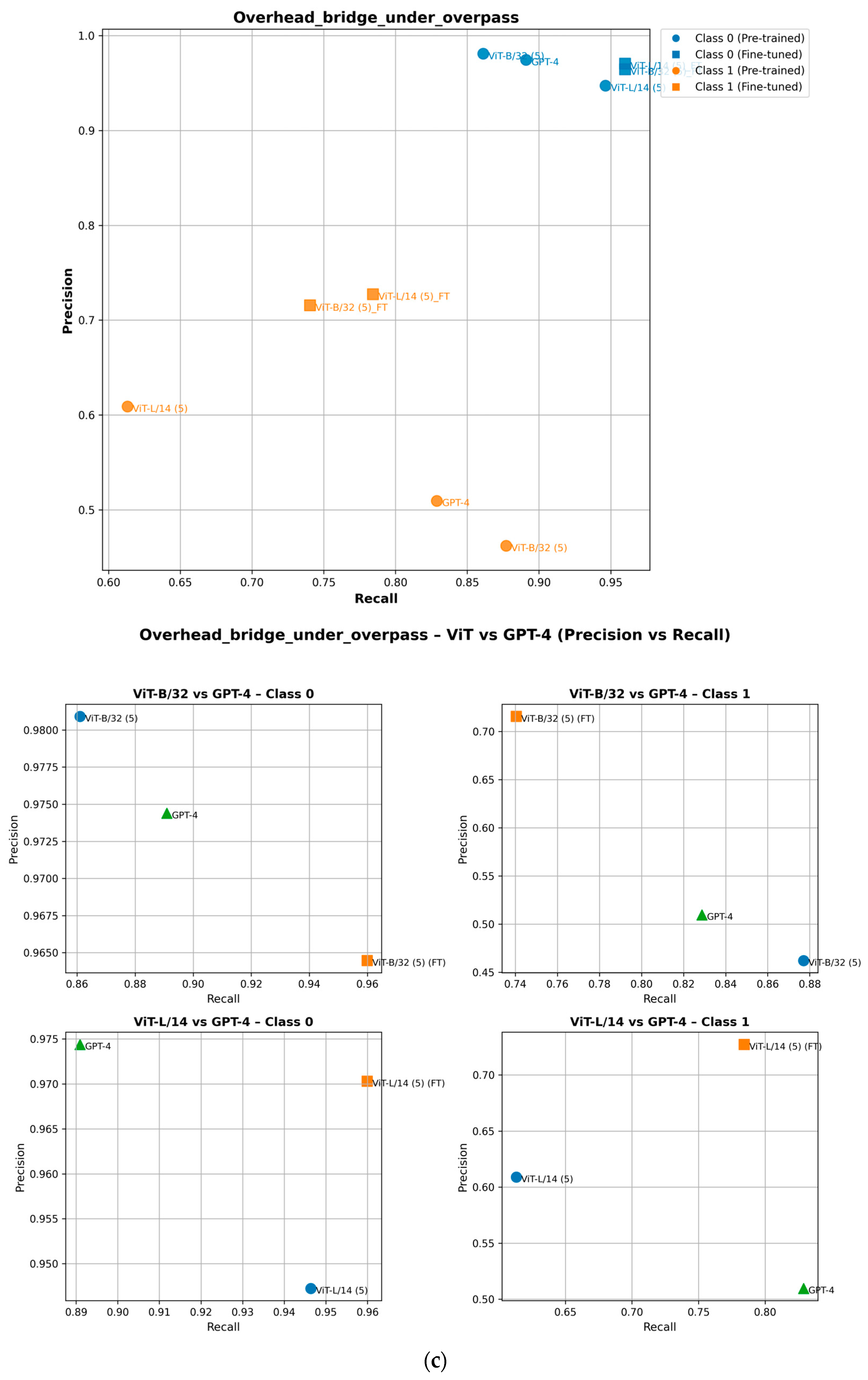
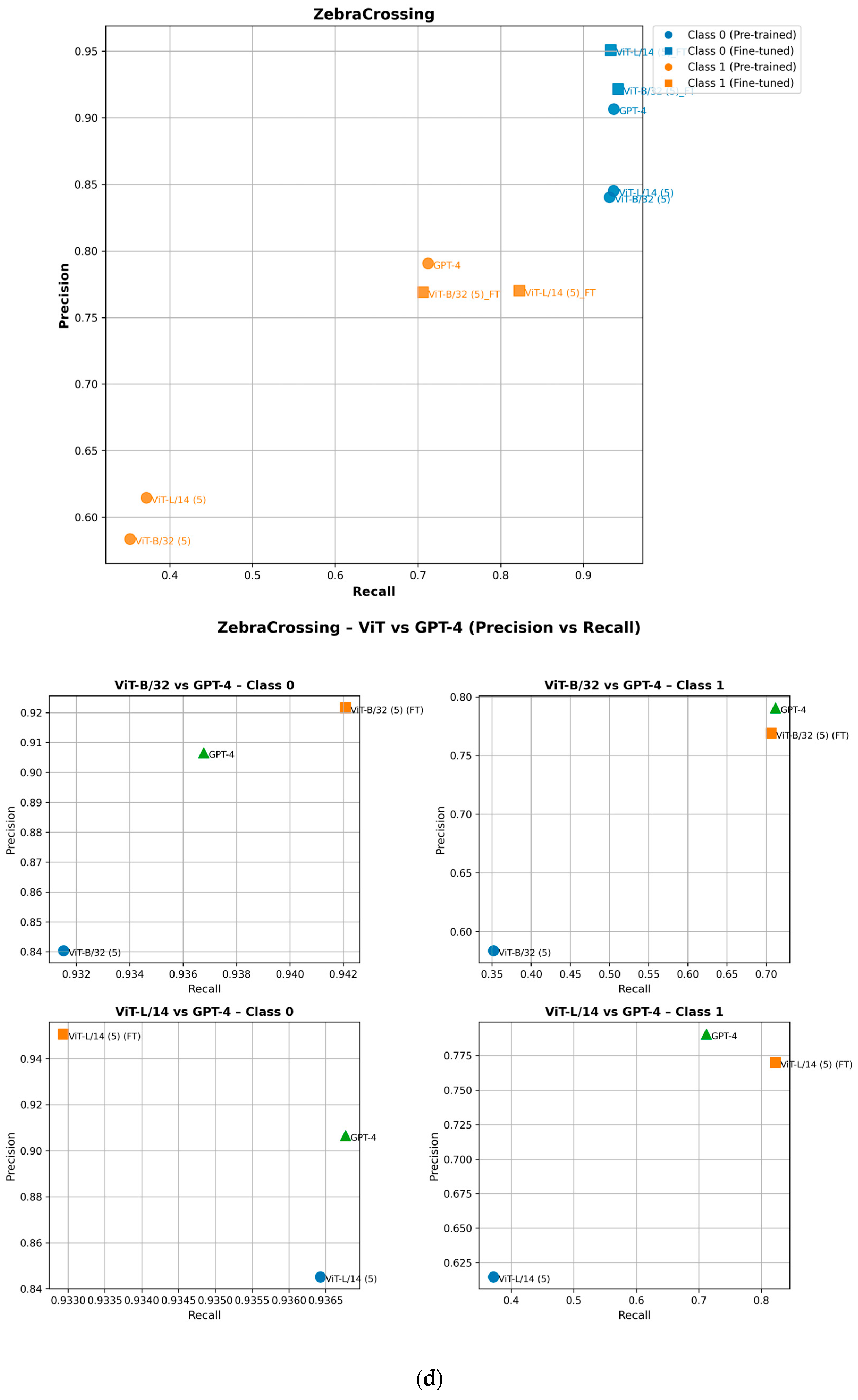
To ensure completeness, we analyze how fine-tuning improves the performance of minority class (Class 1) attributes in the precision–recall space. As shown in the precision–recall curves, fine-tuning shifts Class 1 data points upward, indicating improved precision, or rightward, reflecting higher recall [29]. For example, in the ZebraCrossing, Overhead_bridge_under_overpass, Merge_GoreOnLeft and Intersection_3Way attributes, fine-tuned models show an evident recall and precision gain, leading to better overall F1-scores [30]. This is shown in Figure 8. Importantly, this improvement does not negatively impact Class 0 (the majority class), which maintains its strong predictive performance, as seen in its consistent positioning across models. These findings highlight the effectiveness of fine-tuning in balancing model performance across the different classes.
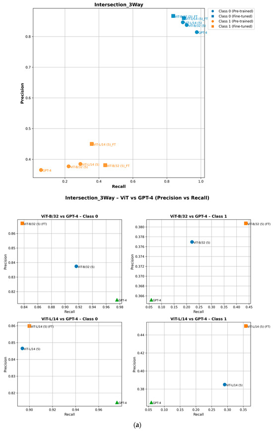


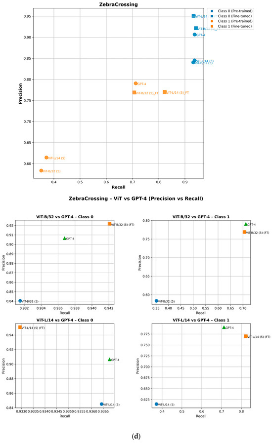
Figure 8.
Performance of pretrained and fine-tuned models in the precision–recall space for (a) Intersection_3Way, (b) Merge_GoreOnLeft, (c) Overhead_bridge_under_overpass, and (d) ZebraCrossing attributes.
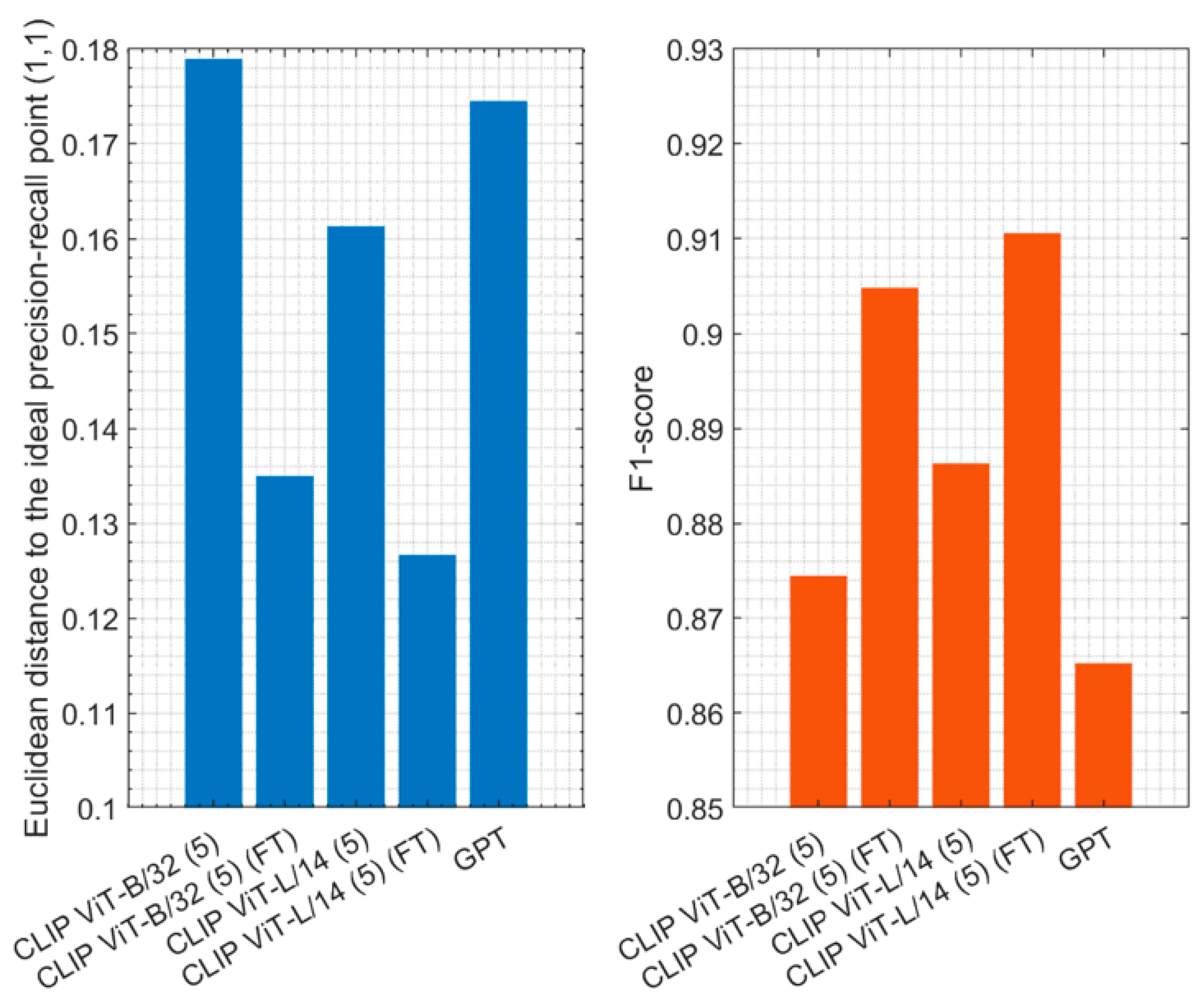
Finally, to make a direct comparison across all attributes, Figure 9 illustrates the aggregated performance of CLIP ViT-B/32 (5) and CLIP ViT-L/14 (5) with their fine-tuned counterparts and GPT-4o in zero-shot settings, measured using the mean of weighted precision, recall, and F1-scores. The results show the Euclidean distance to the ideal precision–recall point (1,1), where smaller values indicate better performance. Fine-tuned models exhibit significantly lower distances, demonstrating their improved alignment with the ideal point. The results of the F1-scores showed that CLIP ViT-L/14 (5) (FT) achieved the highest value of about 91.1%, followed by CLIP ViT-B/32 (5) (FT) with 90.5%, highlighting their careful balance between precision and recall. These results emphasize the effectiveness of fine-tuning in enhancing model performance compared to zero-shot or pretrained approaches.

Figure 9.
Aggregated performance of CLIP ViT-B/32 (5) and CLIP ViT-L/14 (5) with their fine-tuned counterparts and GPT-4o in zero-shot settings, measured using the mean of weighted precision, recall, and F1-scores.
The results underscore the potential of lightweight models like CLIP ViT-B/32 and CLIP ViT-L/14 for real-time deployment on edge devices. These models are computationally efficient, making them suitable for dynamic, resource-constrained environments such as ADASs or other autonomous vehicle systems. Fine-tuning further enhances their suitability by aligning their performance with specific datasets, ensuring both accuracy and efficiency in real-time applications.
In terms of practical deployment considerations, while our proposed models demonstrate promising performance in controlled environments, their deployment in actual vehicle systems presents additional challenges related to inference latency and power consumption. These factors are highly dependent on both software optimization techniques and the computational capabilities of the hardware used. For instance, real-time performance can be enhanced through model quantization, hardware acceleration (e.g., using GPUs or TPUs), and efficient memory management strategies. However, given the current stage of development, the technology readiness level (TRL) remains relatively low, indicating that further refinement is necessary before large-scale integration into commercial vehicular systems. Future work should focus on benchmarking these models on embedded automotive hardware, optimizing their efficiency for real-world deployment, and conducting field tests to assess their robustness under varying driving conditions.
8. Conclusions
This study presents a robust framework for real-time scene understanding in leveraging the capabilities of the CLIP model, which can be used for real-time deployment on edge devices. A CLIP-based retrieval system was fine-tuned for real-time ADAS applications, enabling the accurate classification of dynamic driving scenes. The model was benchmarked against state-of-the-art in-context learning methods, including GPT-4o in zero-shot scenarios, where it demonstrated superior performance, particularly in complex scenarios. Comprehensive frame-level evaluations were conducted using the Honda Scenes Dataset, which includes 80 h of annotated driving videos capturing diverse road and weather conditions. These evaluations highlighted the robustness of the framework across varied environments. Additionally, the integration of language-based supervision with visual scene recognition enhanced the semantic understanding of traffic scenes, contributing valuable insights to road safety and autonomous driving research.
By embedding scene images into a high-dimensional vector space using CLIP and indexing them with FAISS, the framework enabled the rapid and precise retrieval of relevant scenes. This feature is critical for real-time ADAS applications. Fine-tuning the CLIP models, such as ViT-L/14 and ViT-B/32, improved their performance by aligning embeddings with the semantic requirements of scene understanding. Notably, the fine-tuned ViT-L/14 model achieved the highest F1-score of 91.1%, followed closely by ViT-B/32 at 90.5%.
The precision and recall analysis revealed trade-offs between these metrics, with different models emphasizing either precision (e.g., ViT-L/14) or recall (e.g., ViT-B/16). This finding underscores the need to select models based on the specific requirements of a given application. The lightweight nature of models like ViT-B/32 and ViT-L/14, combined with their computational efficiency, positions them as ideal candidates for deployment on edge devices in resource-constrained environments, such as autonomous vehicles.
As fine-tuning significantly enhanced the models’ ability to classify complex scenes, this positions CLIP as a scalable, accurate, and efficient solution for dynamic scene understanding. Furthermore, the study’s exploration of multimodal techniques, including advanced indexing and semantic-rich embeddings, provides a solid foundation for future advancements in AI-driven scene classification systems.
Practically, this study establishes a pathway toward safer, smarter, and more context-aware autonomous driving systems. The integration of advanced techniques and models, like CLIP, ensures precise, real-time decision-making capabilities, enabling more effective ADAS and paving the way for further innovations in autonomous vehicle technology.
However, our study has some limitations. The evaluation was conducted on a single dataset (Honda Scenes), which may not fully represent all driving conditions. Additionally, while FAISS-based retrieval proved efficient, the model lacks sequential awareness, which could impact performance in dynamically evolving traffic scenarios. Future work will focus on enhancing generalization through broader dataset validation and real-world deployment testing.
Author Contributions
Conceptualization, M.E., H.I.A., A.R., T.I.A., A.J. and M.A.T.; methodology, M.E., H.I.A., A.R., T.I.A., A.J. and M.A.T.; software, M.E. and H.I.A.; validation, M.E. and H.I.A.; formal analysis, M.E., H.I.A., A.R., T.I.A., A.J. and M.A.T.; investigation, M.E. and H.I.A.; writing—original draft preparation, M.E., H.I.A., A.R., T.I.A., A.J. and M.A.T.; writing—review and editing, M.E., H.I.A., A.R., T.I.A., A.J. and M.A.T.; visualization, M.E. and H.I.A.; supervision, M.E. and H.I.A. All authors have read and agreed to the published version of the manuscript.
Funding
This research was funded partially by the Australian Government through the Australian Research Council Discovery Project DP220102598.
Data Availability Statement
Data are available upon request from the corresponding author.
Acknowledgments
We appreciate the partially foundation of the Australian Government through the Australian Research Council Discovery Project DP220102598.
Conflicts of Interest
The authors declare no conflicts of interest.
References
- Ramanishka, V.; Chen, Y.-T.; Misu, T.; Saenko, K. Toward driving scene understanding: A dataset for learning driver behavior and causal reasoning. In Proceedings of the IEEE Conference on Computer Vision and Pattern Recognition, Salt Lake City, UT, USA, 18–23 June 2018; pp. 7699–7707. [Google Scholar]
- Ashqar, H.I.; Alhadidi, T.I.; Elhenawy, M.; Khanfar, N.O. Leveraging Multimodal Large Language Models (MLLMs) for Enhanced Object Detection and Scene Understanding in Thermal Images for Autonomous Driving Systems. Automation 2024, 5, 508–526. [Google Scholar] [CrossRef]
- Yang, J.; Liu, C.; Chu, P.; Wen, X.; Zhang, Y. Exploration of the relationships between hazard perception and eye movement for young drivers. J. Adv. Transp. 2021, 2021, 6642999. [Google Scholar]
- Khanfar, N.O.; Elhenawy, M.M.; Ashqar, H.I.; Hussain, Q.; Alhajyaseen, W.K. Driving behavior classification at signalized intersections using vehicle kinematics: Application of unsupervised machine learning. Int. J. Inj. Control. Saf. Promot. 2023, 30, 34–44. [Google Scholar] [CrossRef]
- Khan, S.S.; Shen, Z.; Sun, H.; Patel, A.; Abedi, A. Supervised Contrastive Learning for Detecting Anomalous Driving Behaviours from Multimodal Videos. In Proceedings of the 2022 19th Conference on Robots and Vision (CRV), Toronto, ON, Canada, 31 May–2 June 2022. [Google Scholar]
- Ping, P.; Qin, W.; Xu, Y.; Miyajima, C.; Takeda, K. Impact of driver behavior on fuel consumption: Classification, evaluation and prediction using machine learning. IEEE Access 2019, 7, 78515–78532. [Google Scholar] [CrossRef]
- Masello, L.; Sheehan, B.; Castignani, G.; Shannon, D.; Murphy, F. On the impact of advanced driver assistance systems on driving distraction and risky behaviour: An empirical analysis of irish commercial drivers. Accid. Anal. Prev. 2023, 183, 106969. [Google Scholar] [CrossRef] [PubMed]
- Niu, S.; Ma, Y.; Wei, C. Night-time lane positioning based on camera and LiDAR fusion. In Proceedings of the Sixth International Conference on Traffic Engineering and Transportation System (ICTETS 2022), Guangzhou, China, 23–25 September 2022; SPIE: Bellingham, WA, USA, 2023; pp. 362–367. [Google Scholar]
- Orlovska, J.; Novakazi, F.; Wickman, C.; Söderberg, R. Mixed-method design for user behavior evaluation of automated driver assistance systems: An automotive industry case. In Proceedings of the Design Society International Conference on Engineering Design, Delft, The Netherlands, 5–8 August 2019; pp. 1803–1812. [Google Scholar] [CrossRef]
- DeGuzman, C.; Ayas, S.; Donmez, B. Limitation-focused versus responsibility-focused advanced driver assistance systems training: A thematic analysis of driver opinions. Transp. Res. Rec. J. Transp. Res. Board 2023, 2677, 122–132. [Google Scholar] [CrossRef]
- Tami, M.A.; Ashqar, H.I.; Elhenawy, M.; Glaser, S.; Rakotonirainy, A. Using Multimodal Large Language Models (MLLMs) for Automated Detection of Traffic Safety-Critical Events. Vehicles 2024, 6, 1571–1590. [Google Scholar] [CrossRef]
- Pradhan, A.; Hungund, A.; Pai, G.; Pamarthi, J. How does training influence use and understanding of advanced vehicle technologies: A simulator evaluation of driver behavior and mental models. Traffic Saf. Res. 2023, 3, 000024. [Google Scholar] [CrossRef]
- Palac, D.; Scully, I.; Jonas, R.; Campbell, J.; Young, D.; Cades, D. Advanced driver assistance systems (ADAS): Who’s driving what and what’s driving use? In Proceedings of the Human Factors and Ergonomics Society Annual Meeting, Baltimore, MD, USA, 3–8 October 2021; pp. 1220–1224. [Google Scholar] [CrossRef]
- Guo, J.; Wang, J.; Wang, H.; Xiao, B.; He, Z.; Li, L. Research on Road Scene Understanding of Autonomous Vehicles Based on Multi-Task Learning. Sensors 2023, 23, 6238. [Google Scholar] [CrossRef] [PubMed]
- Zhou, X.; Liu, M.; Zagar, B.L.; Yurtsever, E.; Knoll, A.C. Vision language models in autonomous driving and intelligent transportation systems. arXiv 2023, arXiv:2310.14414. [Google Scholar]
- Pham, T.; Do, T.; Sünderhauf, N.; Reid, I. Scenecut: Joint geometric and object segmentation for indoor scenes. In Proceedings of the IEEE International Conference on Robotics and Automation (ICRA), Brisbane, Australia, 21–25 May 2018. [Google Scholar] [CrossRef]
- Li, L.; Ota, K.; Dong, M. Sustainable cnn for robotic: An offloading game in the 3d vision computation. IEEE Trans. Sustain. Comput. 2019, 4, 67–76. [Google Scholar] [CrossRef]
- Ni, J.; Shen, K.; Chen, Y.; Cao, W.; Yang, S. An improved deep network-based scene classification method for self-driving cars. IEEE Trans. Instrum. Meas. 2022, 71, 1–14. [Google Scholar] [CrossRef]
- Guo, Z.; Huang, Y.; Hu, X.; Wei, H.; Zhao, B. A survey on deep learning based approaches for scene understanding in autonomous driving. Electronics 2021, 10, 471. [Google Scholar] [CrossRef]
- Dosovitskiy, A. An image is worth 16x16 words: Transformers for image recognition at scale. arXiv 2020, arXiv:2010.11929. [Google Scholar]
- Radford, A.; Kim, J.W.; Hallacy, C.; Ramesh, A.; Goh, G.; Agarwal, S.; Sastry, G.; Askell, A.; Mishkin, P.; Clark, J. Learning transferable visual models from natural language supervision. In Proceedings of the International Conference on Machine Learning, Virtual, 18–24 July 2021; pp. 8748–8763. [Google Scholar]
- Han, C.; Li, H.; Xu, J.; Dong, B.; Wang, Y.; Zhou, X.; Zhao, S. Unbiased 3D semantic scene graph prediction in point cloud using deep learning. Appl. Sci. 2023, 13, 5657. [Google Scholar] [CrossRef]
- Li, C.; Yan, F.; Wang, S.; Zhuang, Y. A 3d lidar odometry for ugvs using coarse-to-fine deep scene flow estimation. Trans. Inst. Meas. Control 2022, 45, 274–286. [Google Scholar] [CrossRef]
- Vernekar, P.; Singh, A.; Patil, K. Pothole and wet surface detection using pretrained models and ml techniques. Int. J. Res. Appl. Sci. Eng. Technol. 2023, 11, 626–633. [Google Scholar] [CrossRef]
- Holst, D.; Schoepflin, D.; Schüppstuhl, T. Generation of synthetic ai training data for robotic grasp-candidate identification and evaluation in intralogistics bin-picking scenarios. In Proceedings of the International Conference on Flexible Automation and Intelligent Manufacturing, Detroit, MI, USA, 19–23 June 2022; pp. 284–292. [Google Scholar] [CrossRef]
- Zipfl, M.; Zöllner, J. Towards traffic scene description: The semantic scene graph. In Proceedings of the IEEE Intelligent Transportation Systems Conference (ITSC), Macau, China, 8–12 October 2022. [Google Scholar] [CrossRef]
- He, K.; Zhang, X.; Ren, S.; Sun, J. Deep residual learning for image recognition. In Proceedings of the IEEE Conference on Computer Vision and Pattern Recognition, Las Vegas, NV, USA, 27–30 June 2016; pp. 770–778. [Google Scholar]
- Saito, T.; Rehmsmeier, M. The precision-recall plot is more informative than the ROC plot when evaluating binary classifiers on imbalanced datasets. PLoS ONE 2015, 10, e0118432. [Google Scholar]
- Prexawanprasut, T.; Banditwattanawong, T. Improving Minority Class Recall through a Novel Cluster-Based Oversampling Technique. Informatics 2024, 11, 35. [Google Scholar] [CrossRef]
- Samad, S.R.A.; Balasubaramanian, S.; Al-Kaabi, A.S.; Sharma, B.; Chowdhury, S.; Mehbodniya, A.; Webber, J.L.; Bostani, A. Analysis of the Performance Impact of Fine-Tuned Machine Learning Model for Phishing URL Detection. Electronics 2023, 12, 1642. [Google Scholar] [CrossRef]

Disclaimer/Publisher’s Note: The statements, opinions and data contained in all publications are solely those of the individual author(s) and contributor(s) and not of MDPI and/or the editor(s). MDPI and/or the editor(s) disclaim responsibility for any injury to people or property resulting from any ideas, methods, instructions or products referred to in the content. |
© 2025 by the authors. Licensee MDPI, Basel, Switzerland. This article is an open access article distributed under the terms and conditions of the Creative Commons Attribution (CC BY) license (https://creativecommons.org/licenses/by/4.0/).