Abstract
Time series forecasting is extensively utilised in meteorology, transportation, finance, and industrial domains. Precisely recognising cyclical trends and abrupt local changes in time series is essential for enhancing forecasting accuracy. Frequency-domain representations are adept at identifying periodic traits, whereas time-domain approaches are superior for spotting localised quick changes. Traditional techniques sometimes prioritise a single domain, overlooking the advantages of integration. This paper introduces a novel hybrid model, FFTNet, that simultaneously pulls characteristics from both domains to optimise their respective benefits. Theoretical examination indicates that the 2D CNN utilises dual-axis convolution kernels to jointly describe global cross-patch structures and local temporal patterns, whilst the frequency-domain MLP enhances spectral components in accordance with Parseval’s Theorem and the Convolution Theorem. A frequency-domain MLP is employed to discern periodic and trend characteristics, while a 2D CNN in the time domain identifies localised abrupt changes. This hybrid methodology differentiates itself from previous methods that depend exclusively on a single domain, providing a more thorough comprehension of the underlying patterns in time series data. Experiments on seven real-world datasets indicate that FFTNet surpasses existing techniques, attaining state-of-the-art performance with enhancements of 11.8% and 4.7% in MSE and MAE, respectively.
1. Introduction
Time series forecasting is a mathematical technique used to predict future trends based on present data. Given a set of multivariate time series samples , where each sample at time step is a vector of dimension , and with a look-back window , the objective is to predict the following values . Time series forecasting is crucial in various practical applications, such as meteorological prediction [1], traffic flow analysis [2], financial forecasting [3], and market trend analysis [4]. This technique enables the forecasting of future occurrences by the analysis of historical data and trends, providing decision assistance for individuals and organisations, reducing risks, optimising resource allocation, and improving operational efficiency. Owing to its substantial practical importance, an increasing number of scholars have started to focus on this field [5].
Accurately capturing dynamic variations in temporal data is crucial for developing effective time series forecasting models. Progress in deep learning technologies has resulted in the extensive application of models utilising convolutional neural networks (CNNs) [6,7], multilayer perceptrons (MLPs) [8,9,10], recurrent neural networks (RNNs) [11,12], and Transformers [13,14] for time series analysis. Notwithstanding the considerable accomplishments of these models in time series forecasting, their discrepancies in feature extraction and representation reveal potential for future optimisation. A comprehensive method that amalgamates the strengths of many models is crucial for in-depth comprehension and forecasting of time series data. Particular emphasis should be placed on evaluating a model’s efficacy in terms of both its temporal performance and its capacity to discern periodic features in the frequency domain. Some models directly analyse time series data in the time domain [6], while others investigate its periodic properties in the frequency domain [10], with both approaches yielding significant results. Various models, however, discern distinct patterns in time series data across temporal and frequency domains, influencing both the model’s understanding of the data and its predictive effectiveness.
For example, as demonstrated in Figure 1(left). The feature map of time series data analysed by a frequency-domain MLP reveals that the feature values are primarily spread, with only a few areas nearing zero. This distribution illustrates that the MLP effectively captures the periodicity and trends of the time series inside the frequency domain. Conversely, Figure 1(right) illustrates the feature map of the same time series analysed by a CNN, displaying a contrasting pattern: most feature values are near zero, with only a few regions exhibiting increased values. This sparse distribution suggests that CNN is more inclined to focus on local and significant changes in the time series, such as trend shifts or anomalies. Given these differences, we propose modelling time series data by incorporating information from both the frequency and time domains. This thorough approach may enhance the understanding and predictive precision of the time series data.
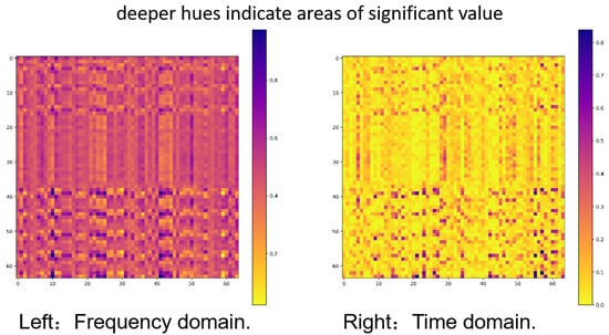
Figure 1.
The depiction of feature maps from MLP in the frequency domain and CNN in the time domain demonstrates unique patterns. The left image illustrates a uniform distribution of feature values, emphasising the benefit of the frequency-domain MLP in capturing long-term periodic characteristics. Conversely, the right image displays a more sparse feature distribution, suggesting that the CNN is more responsive to transient and localised variations in time series data.
Inspired by the previously mentioned findings, this study introduces a novel frequency–time hybrid architecture, FFTNet, which integrates Frequency and Temporal Awareness for long-term time series forecasting. FFTNet comprises three fundamental components: the Local-Context ConvBlock (LCCB), the Global-Cyclic Recogniser (GCR), and the Frequency–Time Aggregation Block (FTAB), designed to capture both local and global trends in time series data.
This paper outlines several significant contributions. We commence with a thorough review of the distinctions between time-domain and frequency-domain approaches in temporal feature extraction. Our data suggest that time-domain methods are most sensitive to localised sudden changes, whereas frequency-domain methods excel at detecting periodic and trend features. This comprehensive understanding provides a solid theoretical foundation for our subsequent research. Secondly, we provide a unique frequency-time hybrid architecture named FFTNet, specifically designed for long-term time series forecasting. FFTNet enhances prediction accuracy and processing efficiency through the skilful integration of Frequency and Temporal Awareness. This innovative architecture represents a substantial advancement in the field of time series forecasting. We validate the superiority of our proposed technique by extensive testing on widely used real-world long-term forecasting benchmarks. The results demonstrate that FFTNet achieves state-of-the-art performance in Mean Squared Error (MSE) and Mean Absolute Error (MAE) metrics. Ablation studies demonstrate that the combined application of time and frequency domains significantly improves predicting performance. The findings illustrate the effectiveness and viability of FFTNet. The source code is accessible to the public at https://github.com/mackery/FFTNet.git (accessed on 23 March 2025).
2. Related Work
2.1. Time Domain Methods
Conventional time series forecasting techniques, such as ARMA [15] and ARIMA [16], predominantly rely on linear assumptions, hence constraining their capacity to accurately identify nonlinear patterns and intricate connections within data. In recent years, the advancement of deep learning techniques has resulted in the advent of methods that provide substantial benefits in this field. Transformer-based approaches, including LogTrans [17], Informer [18], Autoformer [19], PyraFormer [13], and PatchTST [20], have attained significant success in time series forecasting, mostly owing to their self-attention mechanisms. RNN-based approaches, such as those referenced in [12,21,22,23] and SegRNN [11], have garnered interest due to their network architectures that excel in capturing temporal dependencies in sequential data.
Furthermore, techniques utilising multi-layer perceptrons (MLPs), such as [24], that delineate intricate dependencies incrementally, together with TimeMixer [25], MTS-Mixers [26], and TSMixer [9], amalgamate univariate and cross-variable characteristics. Simultaneously, Dlinear [8] and TiDE [27] utilise channel-independent processes, both attaining outstanding outcomes. Temporal convolutional networks (TCNs) [6] encapsulate an extensive perspective on time series, encompassing variations and trends, through the amalgamation of local features and global correlations. Alternative methodologies [28] suggest architectures that utilise recursive down-sampling, convolution, and interaction to maintain temporal linkages, even post-down-sampling.
Despite advancements in time-domain methods for capturing local characteristics and dynamic changes in time series, they encounter challenges in addressing periodic patterns and long-range interdependence. This has compelled researchers to investigate approaches based on the frequency domain.
2.2. Frequency Domain Methods
Frequency domain methods for time series forecasting effectively utilise the periodic and frequency components inherent in time series data. Recently, various forecasting methodologies have been established to derive insights from the frequency domain for predictive purposes. StemGNN [29] integrates graph Fourier transform (GFT) and discrete Fourier transform (DFT) to concurrently represent correlations and temporal dependencies within time series. SFM [30] transforms the concealed states of LSTM into the frequency domain via DFT. CoST [31] utilises DFT to transform intermediate information into the frequency domain and executes convolution to identify the periodic elements of time series. FiLM [32] uses Fourier analysis to preserve collected data while eliminating noise signals. FreTS [10] presents a specialised MLP architecture that analyses the real and imaginary components of frequency coefficients. FITS [33] employs FFT to convert time series into the frequency domain, utilising a complicated linear layer architecture in conjunction with a low-pass filter to mitigate the effects of high-frequency noise.
While frequency-domain approaches are proficient in identifying periodic characteristics, they frequently neglect short-term dependencies and local dynamics in time series data, hence limiting their efficacy in accurately representing the intricate complexity inherent in such datasets.
2.3. Hybrid Time–Frequency Methods
Moosavi [34] utilised wavelet transformation as a preprocessing method to amalgamate the time and frequency domains in the historical development of time–frequency integration. The Wavelet–ANFIS model was developed by combining wavelet processing with ANFIS, facilitating accurate predictions of groundwater levels. Joo [35] proposed a forecasting method based on wavelet filtering, enabling simultaneous analysis of time series data in both time and frequency domains. The original time series was broken into trend and variation components via wavelet filtering, therefore, effectively extracting characteristics across several domains.
N-BEATS [36] tackles the attributes of seasonality, including its systematic, cyclical, and repetitive variations. It uses the Fourier series as the foundational function to represent seasonality. Furthermore, it utilises the notion of double residual stacking in conjunction with forecasting and backcasting for predictive purposes. ATFN [37] maps the spectrum of the current sliding window to that of the prediction interval. A multi-layer neural network performs a transformation similar to the inverse discrete Fourier transform to generate predictions of periodic features. FEDformer [38] presents a frequency improvement module utilising discrete Fourier transform (DFT) and discrete wavelet transform (DWT). This framework adeptly directs the network in acquiring time–domain characteristics by seizing various intervals of the input sequence inside the frequency domain. The method proposed by Wu [7] utilises periodicity derived from the frequency domain to improve the extraction of periodic characteristics in the time domain. The PDF [39] encapsulates multiple intervals of the input sequence into the frequency domain to enhance the efficacy of two-dimensional CNNs in extracting time-domain characteristics. PathFormer [40] utilises DFT and IDFT to extract time-series periodicity within its multi-scale routing module, including trend decomposition for multi-scale modelling. However, its straightforward use cannot leverage the potential of the frequency domain.
Our solution, FFTNet, diverges from previous approaches that depend on frequency-domain information to facilitate the learning of time-domain features. The FFTNet models time series by amalgamating frequency-domain and time-domain information, employing a Global-Cyclic Recogniser (GCR) in the frequency domain to capture periodicity and long-range dependencies, while utilising a TCN-based Local-Context ConvBlock (LCCB) in the time domain to identify local variations. This design enables the efficient recognition of both long-term and short-term patterns in time series data.
3. Methodology
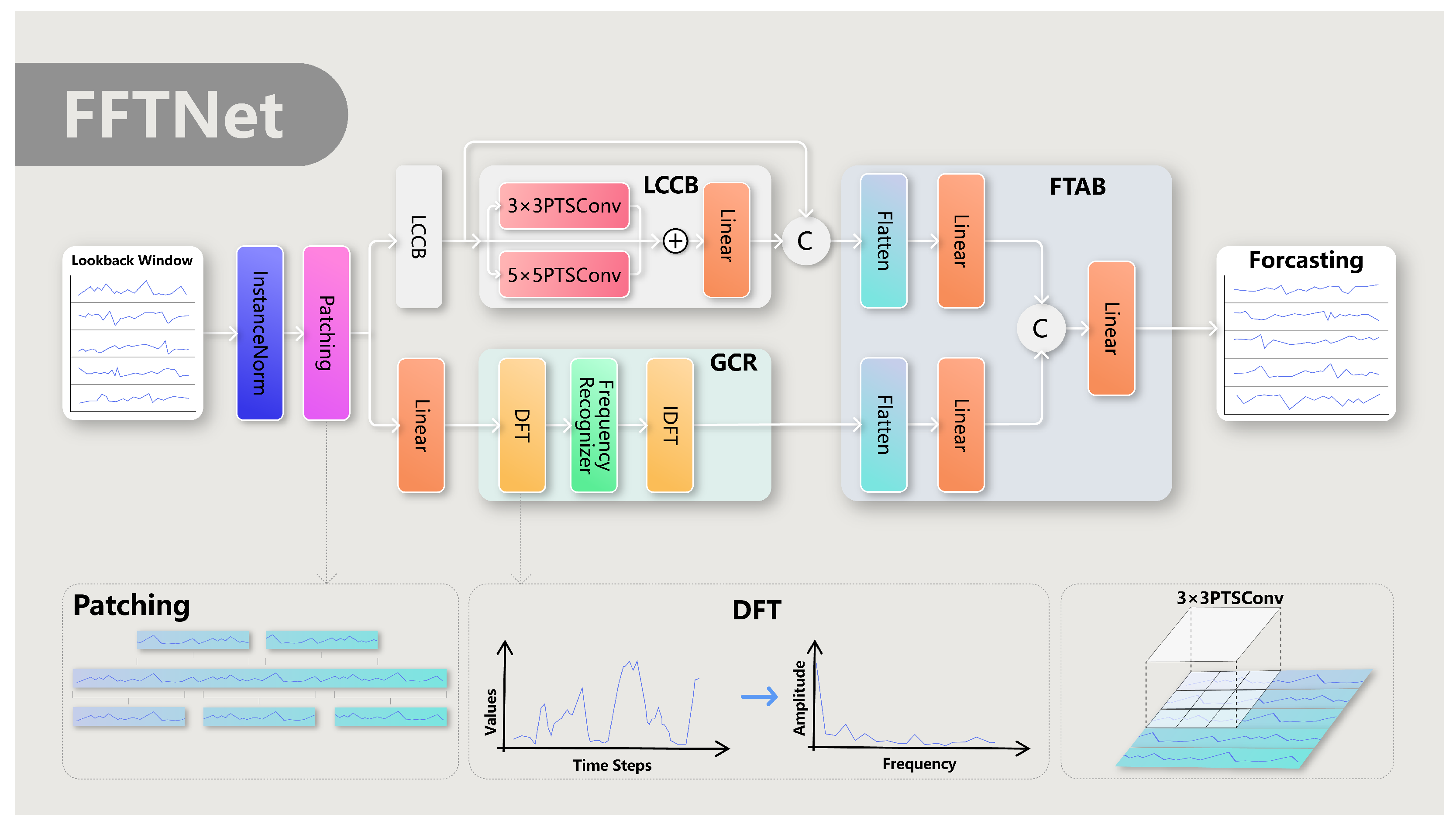
The comprehensive architecture of the FFTNet model’s design is influenced by the twin attributes of time series data: sudden local variations and cyclical trends. To simultaneously address both problems, FFTNet employs a hybrid feature extraction technique that amalgamates frequency-domain and time-domain data. The model, illustrated in Figure 2, comprises three primary components: the Local-Context ConvBlock (LCCB), the Global-Cyclic Recogniser (GCR), and the Frequency–Time Aggregation Block (FTAB).

Figure 2.
The overall architecture of FFTNet.
The Local-Context ConvBlock (LCCB) captures local dynamics and short-term relationships in time series data. It accomplishes this by dividing the time series into successive sub-sequence patches and utilising a two-dimensional convolutional neural network (2D CNN) to identify these local variances. The Global-Cyclic Recogniser (GCR) emphasises the detection of periodic and trend attributes of time series through a frequency-domain analysis. Utilising the discrete Fourier transform (DFT) to transform segmented time series data into the frequency domain and employing a frequency-domain multilayer perceptron (MLP) for the analysis and extraction of periodic features, the GCR effectively captures long-term dependencies and global patterns within the time series. The Frequency–Time Aggregation Block (FTAB) is engineered to proficiently amalgamate the local and global features derived from the LCCB and GCR. The FTAB integrates features from several viewpoints using flattening, linear projection, and concatenation operations, equipping the model with a thorough comprehension of the underlying behaviours in the time series.
3.1. Patching
We employ the patching idea [20] to convert the input time series into a collection of patches for analysis. Define the matrix as the input time series, where denotes the number of channels, and signifies the sequence length. The matrix is subsequently transformed into a Temporal Patch Tensor , where denotes the quantity of patches. When , overlapping elements arise across contiguous patches.
Takens’ theorem [41] states that the phase space reconstruction of a time series is accomplished by delay embedding.
, which represents the t-th column of the phase space , preserves the dynamical properties of the original system, facilitating nonlinear prediction. Let m represent the embedding dimension and denote the delay time. Subsequently, we will examine the Patching approach, which demonstrates strong correlations with phase space reconstruction in time series analysis. Each patch corresponds to a local time interval , which is analogous to picking observations with a particular time offset in the delay embedding. Overlapping patches, created by varying step sizes S and lengths P, establish a hierarchical time-delay framework akin to phase space analysis with numerous embedding dimensions. The intersection of patches creates dependencies across neighbouring time periods, analogous to the correlation of delayed coordinates in the Takens theorem. Taking into account the delayed embedding matrix in phase space reconstruction, we have
When the sliding step size of patching is and the patch length is , the unfolded matrix of the patch tensor exhibits the same spatial structure as , thereby demonstrating the equivalence of the two in phase space representation. Patching, via structured temporal window segmentation and overlapping design, is mathematically analogous to localised phase space reconstruction techniques.
3.2. Comparing 2D CNNs vs. 1D CNNs
The proposed architecture, which is based on 2D convolutional neural networks (CNNs), is constructed upon the tensor representation , obtained from patching operations. Its theoretical superiority over 1D CNNs is grounded in two fundamental mechanisms.
The 2D convolution kernel , where pertains to the dimension associated with the original N-axis for inter-patch operations and corresponds to the dimension related to the original P-axis for intra-patch temporal operations, simultaneously operates along both the inter-patch dimension (the N-axis) and the intra-patch temporal dimension (the P-axis). This dual-axis processing gives rise to significant characteristics. Specifically, the kernel weights function as learnable correlators. Here, the m-indexed weights are responsible for modelling the relationships between adjacent patches, which represent the global context, while the n-indexed weights capture the temporal patterns within individual patches, that is, the local context. Additionally, the effective receptive field can be dynamically adjusted by choosing the appropriate kernel size. This enables the unified modelling of multi-scale temporal dependencies without the need for structural cascading.
The weight-sharing mechanism in 2D convolution is formally presented as follows:
In this formula, denotes the output feature map at layer l and position . The variable C represents the number of input channels. and are the sizes of the 2D convolution kernel along the two axes, as previously defined. m and n serve as indices for summation within the kernel. is the weight of the convolution kernel at layer l, for channel c, and at position within the kernel. is the input tensor at layer , for channel c, at position , and is the bias term at layer l. This formulation offers two theoretical advantages in comparison to 1D CNNs. The dimension encodes cross-patch structural priors, adhering to the stationarity assumption, while the dimension maintains local temporal continuity. This effectively avoids the entangled feature learning that occurs in pure 1D operations. Single-layer kernels are capable of achieving hierarchical feature extraction through the independent control of (which determines the context scale) and (which defines the temporal granularity). In contrast, 1D CNNs necessitate explicit depth stacking to achieve similar effects.
3.3. Frequency MLP vs. Time-Domain MLP
Parseval’s Theorem states that for an original time series, if we denote its representation as T and let be the frequency components corresponding to the spectrum, the energy of a time series in the time domain is equal to the energy of its representation in the frequency domain. Formally, we can express this using the following notation:
where , v is the time dimension, and f is the frequency dimension. This theorem indicates that if most of the energy of a time series is concentrated in a small number of frequency components, then the time series can be accurately represented using only these components. Thus, discarding the others will not significantly affect the signal energy. Kun et al. [10] pointed out that in the frequency domain, the energy is concentrated in a smaller part of the frequency components, so learning in the spectrum can help maintain clearer patterns.
According to the Convolution Theorem, the element-wise multiplication operation of the Fourier transform in the frequency domain has an equivalent mapping relationship with the circular convolution operation in the discrete time domain. Based on this principle, the operation process of the frequency multilayer perceptron (Frequency MLP) can be mathematically characterised from the dual perspectives of the time–frequency domain: In the frequency domain, it is manifested as a linear modulation process of the spectrum components, while in the time domain, it is equivalent to a circular convolution operation. Specifically, given an input signal and its discrete Fourier transform , the Frequency MLP modifies the signal spectrum by designing a frequency-domain filter to generate an output signal . This process can be formally expressed as:
where ⊙ represents the Hadamard product and ⊛ is the circular convolution operator.
From the perspective of operator theory, the Frequency MLP is essentially a learnable spectral domain modulator. Its core function is to dynamically adjust the spectral characteristics of the input signal through the frequency-domain response function : For any frequency component , the filter coefficient applies an amplitude modulation factor and a phase shift , thus reconstructing the frequency-domain distribution of the output signal. This mechanism endows the Frequency MLP with the following key characteristics: It can enhance or suppress specific frequency components by parameterising ; the circular convolution operation ensures the covariance of time-domain translation operations; the numerical implementation based on the fast Fourier transform (FFT) supports end-to-end gradient optimisation.
In time series prediction tasks, the spectral modulation ability of the Frequency MLP can effectively decouple the multi-scale components in the signal. By adaptively adjusting the energy distribution of different frequency bands, this model can suppress high-frequency noise interference while enhancing the low-frequency trend terms and periodic terms that are strongly correlated with the prediction target, thereby improving prediction accuracy. Experimental studies show that such frequency-domain operators have better spectral resolution and parameter efficiency than traditional time-domain neural networks in non-stationary time series modelling [42].
In time series modelling, there are significant differences between the frequency multilayer perceptron (Frequency MLP) and the traditional time-domain multilayer perceptron (Time-domain MLP) in signal processing mechanisms, modelling capabilities, and task adaptability. The Time-domain MLP directly performs a point-wise non-linear transformation (such as a fully-connected layer) on the original time-domain signal . Its implicit assumption is that the local or global dependencies between time points can be explicitly modelled through stacked linear layers and activation functions. However, the Time-domain MLP has difficulty effectively separating the mixed multi-scale components (such as trends, cycles, and noise) in the signal. Especially in non-stationary time series, the coupling of high-frequency noise and low-frequency trends can lead to overfitting or underfitting of the model. By projecting the signal onto the frequency domain through the Fourier transform, explicit modulation (enhancing/suppressing specific frequency bands) of the spectral components is carried out using the frequency-domain filter . Based on the energy conservation theorem (), frequency-domain operations can decouple components without losing signal energy. For example, it can suppress high-frequency noise components while retaining low-frequency trends, thus improving the model’s ability to extract the essential features of the signal. In terms of computational complexity, the parameter complexity of the Time-domain MLP grows quadratically with the sequence length (), while the Frequency MLP, combined with the Fast Fourier Transform (FFT, with a complexity of ), can model long-range dependencies at a lower computational cost, especially for sequences with significant periodic or seasonal components. The dense weight matrix of the fully-connected layer in the Time-domain MLP requires a large number of parameters (, where d is the dimension of the hidden layer) to cover all time-point combinations, which is prone to overfitting and has poor interpretability (it is difficult to associate weights with specific time patterns).
The number of parameters of the frequency-domain filter is only related to the frequency resolution (usually ); each parameter directly corresponds to the gain/phase adjustment of a specific frequency component. For example, the modulus of , , reflects the model’s attention to the k-th frequency component and has a clear physical meaning. The main differences are summarised in Table 1 in this paper.

Table 1.
Difference between Frequency-domain MLP and Time-domain MLP.
3.4. Local-Context ConvBlock (LCCB)
The proposed Local-Context ConvBlock (LCCB) module is intended to effectively capture the spatial structural characteristics of time series data within convolutional neural networks (CNNs) and autonomously learn short-term relationships and patterns. The input time series is transformed into a Temporal Patch Tensor , with each element denoting a collection of local features associated with a certain time step. The LCCB module utilises two sets of convolutional kernels of varying dimensions, namely 3 × 3 and 5 × 5, applied to by grouped convolution. This design allows the network to extract local features at various sizes, with the 3 × 3 kernel emphasising tiny details and the 5 × 5 kernel detecting broader contextual information. Padding values of 1 and 2 are utilised for the 3 × 3 and 5 × 5 kernels, respectively, to uphold dimensional consistency and preserve the spatial dimensions of the feature maps following convolution processes.
Subsequent to the convolutional layers, a Gaussian Error Linear Unit (GeLU) activation layer [37] is included to provide nonlinearity and augment the model’s capacity to discern intricate patterns. To enhance the model’s ability to learn complex temporal patterns, residual learning is utilised by including the input into the output of the two convolutional layers prior to its transmission to a linear layer. Subsequent to the linear layer, an activation layer and a dropout layer are included to enhance nonlinearity and regularisation, mitigating the likelihood of overfitting. The LCCB module incorporates residual connections, promoting efficient gradient propagation in deep networks and improving sensitivity to fluctuations across various time scales. The module is defined and expressed by the subsequent formula:
In this context, and signify the 3 × 3 and 5 × 5 convolution operations, respectively, whereas denotes the linear layer. , denotes the feature dimension, signifies the number of patches, and indicates the patch size.
We utilise a dual-layer Local-Context ConvBlock (LCCB) architecture with feature fusion enabled by skip connections to augment the model’s representational ability for time series data. The dual-layer LCCB structure comprises two LCCB modules, each utilising the aforementioned convolution and activation processes. A skip connection is established between these two modules, connecting the output of the first LCCB layer to the input of the second LCCB layer. This architecture not only retains detailed features from the bottom layer but also improves the abstraction and integration of these elements through the subsequent processing of the second LCCB layer. This configuration can be represented as follows:
Here, denotes the concatenation of input tensors along the feature dimension, and represents the output from the first LCCB layer.
3.5. Global-Cyclic Recogniser (GCR)
The Global-Cyclic Recogniser (GCR) is engineered to identify long-term dependencies and global patterns in time series via frequency-domain transformation. The discrete Fourier transform (DFT) is utilised for the rapid conversion of time-domain data into the frequency domain. The time-domain input is converted into the frequency-domain by the subsequent formula:
Here, represents the -th component in the frequency domain, and is the -th sample in the time domain, where = 0, 1, 2, ; and is the imaginary unit. The DFT transforms the time-domain signal of the time series into the spectrum , which encapsulates information regarding the signal’s frequencies and amplitudes. This data, expressed as a synthesis of cosine and sine waves, encapsulates the periodic attributes of the time series. To further examine these frequency components, we employ a frequency MLP (designated as the ’Frequency Recogniser’ in this context) that learns the interactions between frequencies and their combined impact on the overarching behavioural patterns of the time series.
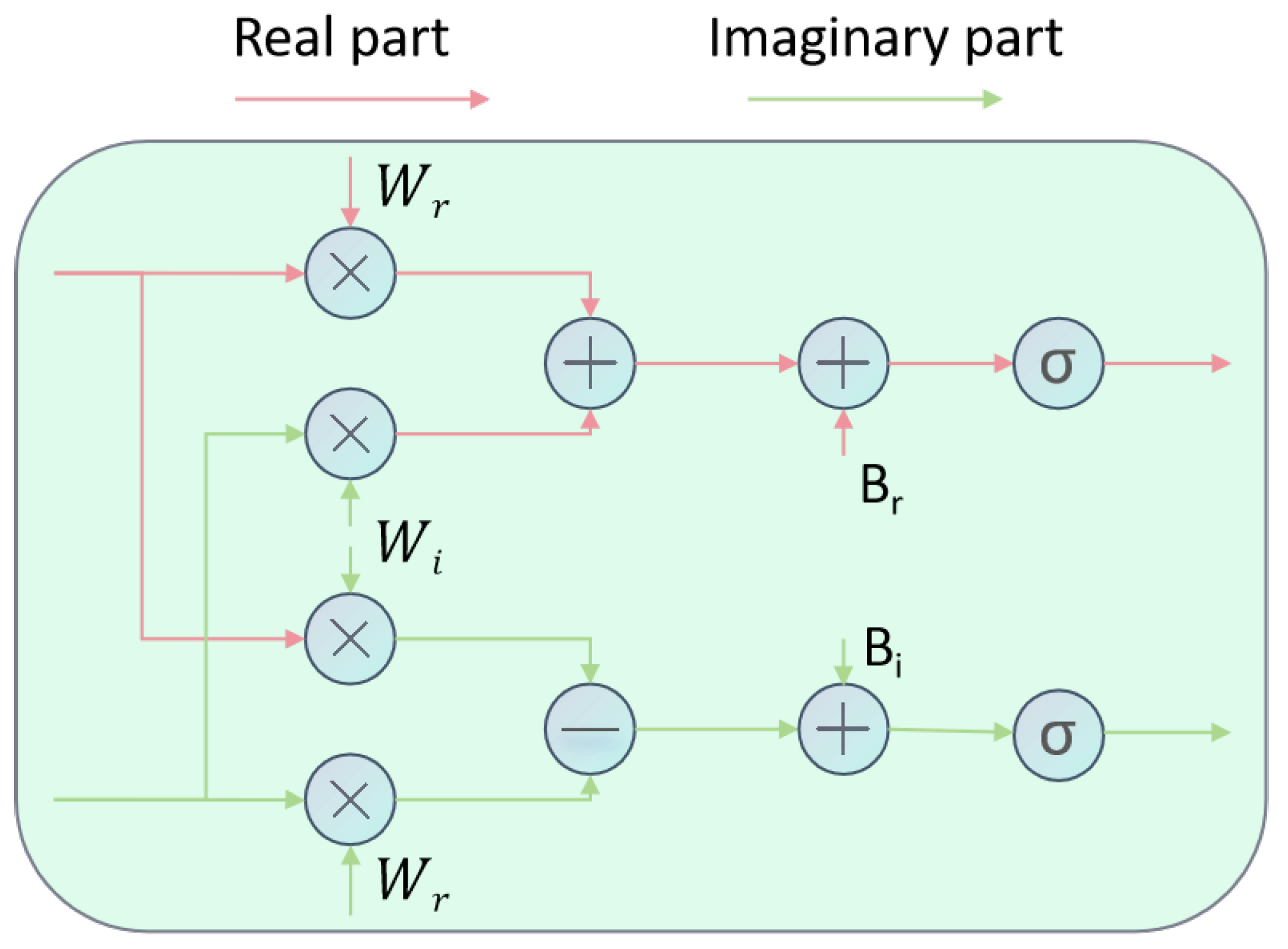
The Frequency Recogniser’s learning process can be articulated by the subsequent formula:
Here, signifies the complex output, is a soft-thresholding activation operation and represents the real and imaginary components of the weights, and denote the real and imaginary components of the input complex number X, and and indicate the real and imaginary components of the bias. Figure 3 clearly depicts the learning process of this formula. Upon concluding the learning process in the frequency domain, the signal is reverted to the time domain utilising the subsequent inverse transformation formula:
The principal benefit of the GCR method is its capacity to markedly improve the identification of global periodic characteristics in time series. The model efficiently extracts and learns global patterns from the frequency domain by integrating GCR. The GCR technique functions autonomously across many channels while sharing weights among the C channels, hence assuring parameter efficiency and computational optimisation.
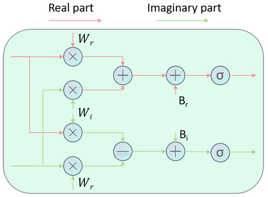
Figure 3.
Learning process of frequency recogniser.
The procedure commences with a slicing operation on the time series, as elucidated in Section 3.2, transforming it into a Temporal Patch Tensor. This stage disaggregates the time series into several segments, each containing localised temporal data. Subsequently, a linear layer encodes these patches, generating an encoded time series Z, with each element signifying a detailed feature representation of its corresponding temporal patch.
The encoded time series Z is derived as follows:
Here, , where D signifies the encoding dimension, indicates the number of patches, and each element pertains to the holistic feature representation of the -th temporal patch. = 0, 1, 2, …, − 1. The learning process of GCR can be articulated using the following formula:
Here, and signify the Fourier transform and inverse Fourier transform operations executed along the PatchNum dimension of the encoded time series Z; W denotes the complex weight matrix, B indicates the complex bias, and is the output reverted to the time domain.
3.6. Frequency Time Aggregation Block (FTAB)
Section 3.4 and Section 3.5 present the Local-Context ConvBlock (LCCB) and Global-Cyclic Recogniser (GCR), respectively. These modules generate the Local-Context feature and the Global-Cyclic feature using carefully crafted feature extraction processes. Specifically, emphasises the detection of nuanced fluctuations in the time series, whereas represents the overarching trend and cyclical patterns. The Frequency-Time Aggregation Block (FTAB) amalgamates these two feature types for efficient prediction.
The primary role of the FTAB module is to accept and as inputs and produce the prediction outcome. The initial step in this procedure is to consolidate the dimensions of these features by combining the final two dimensions of each feature tensor into one dimension. The mathematical representation of this dimension-reduction operation is as follows:
Here, Y represents the feature tensor designated for flattening. Subsequent to the flattening operation, the feature tensors undergo processing via distinct linear projection layers. This stage aligns the flattened features with their respective target spaces, enabling the following fusion procedure. The mathematical representation of this operation is as follows:
Here, and denote the features that have undergone processing via the linear projection layers. Subsequently, these two linearly projected features are concatenated and processed through an additional linear projection layer to obtain the final prediction result . The mathematical expression is stated as follows:
3.7. Normalisation and Loss Functions
Ensuring uniformity in data distribution between the training and test sets is essential in the domain of time series forecasting. To accomplish this, we utilised instance normalisation to reduce distribution discrepancies by modifying each time series sample to possess a mean of zero and a standard deviation of one. This technique alleviates data distribution inconsistencies by normalising each time-series sample to possess a mean of zero and a standard deviation of one. This method is mathematically articulated as follows:
Consider a set of multivariate time-series samples. Each sample in this set is a vector of dimension . The instance normalisation phase:
Among them, functions as a constant for numerical stability. Stage of inverse normalisation: Upon the model producing the forecast result , the original dimensions are reinstated by an inverse transformation:
We employed two established metrics for the loss function: Mean Squared Error (MSE) and Mean Absolute Error (MAE).
where is a hyperparameter, with a range from 0 to 1.
4. Experiments
4.1. Datasets
We performed comprehensive tests on eight widely-used real-world datasets [19], which include the power transformer temperature (ETT) dataset and its four subsets (ETTh1, ETTh2, ETTm1, ETTm2), in addition to weather, energy, influenza-like illness (ILI) datasets and traffic datasets. These datasets are frequently utilised as standards for assessing the efficacy of long-term time series forecasting models. The statistical information of these datasets is provided in Table 2. We adhered to the identical train/validation/test data split ratios as in Wu et al. [19] (2021): for the ETT datasets, the ratio is 0.6:0.2:0.2, whereas for the weather, electricity, ILI, and traffic datasets, it is 0.7:0.1:0.2.
Table 2.
Statistics of popular datasets for benchmark.
4.2. Baselines and Metrics
For baseline selection, we opted for state-of-the-art and representative models within the long-term series forecasting domain. These encompassed the Transformer-based methodologies PathFormer (2024) [40] and PatchTST (2023) [20]; CNN-based approaches TimesNet (2023) [7] and MICN (2023) [6]; and MLP-based techniques U-Mixer (2024) [43] and NLinear (2023) [8]. Baseline data for PathFormer [40], PatchTST [20], and NLinear [8] were derived from the PathFormer [40] publication; data for U-Mixer [43] and TimesNet [7] were acquired from U-Mixer experiments; and data for MICN [6] were extracted from segRNN [11]. The efficacy of LTSF models was assessed by Mean Squared Error (MSE) and Mean Absolute Error (MAE).
4.3. Implementation Details
FFTNet utilises the AdamW optimiser [44], with the initial learning rate and batch size calibrated based on the dataset size, and a dropout rate established at 0.2. The lookback window is consistently established at 336. An early stopping technique is utilised during training, halting the process if validation set performance does not improve for 10 consecutive epochs. All experiments were conducted by utilising PyTorch2.1.0 on an NVIDIA GeForce RTX 3090 with 24 GB of GPU memory.NVIDIA, headquartered in Santa Clara, CA, USA, manufactures this device.
4.4. Long-Term Time Series Forecasting
Table 3 summarises the long-term time series forecasting performance, as measured by MSE and MAE. The results indicate that FFTNet attains superior MSE and MAE scores, yielding the most favourable overall average metrics. FFTNet enhances the average MSE and MAE by 11.8% and 4.7%, respectively, in comparison to the state-of-the-art methods. Additionally, we discovered that for datasets like Weather, Electricity, and Traffic, characterised by pronounced non-stationary traits, U-Mixer integrates the Unet and Mixer designs with a stationarity correction technique. This enables the recovery of non-stationary information and the management of intricate time-series patterns, resulting in commendable predictive performance. Conversely, in the ETT dataset, which exhibits clear periodicity and consistent fluctuations, Pathformer utilises multiscale partitioning, dual-attention mechanism, and adaptive paths, is more adept at capturing periodic and trend characteristics, showcasing superior predictive skills. The FFTNet introduced in this paper, which combines two-dimensional CNN and frequency-domain MLP, surpasses both U-Mixer and Pathformer on all datasets. The frequency-domain MLP in FFTNet is essential for identifying and extracting periodic and trend characteristics of time series. Examining data in the frequency domain can accurately reveal the fundamental periodic elements and long-term trends that may be concealed in the temporal domain. Moreover, the 2D CNN in the temporal domain excels in detecting localised sudden variations in time series data. It can accurately capture short-term and high-frequency fluctuations occurring within a defined time frame, which are crucial for comprehending the dynamic behaviour of the data. The complementing features of the frequency-domain MLP and two-dimensional CNN in FFTNet allow it to effectively manage diverse properties of time-series data, including non-stationarity, periodicity, and abrupt local changes, thereby attaining enhanced predictive performance.
Table 3.
Results of multivariate long-term prediction: efficacy of the FFTNet model at various prediction intervals . The optimal findings are emphasised in bold, whereas the suboptimal results are underlined.
4.5. Visualisation
To assess the predictive performance and generalisation capability of FFTNet, we devised three sets of visualisation experiments:
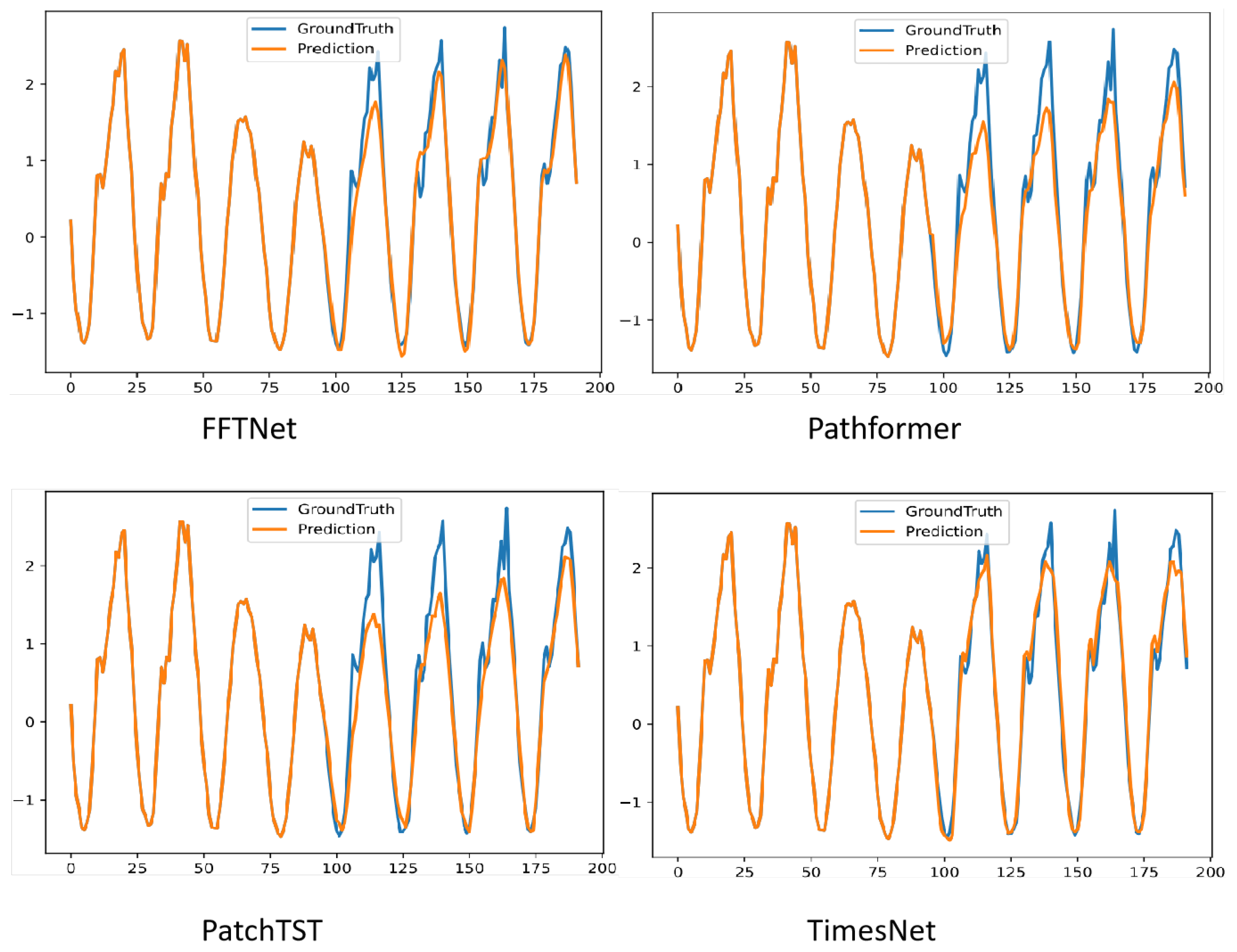
Figure 4 illustrates the comparison of prediction outcomes between FFTNet and baseline approaches, specifically Pathformer, PatchTST, and TimesNet, on the Traffic dataset, exhibiting pronounced non-stationary features. FFTNet amalgamates the frequency enhancement attributes of the multi-layer perceptron (MLP) in the frequency domain with the spatio-temporal dynamic modelling capabilities of the two-dimensional convolutional neural network (CNN), resulting in a prediction curve that closely aligns with the ground truth.

Figure 4.
Visualisation on Traffic by different models under input-96-predict-96 settings.
Secondly, we displayed the prediction outcomes for the ETTm1, Weather, and ILI datasets, as illustrated in Figure 5. Notwithstanding considerable disparities in data patterns—exemplified by the pronounced daily/weekly periodicity of the Electricity data, the multi-variable coupled abrupt changes in the Weather data, and the elevated sparsity and non-stationary peaks of the ILI data—successful predictions can be attained through the synergistic approach of global pattern recognition in the frequency domain and local abrupt change detection in the time domain.

Figure 5.
Visualisation of forecasting results on multiple datasets by FFTNet.
To assess the model’s adaptability for long-sequence prediction, we evaluated the performance of FFTNet across several prediction windows [96, 192, 336, 720] on the ETTh1 dataset, as illustrated in Figure 6. The results demonstrate that for prediction windows of [96, 192, 336], the prediction curves of FFTNet continue to exhibit periodic phase synchronisation with the actual values. In the extensive long-range task of forecasting 720 steps using 96 historical steps as input, FFTNet exhibits a strong capacity to model trend fluctuations (gradually increasing power load) during the initial 400 steps. Near the 500th step, the actual value undergoes a precipitous decline, akin to the abrupt decrease in load due to a power grid failure, whereas the model’s prediction curve persists in following the historical growth trend, leading to a substantial divergence in the prediction trajectory from the 500th to the 720th step.
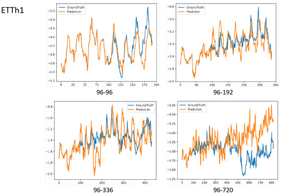
Figure 6.
Visualisation of forecasting results on ETTh1. The look-back length is 96.
Despite FFTNet’s exceptional performance in ordinary contexts via the integration of time and frequency domains, it encounters an adaptability limitation when faced with extreme sudden shifts beyond the training data distribution. The model may excessively depend on the statistical characteristics of the training data throughout the learning phase and lacks the capacity to effectively simulate unusual extreme scenarios.
4.6. Ablation Study
To assess the efficacy of LCCB and GCR components, we performed ablation experiments on many datasets by omitting either the LCCB or GCR. The findings are illustrated in Table 4. For each ablation experiment, we maintained the fundamental parameter values while sequentially removing one module, modifying the input dimension of the final linear layer to ensure proper model functionality. Longitudinal time series forecasting studies were conducted on five datasets, Weather, ETTh1, ETTh2, ETTm1, and ETTm2, with prediction horizons . The MSE and MAE scores were averaged across the four studies.
Table 4.
An ablation study examining the efficacy of LCCB and GCR within FFTNet. The terms Full, w/o LCCB, and w/o GCR denote the whole model, the model with the LCCB module omitted, and the model with the GCR module omitted, respectively. The MSE and MAE metrics represent the average values for prediction intervals . The optimal findings are emphasised in bold, whereas the suboptimal results are underlined.
In the five datasets and ten measures analysed, our fully integrated FFTNet secured first position in five metrics and second place in the other five. An in-depth examination of the results indicates that the elimination of the LCCB module from the Weather dataset leads to a substantial decline in performance, while the removal of the GCR module from the ETTh1 dataset produces a comparable effect. This illustrates the significance of utilising both frequency and temporal data for reliable forecasting. In instances when the complete-module FFTNet exhibited marginally inferior performance compared to its ablated counterparts, the decline in performance was negligible. The results unequivocally demonstrate that the fully integrated FFTNet routinely surpasses systems utilising either the LCCB or GCR module.
We executed a number of studies to thoroughly ascertain the ideal patch size and stride. To this end, we employed several prevalent combinations, namely [64,32], [32,16], [16,8], [8,8], [16,16], and [16,32]. These combinations were carefully selected to comprehensively explore different data partitioning strategies, aiming to find the most effective configuration for time series prediction.
The experiments were conducted across various datasets, including ETTh1, ETTh2, ETTm1, ETTm2, and the Weather dataset. We used two key evaluation metrics, Mean Squared Error (MSE) and Mean Absolute Error (MAE), to assess the performance of each combination. MSE measures the average of the squares of the errors, which emphasises larger errors, while MAE measures the average of the absolute errors, providing a more straightforward indication of the average error magnitude.
From a theoretical perspective, the choice of patch size and stride is closely related to important concepts in signal processing. According to Shannon’s sampling theorem, to recover the original signal without distortion from the sampled signal, the sampling frequency must be greater than or equal to twice the highest frequency of the original signal. In the context of time series processing, appropriate patch size and stride can “sample” the time series at a proper frequency, thereby capturing the key information and variation patterns in the data. If the stride is too large, it may result in an excessively low sampling frequency and cause the loss of important high-frequency information. If the stride is too small, it will increase the computational load and may introduce excessive redundant information.
The findings, illustrated in Table 5, demonstrate that a patch size of 16 and a stride of 8 yielded optimal performance. This combination was able to strike a good balance between capturing local features (due to the appropriate patch size) and efficiently processing the data (due to the suitable stride). It showed consistent and superior performance across multiple datasets, indicating its robustness and adaptability in different time series prediction scenarios. Therefore, we conclude that the [16,8] combination is the most suitable choice for our time series prediction task.
Table 5.
Ablation study on patch size and stride.
4.7. Model Analysis
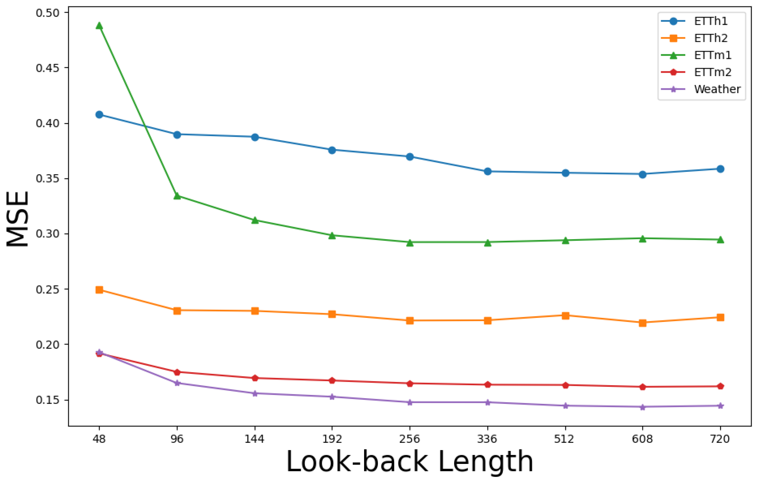
An effective long-term time series forecasting (LTSF) model typically yields more accurate predictions with an extended lookback window, as supplementary collected data enable the algorithm to identify additional trends and periodic patterns. Nonetheless, an extended duration of collected data also elevates the model’s complexity. Numerous Transformer-based models have difficulties when handling large time series data that surpass 96 time steps [20].
Figure 7 illustrates that FFTNet’s performance shows a reduction or stability in prediction error as the lookback window increases, underscoring its adaptability and durability across different window lengths. This stability enables FFTNet to provide dependable predictive outcomes across various lookback window sizes.
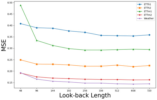
Figure 7.
Prediction error of FFTNet utilising various lookback windows, with a prediction length fixed at 96.
As illustrated in Table 6, FFTNet markedly surpasses other Transformer-based models regarding parameter count and multiply–accumulate operations (MACs). NLinear [8] utilises a channel-wise independent single linear layer, leading to markedly reduced parameter counts, multiply–accumulate operations (MACs), and training duration per epoch in comparison to alternative methods. Although it has the best efficiency of the compared models, its prediction performance is not competitive with the transformer-based methods. FFTNet significantly decreases model size and processing requirements while preserving reasonably rapid training speeds, hence offering a distinct efficiency advantage. This improvement reduces model complexity and resource consumption, while increasing scalability and practical applicability in real-world situations. Specifically, in contexts requiring extensive datasets or real-time forecasting, FFTNet’s streamlined architecture renders it an ideal selection.
Table 6.
Comparison of the efficiency of FFTNet and other models on the electricity dataset, utilising a lookback window of and a prediction length of .
4.8. Robustness Analysis
We incorporated Gaussian noise into various datasets to replicate typical real-world noise disturbances and assess the robustness of our methodology. Gaussian noise with a variance of 0.2 times the original variance of the input sequence was incorporated into the data. The model was trained on noise-injected datasets, and its performance was assessed using Mean Squared Error (MSE) and Mean Absolute Error (MAE), as shown in Table 7.
Table 7.
Performance metrics of noisy time series data.
The experimental results demonstrate that, notwithstanding the introduced noise, our technique displayed only a marginal reduction in these critical parameters. This illustrates the method’s resilience to input noise, allowing it to withstand interference and sustain consistent predicted performance. Table 6 further illustrates that, despite the presence of noise, the model continually achieves low error rates, showcasing exceptional predictive accuracy and stability.
5. Conclusions
This study focuses on long-term time series forecasting and introduces FFTNet, a novel hybrid model. FFTNet integrates the Local-Context ConvBlock (LCCB) and the Global-Cyclic Recogniser (GCR) to effectively capture both local and global patterns in time series data, hence improving prediction accuracy. The patching methodology was implemented for the analysis of input time series. Theoretical investigation, utilising Takens’ theorem, demonstrated that the patching method has significant correlations with phase space reconstruction in time series and is equal in phase space representation under certain conditions.
A comparison was conducted between the components of 2D CNNs and 1D CNNs. The 2D CNNs, utilising tensors derived from patching processes, function along inter-patch and intra-patch dimensions. This bypasses the convoluted feature learning in one-dimensional operations and facilitates hierarchical feature extraction using single-layer kernels. Parseval’s Theorem and the Convolution Theorem were employed for the analysis of the frequency multilayer perceptron (Frequency MLP) and the time-domain multilayer perceptron (Time-domain MLP). The Frequency MLP may modify the signal spectrum in the frequency domain, efficiently decoupling multi-scale components in time series forecasting. Conversely, the Time-domain MLP directly converts the original time-domain signal and exhibits difficulties in managing non-stationary time series. Comprehensive trials on real-world datasets revealed FFTNet’s exceptional performance in Mean Squared Error (MSE) and Mean Absolute Error (MAE), its ability to capture time series dynamics, and improved computing efficiency. Ablation experiments further confirmed the importance of the LCCB and GCR modules, substantiating the model’s architecture.
6. Limitations and Future Work
Although FFTNet demonstrates remarkable efficacy in typical scenarios by merging the time and frequency domains, it exhibits limitations in adaptability when faced with extreme and abrupt changes that exceed the training data distribution. During the training phase, the model may excessively depend on the statistical properties of the training data and lack the capacity to accurately replicate atypical severe circumstances.
To address this issue, future research may investigate the implementation of more robust anomaly detection mechanisms or the utilisation of techniques such as generative adversarial networks (GANs) to enhance the model’s adaptability in challenging conditions, while also considering the attention mechanism. By dynamically allocating weights, it may integrate time-domain and frequency-domain elements more flexibly and intelligently, hence augmenting the model’s capacity to discern intricate data patterns and strengthening its performance under extreme conditions.
Author Contributions
Conceptualisation, Z.Y.; methodology, Z.Y.; software, Z.Y.; validation, Z.Y. and J.L. (Junjie Liao); resources, M.Y. and B.H.; writing—original draft, Z.Y.; writing—review and editing, M.Y.; visualisation, Z.Y., J.L. (Jiachao Li) and F.X.; supervision, M.Y., P.Z. and B.H.; project administration, Z.Y. All authors have read and agreed to the published version of the manuscript.
Funding
Our research was supported by the Guangxi Natural Science Foundation (Grant NO. 2025GXNSFAA069359).
Data Availability Statement
The data that support the findings of this study are available in FFTNet at https://github.com/mackery/FFTNet.git, accessed on 23 March 2025. These data were derived from the following resources available in the public domain: ETTh, Weather, Traffic, and Electricity, https://drive.google.com/drive/folders/1ZOYpTUa82_jCcxIdTmyr0LXQfvaM9vIy, accessed on 23 March 2025.
Conflicts of Interest
The authors declare no conflicts of interest.
References
- Li, L.; Carver, R.; Lopez-Gomez, I.; Sha, F.; Anderson, J. Generative emulation of weather forecast ensembles with diffusion models. Sci. Adv. 2024, 10, eadk4489. [Google Scholar] [CrossRef] [PubMed]
- Zheng, X.; Shao, H.; Yan, S.; Xiao, Y.; Liu, B. Multiscale information enhanced spatial-temporal graph convolutional network for multivariate traffic flow forecasting via magnifying perceptual scope. Eng. Appl. Artif. Intell. 2024, 136, 109010. [Google Scholar] [CrossRef]
- Edalatpanah, S.A.; Hassani, F.S.; Smarandache, F.; Sorourkhah, A.; Pamucar, D.; Cui, B. A hybrid time series forecasting method based on neutrosophic logic with applications in financial issues. Eng. Appl. Artif. Intell. 2024, 129, 107531. [Google Scholar] [CrossRef]
- Yang, C.; Yan, J.; Wang, G. Time Series Trends Forecasting for Manufacturing Enterprises in the Digital Age. J. Organ. End User Comput. (JOEUC) 2024, 36, 1–22. [Google Scholar] [CrossRef]
- Wen, Q.; Zhou, T.; Zhang, C.; Chen, W.; Ma, Z.; Yan, J.; Sun, L. Transformers in time series: A survey. arXiv 2022, arXiv:2202.07125. [Google Scholar]
- Wang, H.; Peng, J.; Huang, F.; Wang, J.; Chen, J.; Xiao, Y. Micn: Multi-scale local and global context modeling for long-term series forecasting. In Proceedings of the Eleventh International Conference on Learning Representations, Kigali, Rwanda, 1–5 May 2023. [Google Scholar]
- Wu, H.; Hu, T.; Liu, Y.; Zhou, H.; Wang, J.; Long, M. Timesnet: Temporal 2d-variation modeling for general time series analysis. arXiv 2022, arXiv:2210.02186. [Google Scholar]
- Ailing, Z.; Muxi, C.; Lei, Z.; Qiang, X. Are transformers effective for time series forecasting. In Proceedings of the AAAI conference on artificial intelligence, Washington, DC, USA, 7–14 February 2023. [Google Scholar]
- Chen, S.A.; Li, C.L.; Yoder, N.; Arik, S.O.; Pfister, T. Tsmixer: An all-mlp architecture for time series forecasting. arXiv 2023, arXiv:2303.06053. [Google Scholar]
- Yi, K.; Zhang, Q.; Fan, W.; Wang, S.; Wang, P.; He, H.; An, N.; Lian, D.; Cao, L.; Niu, Z. Frequency-domain MLPs are more effective learners in time series forecasting. Adv. Neural Inf. Process. Syst. 2024, 36, 76656–76679. [Google Scholar]
- Lin, S.; Lin, W.; Wu, W.; Zhao, F.; Mo, R.; Zhang, H. SegRNN: Segment Recurrent Neural Network for Long-Term Time Series Forecasting. arXiv 2023, arXiv:2308.11200. [Google Scholar]
- Wen, R.; Torkkola, K.; Narayanaswamy, B.; Madeka, D. A multi-horizon quantile recurrent forecaster. arXiv 2017, arXiv:1711.11053. [Google Scholar]
- Liu, S.; Yu, H.; Liao, C.; Li, J.; Lin, W.; Liu, A.X.; Dustdar, S. Pyraformer: Low-complexity pyramidal attention for long-range time series modeling and forecasting. In Proceedings of the International Conference on Learning Representations, Vienna, Austria, 4 May 2021. [Google Scholar]
- Zhang, Y.; Ma, L.; Pal, S.; Zhang, Y.; Coates, M. Multi-resolution Time-Series Transformer for Long-term Forecasting. In Proceedings of the International Conference on Artificial Intelligence and Statistics, PMLR, Valencia, Spain, 2–4 May 2024; pp. 4222–4230. [Google Scholar]
- Whittle, P. Prediction and Regulation by Linear Least-Square Methods; Mathematical Control Theory; English University Press: London, UK, 1963. [Google Scholar]
- Atesongun, A.; Gulsen, M. A Hybrid Forecasting Structure Based on Arima and Artificial Neural Network Models. Appl. Sci. 2024, 14, 7122. [Google Scholar] [CrossRef]
- Li, S.; Jin, X.; Xuan, Y.; Zhou, X.; Chen, W.; Wang, Y.X.; Yan, X. Enhancing the Locality and Breaking the Memory Bottleneck of Transformer on Time Series Forecasting. In Proceedings of the Advances in Neural Information Processing Systems; Wallach, H., Larochelle, H., Beygelzimer, A., d’Alché-Buc, F., Fox, E., Garnett, R., Eds.; Curran Associates, Inc.: San Francisco, CA, USA, 2019; Volume 32. [Google Scholar]
- Zhou, H.; Zhang, S.; Peng, J.; Zhang, S.; Li, J.; Xiong, H.; Zhang, W. Informer: Beyond Efficient Transformer for Long Sequence Time-Series Forecasting. arXiv 2020, arXiv:2012.07436. [Google Scholar] [CrossRef]
- Wu, H.; Xu, J.; Wang, J.; Long, M. Autoformer: Decomposition Transformers with Auto-Correlation for Long-Term Series Forecasting. In Proceedings of the Neural Information Processing Systems, Online, 6–14 December 2021. [Google Scholar]
- Nie, Y.; Nguyen, N.H.; Sinthong, P.; Kalagnanam, J. A time series is worth 64 words: Long-term forecasting with transformers. arXiv 2022, arXiv:2211.14730. [Google Scholar]
- Lai, G.; Chang, W.C.; Yang, Y.; Liu, H. Modeling Long- and Short-Term Temporal Patterns with Deep Neural Networks. In Proceedings of the 41st International ACM SIGIR Conference on Research & Development in Information Retrieval, New York, NY, USA, 8–12 July 2018; SIGIR ’18. pp. 95–104. [Google Scholar] [CrossRef]
- Bergsma, S.; Zeyl, T.; Rahimipour Anaraki, J.; Guo, L. C2FAR: Coarse-to-Fine Autoregressive Networks for Precise Probabilistic Forecasting. In Proceedings of the Advances in Neural Information Processing Systems; Koyejo, S., Mohamed, S., Agarwal, A., Belgrave, D., Cho, K., Oh, A., Eds.; Curran Associates, Inc.: San Francisco, CA, USA, 2022; Volume 35, pp. 21900–21915. [Google Scholar]
- Tan, Y.; Xie, L.; Cheng, X. Neural Differential Recurrent Neural Network with Adaptive Time Steps. arXiv 2023, arXiv:2306.01674. [Google Scholar] [CrossRef]
- Fan, W.; Zheng, S.; Yi, X.; Cao, W.; Fu, Y.; Bian, J.; Liu, T.Y. DEPTS: Deep Expansion Learning for Periodic Time Series Forecasting. arXiv 2022, arXiv:2203.07681. [Google Scholar]
- Wang, S.; Wu, H.; Shi, X.; Hu, T.; Luo, H.; Ma, L.; Zhang, J.Y.; Zhou, J. Timemixer: Decomposable multiscale mixing for time series forecasting. arXiv 2024, arXiv:2405.14616. [Google Scholar]
- Li, Z.; Rao, Z.; Pan, L.; Xu, Z. MTS-Mixers: Multivariate Time Series Forecasting via Factorized Temporal and Channel Mixing. arXiv 2023, arXiv:2302.04501. [Google Scholar]
- Das, A.; Kong, W.; Leach, A.B.; Mathur, S.; Sen, R.; Yu, R. Long-term Forecasting with TiDE: Time-series Dense Encoder. arXiv 2023, arXiv:2304.08424. [Google Scholar]
- Liu, M.; Zeng, A.; Chen, M.; Xu, Z.; Lai, Q.; Ma, L.; Xu, Q. Scinet: Time series modeling and forecasting with sample convolution and interaction. Adv. Neural Inf. Process. Syst. 2022, 35, 5816–5828. [Google Scholar]
- Cao, D.; Wang, Y.; Duan, J.; Zhang, C.; Zhu, X.; Huang, C.; Tong, Y.; Xu, B.; Bai, J.; Tong, J.; et al. Spectral temporal graph neural network for multivariate time-series forecasting. Adv. Neural Inf. Process. Syst. 2020, 33, 17766–17778. [Google Scholar]
- Zhang, L.; Aggarwal, C.; Qi, G.J. Stock price prediction via discovering multi-frequency trading patterns. In Proceedings of the 23rd ACM SIGKDD International Conference on Knowledge Discovery and Data Mining, Halifax, NS, Canada, 13–17 August 2017; pp. 2141–2149. [Google Scholar]
- Woo, G.; Liu, C.; Sahoo, D.; Kumar, A.; Hoi, S. Cost: Contrastive learning of disentangled seasonal-trend representations for time series forecasting. arXiv 2022, arXiv:2202.01575. [Google Scholar]
- Zhou, T.; Ma, Z.; Wen, Q.; Sun, L.; Yao, T.; Yin, W.; Jin, R. Film: Frequency improved legendre memory model for long-term time series forecasting. Adv. Neural Inf. Process. Syst. 2022, 35, 12677–12690. [Google Scholar]
- Xu, Z.; Zeng, A.; Xu, Q. FITS: Modeling time series with 10k parameters. arXiv 2023, arXiv:2307.03756. [Google Scholar]
- Moosavi, V.; Vafakhah, M.; Shirmohammadi, B.; Behnia, N. A wavelet-ANFIS hybrid model for groundwater level forecasting for different prediction periods. Water Resour. Manag. 2013, 27, 1301–1321. [Google Scholar] [CrossRef]
- Joo, T.W.; Kim, S.B. Time series forecasting based on wavelet filtering. Expert Syst. Appl. 2015, 42, 3868–3874. [Google Scholar] [CrossRef]
- Oreshkin, B.N.; Carpov, D.; Chapados, N.; Bengio, Y. N-BEATS: Neural basis expansion analysis for interpretable time series forecasting. arXiv 2019, arXiv:1905.10437. [Google Scholar]
- Yang, Z.; Yan, W.; Huang, X.; Mei, L. Adaptive Temporal-Frequency Network for Time-Series Forecasting. IEEE Trans. Knowl. Data Eng. 2022, 34, 1576–1587. [Google Scholar] [CrossRef]
- Zhou, T.; Ma, Z.; Wen, Q.; Wang, X.; Sun, L.; Jin, R. Fedformer: Frequency enhanced decomposed transformer for long-term series forecasting. In Proceedings of the International Conference on Machine Learning, PMLR, Baltimore, MD, USA, 17–23 July 2022; pp. 27268–27286. [Google Scholar]
- Dai, T.; Wu, B.; Liu, P.; Li, N.; Bao, J.; Jiang, Y.; Xia, S.T. Periodicity decoupling framework for long-term series forecasting. In Proceedings of the Twelfth International Conference on Learning Representations, Vienna, Austria, 7–11 May 2024. [Google Scholar]
- Chen, P.; Zhang, Y.; Cheng, Y.; Shu, Y.; Wang, Y.; Wen, Q.; Yang, B.; Guo, C. Pathformer: Multi-scale transformers with adaptive pathways for time series forecasting. arXiv 2024, arXiv:2402.05956. [Google Scholar]
- Takens, F. Detecting strange attractors in turbulence. In Dynamical Systems and Turbulence, Warwick 1980; Rand, D., Young, L.S., Eds.; Springer: Berlin/Heidelberg, Germany, 1981; pp. 366–381. [Google Scholar]
- Yi, K.; Fei, J.; Zhang, Q.; He, H.; Hao, S.; Lian, D.; Fan, W. FilterNet: Harnessing Frequency Filters for Time Series Forecasting. In Proceedings of the Thirty-eighth Annual Conference on Neural Information Processing Systems, Vancouver, BC, Canada, 10–15 December 2024. [Google Scholar]
- Ma, X.; Li, X.; Fang, L.; Zhao, T.; Zhang, C. U-Mixer: An Unet-Mixer Architecture with Stationarity Correction for Time Series Forecasting. In Proceedings of the AAAI Conference on Artificial Intelligence, Vancouver, BC, Canada, 20–27 February 2024; Volume 38, pp. 14255–14262. [Google Scholar]
- Loshchilov, I.; Hutter, F. Fixing weight decay regularization in adam. arXiv 2017, arXiv:1711.05101. [Google Scholar]
- Liu, Y.; Hu, T.; Zhang, H.; Wu, H.; Wang, S.; Ma, L.; Long, M. itransformer: Inverted transformers are effective for time series forecasting. arXiv 2023, arXiv:2310.06625. [Google Scholar]


Disclaimer/Publisher’s Note: The statements, opinions and data contained in all publications are solely those of the individual author(s) and contributor(s) and not of MDPI and/or the editor(s). MDPI and/or the editor(s) disclaim responsibility for any injury to people or property resulting from any ideas, methods, instructions or products referred to in the content. |
© 2025 by the authors. Licensee MDPI, Basel, Switzerland. This article is an open access article distributed under the terms and conditions of the Creative Commons Attribution (CC BY) license (https://creativecommons.org/licenses/by/4.0/).