Dual-Task Learning for Long-Range Classification in Single-Pixel Imaging Under Atmospheric Turbulence

Abstract

Unlike traditional imaging, single-pixel imaging (SPI) exhibits greater resistance to atmospheric turbulence. Therefore, we use SPI for long-range classification, in which atmospheric turbulence often cause significant degradation in performance. We propose a dual-task learning method for SPI classification. Specifically, we design the Long-Range Dual-Task Single-Pixel Network (LR-DTSPNet) to perform object classification and image restoration simultaneously, enhancing the model’s generalization and robustness. Attention mechanisms and residual convolutions are used to strengthen feature modeling and improve classification performance on low-resolution images. To improve the efficiency of SPI, low-resolution objects are used in this work. Experimental results on the DOTA remote sensing dataset demonstrate that our method significantly outperforms conventional object classification approaches. Furthermore, our approach holds promise for delivering high-quality images that are applicable to other computer vision tasks.

1. Introduction

Object classification, as one of the fundamental computer vision tasks, has extensive applications in military, medical, industrial, and other fields [1,2,3,4]. However, in applications such as airborne and ground-based remote sensing, atmospheric turbulence induces image distortion and speckle noise in optical imaging systems, thereby severely compromising the classification accuracy of remote sensing data. Although deep-learning-based approaches have demonstrated efficacy in complex imaging or detection scenarios such as rainy weather and underwater environments [5,6,7], SPI exhibits unique advantages in long-range imaging or classification applications, particularly in remote sensing domains that require photon-efficient detection or atmospheric penetration capabilities [8,9,10]. Wang et al. proposed a physics-enhanced SPI neural network, achieving single-pixel LiDAR imaging at an outdoor distance of 570 m [8]. Li et al. proposed an SPI reconstruction method based on an untrained convolutional autoencoder network (UCAN), achieving high-quality long-range SPI in real urban atmospheric environments [9]. In addition to remote sensing applications, SPI has also been demonstrated to work in other complex imaging conditions [11,12,13,14,15,16,17]. Li et al. proposed a single-pixel object inspection system based on the compressive sensing super-resolution convolutional neural network (CS-SRCNN), which achieves high imaging quality in low-light and complex underwater environments [13]. He et al. proposed an SPI method based on the random discarding mechanism that simulates light scattering loss and system noise in complex environments through random discarding. This approach effectively suppresses interference under challenging imaging conditions [14]. Deng et al. projected structured patterns through a flame on an occluded scene and used the high dynamic range and high sensitivity of a single-pixel detector to capture backscattered signals, achieving full-color real-time imaging through the flame [16]. Zhang et al. achieved high-resolution microscopic imaging through complex scattering media by integrating temporal corrections with single-pixel microscopic imaging [17]. Evidently, SPI has significant application potential in various complex environments due to its advantages, including a broad spectral range, high sensitivity, simple structure, and strong anti-interference capability.

SPI requires two optical paths: a reference path and a signal path. Later, the reference path is emulated using a computer. The light in the signal path is modulated by a digital micromirror device (DMD) pattern, allowing it to interact with the object and then to be collected by a single-pixel detector as one-dimensional measurements. Reconstructed images are obtained by calculating these measurements with the corresponding modulation patterns. This approach of using a DMD or spatial light modulator (SLM) to replace the reference path was proposed by Shapiro in 2008, marking a fundamental development in SPI [18].

Although SPI has strong resistance to turbulence, the quality of reconstruction still needs to be improved. To mitigate the effect of turbulence, researchers primarily focus on two areas: the imaging system and the reconstruction algorithms. In terms of imaging systems, Fu et al. demonstrated that the result of imaging through turbulence is a superposition of turbulence-correlated and target-correlated results. Therefore, by isolating and subtracting the component correlated with turbulence, their method achieved great turbulence mitigation [19]. Wang et al. addressed the issue from the perspective of the light source, substituting the conventional Gaussian light source with a four-petal Gaussian source, which significantly enhanced the image quality in long-range imaging through atmospheric turbulence [20]. In terms of imaging algorithms, rapid advances in deep learning have enabled numerous teams to apply neural networks to counteract the effects of turbulence on SPI. Zhang et al. simulated atmospheric turbulence using phase screens and combined a Fourier filter with a conditional generative adversarial network (cGAN) to achieve a peak signal-to-noise ratio (PSNR) of 20 dB and a structural similarity index (SSIM) above 0.6 for reconstructed images [21]. Wang et al. proposed a physics-enhanced deep learning approach that incorporates the forward physical priors of SPI, enabling effective outdoor imaging for single-pixel radar systems [8]. Moreover, Zhang et al. utilized a multiscale GAN (MsGAN) to enhance image clarity [22]. Furthermore, Zhang et al. reshaped 1D SPI measurements into a 2D data frame as input to a GAN to effectively mitigate turbulence [23]. Cheng et al. combined the multiple-input–multiple-output (MIMO) and channel attention mechanism, significantly eliminating the effects of atmospheric turbulence [24].

In the field of object classification, SPI-based methods can be categorized into two approaches: image-based classification and image-free classification. Image-based classification involves first reconstructing images using traditional or deep learning algorithms, which are then fed into end-to-end image classification algorithms. Wang et al. proposed a single-stage end-to-end network trained on simulated data to achieve image reconstruction without modulation patterns, achieving 92% classification accuracy on the MNIST handwritten dataset with a sampling rate of 6.25% [25]. In contrast, image-free classification simplifies the process by directly feeding 1D measurements into classification algorithms [26]. Li et al. incorporated measurement values and Hadamard modulation patterns into the image classification network, further reducing object classification time and improving classification accuracy, thus demonstrating the optimization of computational ghost imaging systems through deep learning techniques [27]. Zhang et al. ingeniously utilized the convolutional neural network to optimize modulation patterns, achieving the real-time classification of fast moving targets [28]. Yang et al. proposed a multitask learning method (SP-ILC) capable of performing image reconstruction, object classification, and localization simultaneously [29]. Peng et al. developed a low-sampling-rate, non-imaging target detection method based on the Transformer architecture [30].

Although many SPI-based object classification methods have been developed, few focus on long-range SPI object classification under atmospheric turbulence, particularly for low-resolution objects which are common in long-range classification. In this work, we focus on $32\times 32$ low-resolution images affected by atmospheric turbulence. Although there have been many deep classification networks, they did not work well in our initial study on this task. We notice that the quality of the reconstructed images in SPI is very important for classification performance. Thus, in this work, we adopt a dual-task learning approach, in which object classification and image enhancement share a common backbone network. Additionally, the backbone integrates Swin–Conv Blocks within a UNet structure to enhance its modeling capability for low-resolution images, improving SPI imaging quality and classification accuracy. Our experimental findings indicate that our approach surpasses other end-to-end object classification networks in performance.

2. Theory

2.1. SPI for Atmospheric Turbulence

Atmospheric turbulence can be simulated using turbulence phase screens generated by power spectrum inversion, which has shown improved performance over alternative methods [31,32]. In the method, the atmospheric disturbance phase $\phi (x,y)$ can be defined as

$$\phi \left(x,y\right)=\mathbf{H}\left(x,y\right)exp\left\{i·{\mathcal{F}}^{-1}\left[\sqrt{PSD\left(f_x,f_y\right)}\Delta f\right]\right\},$$

(1)

where $\mathbf{H}$ is a complex Gaussian random matrix with zero mean and unit variance. The coordinates x and y specify positions in the spatial domain. Furthermore, i denotes the imaginary unit. ${\mathcal{F}}^{-1}\{·\}$ denotes the inverse Fourier transform. The symbol “·” denotes multiplication. The values $f_x$ and $f_y$ are the coordinates in the frequency domain. $\Delta f$ is the unit frequency spacing. In the equation, the power spectral density ($PSD$) of atmospheric turbulence is defined by Equation (2),

$$PSD\left(f_x,f_y\right)=PSD\left(k\right)=0.023r_0^{-5/3}{\displaystyle \frac{exp\left[-{\left(k/k_i\right)}^2\right]}{{\left(k^2+k_o^2\right)}^{11/6}}},$$

(2)

$$k=\sqrt{f_x^2+f_y^2},$$

(3)

where $r_0$ determines the strength of atmospheric turbulence. The parameters $k_i$ and $k_o$ represent the frequencies of the inner and outer scales of the turbulence, respectively, which determine the minimum and maximum turbulence. Utilizing the simulated phase plate $\phi \left(x,y\right)$ to an image, we have the degraded image with atmospheric turbulence effects.

In SPI, a source light is modulated by a DMD. Then the modulated light illuminates an object and is reflected to a single-pixel detector. In the light path, atmospheric turbulence happens to degrade the system performance. To reconstruct the object, a correlation calculation is performed between the 1D measurements collected by the single-pixel detector and the 2D modulation patterns displayed on the DMD. Note that, to achieve higher image resolution, generally, it requires a greater number of measurements. This is time-consuming. More importantly, in long-range detection, the objects usually have small sizes. Thus, in this work, we use low-resolution objects with a size of $(32\times 32)$.

For the reconstruction algorithm, we employ differential ghost imaging (DGI) [33] and total variation ghost imaging (TVGI) [34,35] for correlation-based reconstruction. DGI is based on ghost imaging (GI), where the bucket signal $B_n$ is replaced with the differential bucket signal $D_n$ to elevate the sensitivity of GI. The equations for ghost imaging and differential bucket signal are as follows:

$$G_{GI}\left(x,y\right)=〈\left(B_n-〈B_n〉\right)\left[I_n\left(x,y\right)-〈I_n\left(x,y\right)〉\right]〉,$$

(4)

$$D_n=B_n-{\displaystyle \frac{〈B_n〉}{〈R_n〉}}{R}_n,$$

(5)

where $B_n$ represents the intensity of the bucket signal, $R_n$ represents the total intensity of the modulation pattern, $I_n(x,y)$ indicates the spatial distribution of the modulation pattern, and $〈·〉$ represents the averaging operation. By replacing the bucket signal $B_n$ with the differential bucket signal $D_n$, we obtain the following equation for differential ghost imaging:

$$G_{DGI}\left(x,y\right)=〈B_n{I}_n\left(x,y\right)〉-{\displaystyle \frac{〈B_n〉}{〈R_n〉}}〈R_n{I}_n\left(x,y\right)〉.$$

(6)

In addition to DGI, we also employ the TVGI algorithm, which is basically a compressed sensing reconstruction algorithm used in SPI. This method incorporates total variation (TV) regularization as prior knowledge, allowing high-quality reconstructions at lower sampling rates. The Equations for the algorithm are as follows:

$$min\left[R_{TV}\left(O\right)\right]=\sum _{i=1}^N\left(\left|{\displaystyle \frac{d{I}_i\left(O\right)}{dx}}\right|+\left|{\displaystyle \frac{d{I}_i\left(O\right)}{dy}}\right|\right),$$

(7)

$$P\ast I\left(O\right)=B,$$

(8)

where $I_i\left(O\right)$ represents the 2D intensity of the reconstructed object, $R_{TV}\left(O\right)$ denotes the sum of the gradient magnitudes of $I_i\left(O\right)$, P is the modulation pattern, and B is the 1D measurement vector. The reconstruction process consists of iteratively solving the optimization problem defined by Equation (7), while simultaneously applying Equation (8) to assess image fidelity.

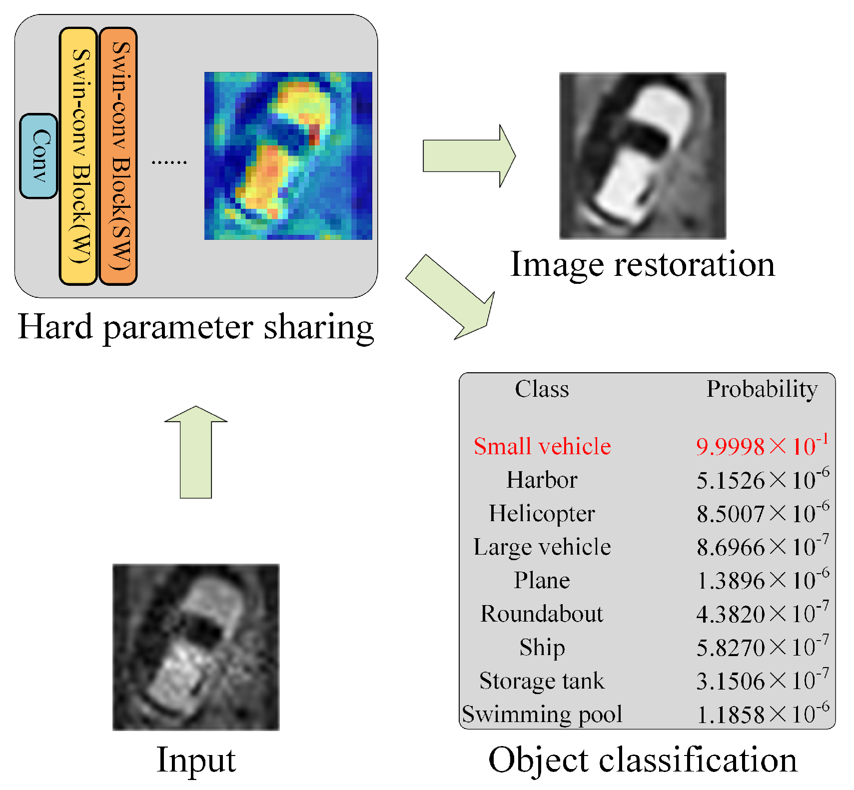
2.2. LR-DTSPNet for Dual-Task Learning

2.2.1. Dual-Task Learning

Based on the principle of dual-task learning [36], we employ a hard parameter sharing approach to jointly optimize the model parameter for two tasks, object classification and image restoration. The idea of our work is illustrated in Figure 1.

Dual-task learning can enhance a network’s ability to generalize because it shares backbone parameters and uses domain information from training signals for related tasks. In this work, dual-task learning improves object classification by using shared features between classification and image quality restoration. Both tasks require the extraction of high-level structural and textural information that is critical for accurate identification. By aligning these complementary tasks within a shared backbone, the network can develop a more nuanced representation of objects, leveraging restoration features to highlight key object contours and boundaries, and thus ultimately can enhance classification performance.

Furthermore, the image restoration task increases the robustness of the model by introducing a form of noise resilience. Because image quality enhancement inherently involves denoising and artifact removal, it enables the network to better handle noisy or degraded inputs, which are often encountered in long-range imaging. Consequently, this shared learning improves the stability and adaptability of the network in challenging visual environments, improving its generalization to diverse input conditions. The synergy between these tasks produces a model that is not only more accurate in object classification but also more resilient to visual distortions.

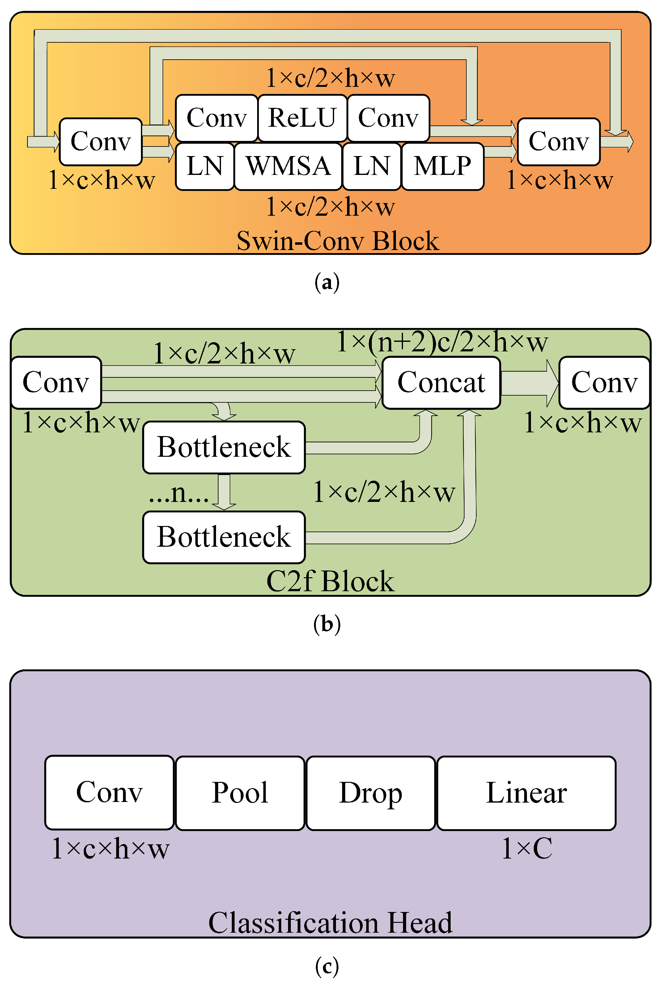
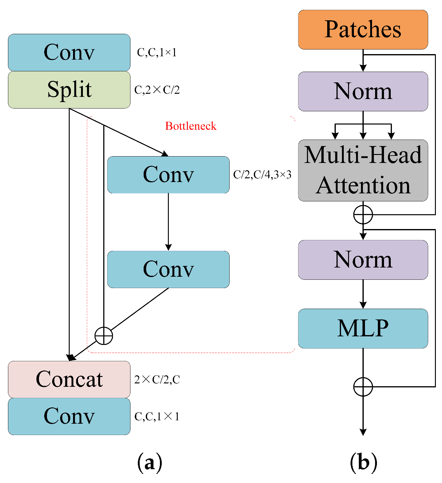
2.2.2. LR-DTSPNet Architecture

In this work, we focus on low-resolution objects that are common in long-range imaging. This makes the imaging speed of the SPI fast. However, object classification based on SPI reconstructions becomes a challenging task, especially under atmospheric turbulence. To address these challenges, we incorporate Swin–Conv Blocks into the network and adopt a dual-task learning approach to enhance the network’s classification performance.

The network consists of three main components: a backbone network, a classification network, and a restoration head. As illustrated in Figure 2, the backbone network has a UNet structure with three encoder modules and three decoder modules, enhanced with newly designed Swin–Conv Blocks [37] to improve the network’s ability to capture local and global feature information.

Using the architecture for our dual-task learning, firstly, a single-channel SPI reconstructed image is passed through the initial convolutional layer to increase its channel count to 32, and is then fed into the Swin–Conv Block in the first encoder. The architecture of the Swin–Conv Block is shown in Figure 3a. The Swin–Conv Block is composed of the convolutional residual path and the Swin Transformer path. Within each Swin–Conv Block, the input image is initially processed by a $1\times 1$ convolutional layer, then is split along the channel dimension into two parts. One part is sent to the convolutional residual path for local feature modeling, while the other is proceeded to the Swin Transformer path for global feature modeling. In the convolutional residual path, the input sequentially passes through a $3\times 3$ convolutional layer, a rectified linear unit ($ReLU$) activation layer, and another $3\times 3$ convolutional layer, before being combined with the input residual to produce the output. In the Swin Transformer path, the input sequentially passes through LayerNorm ($LN$) and window-based multi-head self-attention ($WMSA$), and is then combined with the input via a residual connection to obtain an intermediate representation. This intermediate representation is subsequently fed into $LN$ and a multilayer perceptron ($MLP$) layer, with the output of the $MLP$ being combined with the intermediate representation through a residual connection to produce the output of the Swin Transformer path. Finally, the outputs from both paths are concatenated along the channel dimension and subsequently passed through another $1\times 1$ convolutional layer to fuse the feature information, which is then combined with the input through a residual connection. The Swin–Conv Block is computed as Equation (9):

$$\begin{array}{c}\hfill x_c,x_t=Split\left(Conv\left(x_{in}^{sc}\right)\right),\\ \hfill {\widehat{x}}_c=Conv\left(ReLU\left(Conv\left(x_c\right)\right)\right)+x_c,\\ \hfill x_t^{\prime }=WMSA\left(LN\left(x_t\right)\right)+x_t,\\ \hfill {\widehat{x}}_t=MLP\left(LN\left(x_t^{\prime }\right)\right)+x_t^{\prime },\\ \hfill x_{out}^{sc}=Conv\left(Concat\left({\widehat{x}}_c,{\widehat{x}}_t\right)\right)+x_{in}^{sc},\end{array}$$

(9)

where $x_{in}^{sc}$ and $x_{out}^{sc}$ denote the input and output of the Swin–Conv Block, respectively. Similarly, $x_c$ and ${\widehat{x}}_c$ denote the input and output of the convolutional path, while $x_t$ and ${\widehat{x}}_t$ denote the input and output of the Swin Transformer path. Additionally, $x_t^{\prime }$ denotes the intermediate representation within the Swin Transformer path. The distinction between Swin–Conv Block (W) and Swin–Conv Block (SW) resides in their multi-head self-attention implementations. The former adopts $WMSA$, whereas the latter employs Shifted Window MSA ($SWMSA$) to facilitate inter-window information propagation, thereby enhancing the network’s capability to model global contextual dependencies [38]. The output of the Swin–Conv Block is then shrunk in size via a convolutional layer, preparing it for input into the next encoder. In the UNet architecture, skip connections are also used to maintain feature continuity across scales. For example, the input of Decoder 2 is the sum of the output of Encoder 2 and Decoder 3.

After extracting local and global features through the backbone network, the Decoder 1 output is fed simultaneously into both the classification network and the restoration head. The restoration head consists of a single $3\times 3$ convolutional layer. After this layer, the output of Decoder 1 with size of $1\times 32\times 32\times 32$ becomes a restored image with $1\times 1\times 32\times 32$. The classification network consists mainly of convolutional layers, C2f Blocks, and a Classification Head. The convolutional layers primarily adjust channel dimensions to accelerate computation efficiency. The C2f Blocks are responsible for extracting image features. The Classification Head generates label probabilities for each image, selecting the label with the highest probability as the classification result. The architectures of a C2f Block and the Classification Head are illustrated in Figure 3b,c. The C2f Block comprises convolutional layers and bottleneck units. Within each C2f Block, the input is first processed through a $1\times 1$ convolutional layer, then the output of the convolutional layer is divided along the channel dimension into two parts. A portion of the output remains unchanged, while the other portion is fed into a sequence of n bottleneck units. Within each bottleneck unit, the input undergoes a $3\times 3$ convolutional layer to reduce the channel count by half, followed by another $3\times 3$ convolutional layer to restore the original channel count. The final input of each bottleneck unit is obtained by adding the initial input to the output of the convolution operations. Finally, the outputs of each bottleneck unit, along with the two initial portions, totaling $n+2$ portions, are concatenated along the channel dimension. These concatenated features are then fused and their channel count is adjusted using a $1\times 1$ convolutional layer. The C2f Block and the bottleneck unit are computed as Equations (10) and (11).

$$\begin{array}{c}\hfill x_1,x_2=Split\left(Conv\left(x_{in}^{c2f}\right)\right),\\ \hfill x_3=Bottleneck\left(x_2\right),\\ \hfill x_{n+2}=Bottleneck\left(x_{n+1}\right),\\ \hfill x_{out}^{c2f}=Conv\left(Concat\left(x_1,x_2,\cdots ,x_{n+2}\right)\right),\end{array}$$

(10)

$$x_{out}^b=Conv\left(Conv\left(x_{in}^b\right)\right)+x_{in}^b,$$

(11)

where $x_{in}^{c2f}$ and $x_{out}^{c2f}$ denote the input and output of the C2f Block, respectively. $x_{in}^b$ and $x_{out}^b$ denote the input and output of the bottleneck unit. The number of bottlenecks configured for feature extraction in all three stages is set to [1, 2, 2]. Following three stages of feature extraction, the features are further processed through a series of convolutional, pooling, dropout, and fully connected layers to generate the final classification results.

2.2.3. Cost Function for LR-DTSPNet

Based on dual-task learning, object classification and image quality restoration tasks share the parameters of the backbone network, allowing for synchronized optimization through a combined loss function. In order to jointly supervise classification accuracy and restoration quality, we integrate the cross-entropy loss function for the classification task and the root mean squared error (RMSE) function for image quality evaluation into a unified loss function. The loss function of the cross-entropy is defined by Equation (12),

$$L_c=-p\left(I\right)log\left\{softmax\left[q\left(I\right)\right]\right\},$$

(12)

where I is the input image. $p\left(I\right)$ denotes the category label of the input image, represented as a one-hot vector, with the correct category set to 1 and all the others set to 0. Furthermore, $q\left(I\right)$ is the predicted classification probability. The RMSE to evaluate the image quality is defined as Equation (13).

$$L_r=\sqrt{{\displaystyle \frac{1}{h\times w}}\sum _{i=1}^{h\times w}{\left(y_i-{\widehat{y}}_i\right)}^2},$$

(13)

where h and w represent the height and width of the image, $y_i$ and ${\widehat{y}}_i$ are the intensities of the original and the restored images. Then, the total loss function of our method becomes

$$L={\lambda }_1{L}_c+{\lambda }_2{L}_r,$$

(14)

where ${\lambda }_1$ and ${\lambda }_2$ are two weights assigned to make the two loss components remaining in the same order of magnitude. The parameters ${\lambda }_1$ and ${\lambda }_2$ can be adjusted based on SPI quality. In this study, ${\lambda }_1$ and ${\lambda }_2$ were set to 1 and 0.01, respectively.

3. Simulation Experiments

3.1. Dataset

To verify the effectiveness of our method, we built various datasets based on different sampling rates and reconstruction schemes in SPI, as shown in Figure 4. The original objects for the experiments were all cropped from the DOTA remote sensing dataset [39]. Compared to other remote sensing datasets, the DOTA dataset offers a larger number of instances and more precise annotations, facilitating image cropping and network training. Therefore, we selected the DOTA dataset for our study. We cropped the images according to the instance bounding boxes provided in DOTA and resized them to a consistent dimension, resulting in the original images for SPI. The dataset contains a total of 201,407 images. The atmospheric turbulence was simulated by adding 100 layers of turbulent phase screens. The dataset includes images of swimming pools, ships, helicopters, storage tanks, small vehicles, roundabouts, harbors, planes, and large vehicles, totaling 201,407 images. The dataset is divided into training and validation sets in a ratio of 9:1. Single-pixel sampling processes were performed using Hadamard patterns and random grayscale patterns at sampling rates of 1.0, 0.5, 0.3, and 0.1, respectively. We utilized TV and DGI algorithms to reconstruct the objects for training and testing of a network.

Due to atmospheric turbulence, the details and textures of the reconstructed objects are generally severely deteriorated. Compared to the DGI method, the reconstructions using the TV method have better quality no matter whether it is Hadamard or random patterns for sampling. Between Hadamard and random patterns, when the TV method is used, the former present better reconstruction quality. Meanwhile, the image quality of each reconstruction scheme deteriorates rapidly as the sampling rate decreases, particularly for the DGI algorithm.

3.2. Object Classification

3.2.1. Recent Classification Network for Comparison

In our experiments, we selected several widely used object classification networks, including You Only Look Once (YOLO) [40], MobileNet [41], ConvNeXt [42], EfficientNet (EffNet) [43], Vision Transformer (ViT) [44], Swin Transformer (Swin) [38], and SP-ILC [29], for a comprehensive comparison.

Among the seven networks, the first four are based on CNN architectures. The YOLOv8 object classification network adopts the idea of Cross-Stage Partial Network (CSPNet), which splits the input into two parts within the backbone network [45]. One part is fed into the standard bottleneck structure, while the other remains unchanged and is directly concatenated with the bottleneck output along the channel dimension, as shown in Figure 5a. This structure not only reduces the parameter count and memory consumption, but also maintains or improves accuracy. As a representative lightweight network, MobileNetV3 decomposes the standard convolution into depth-wise convolution and $1\times 1$ point-wise convolution, effectively reducing computational cost and model size. Furthermore, ConvNeXt maintains the inherent simplicity and computational efficiency of convolutional networks while narrowing the performance gap with models based on transformer. Finally, the EffNetV2’s compound scaling method optimally balances network depth, width, and resolution, thereby achieving higher efficiency with fewer computational resources. It offers an optimal balance of precision and speed, which makes it particularly suitable for large-scale image recognition tasks.

With the advancement of attention mechanisms in recent years, the ViT based on attention mechanisms has attracted widespread attention. Inspired by transformers, the ViT network segments an input image into N patches, each of which is linearly mapped to a high-dimensional encoding. This encoded sequence is then fed into the transformer encoder, which consists of a multi-head attention module, a $MLP$, and normalization layers, as shown in Figure 5b. Initially, the encoded sequence undergoes normalization and subsequently splits into query, key, and value components for processing by the multi-head attention module. The module output is connected to the original input sequence via a residual connection and then processed through additional normalization and $MLP$ layers, finally producing the encoder output. ViT has the advantages of global modeling and parallel processing, achieving excellent performance in image classification tasks. Compared to ViT, the Swin shifted window mechanism facilitates local self-attention computation, significantly reducing computational complexity while preserving global context. This design not only increases scalability for high-resolution images, but also enhances performance in dense prediction tasks. For these reasons, we selected ViT and Swin for comparison.

The above six networks are image-based classification networks. For image-free classification, we selected the concurrent single-pixel imaging, object location, and classification method proposed by Yang et al. [29].

The experiment was carried out using YOLOv8s as the baseline and compared with ViT, Swin-T, ConvNeXt V2-T, EffNetV2-S, MobileNetV3, SP-ILC, and our proposed method. The model metrics for each network are shown in

Table 1. Model metrics of classification network.

Network	Parameter Count (M)	FLOPs (G)	Inference Speed (FPS)	Restoration
YOLOv8s	5	0.016	555	×
ViT	85	5.6	208	×
Swin-T	28	4.5	83	×
ConvNeXt V2-T	28.6	4.47	144	×
EffNetV2-S	21.5	8.4	100	×
MobileNetV3	4.2	0.0072	104	×
SP-ILC	2.3	0.12	225	√
Ours	4.1	0.17	48	√

. The inference speed was tested on a GPU with 24 GB of memory.

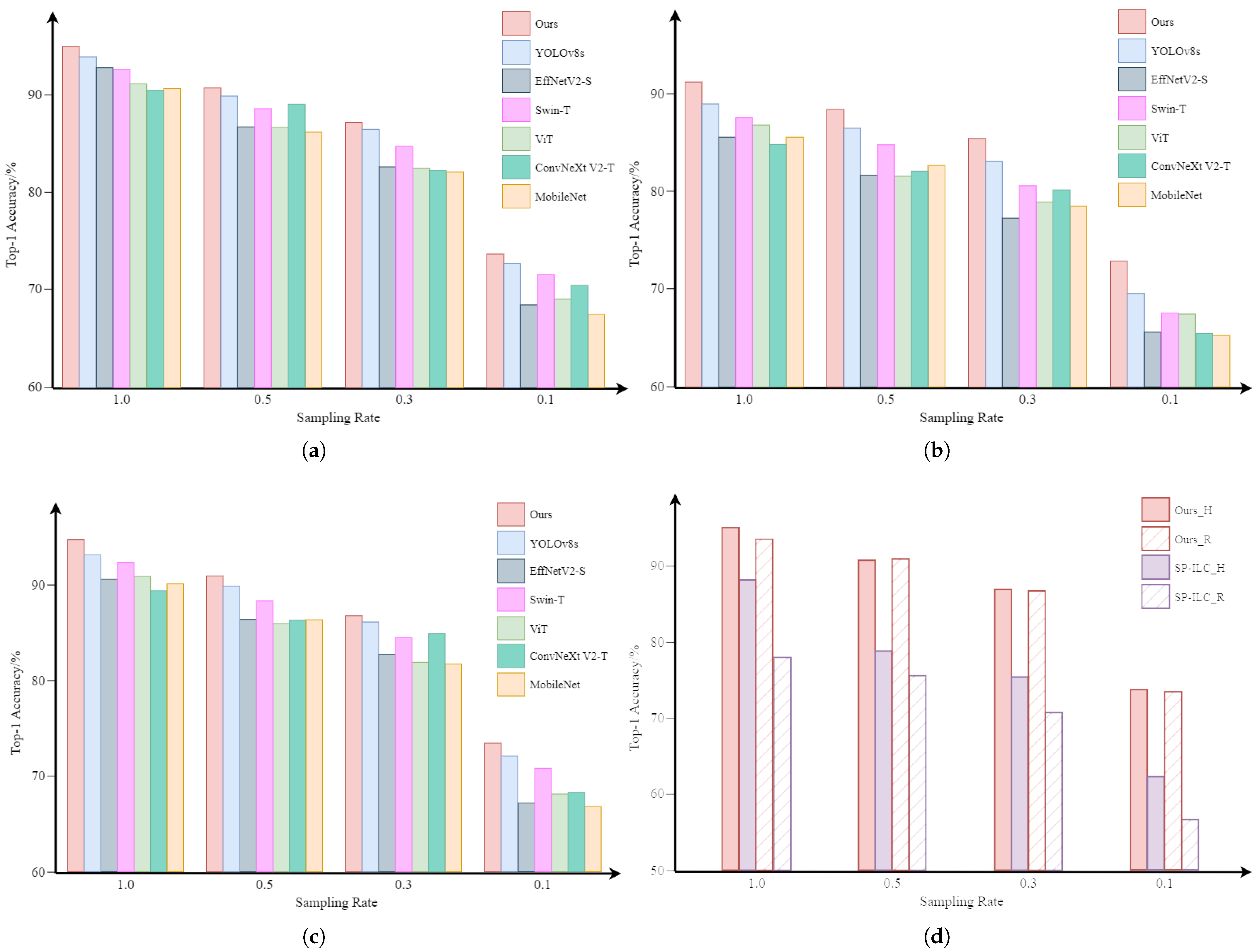
3.2.2. Classification Results

The hardware environment for the simulation experiments consists of a GPU with 24 GB of memory, and the operating system is Linux. The optimizer used for network training is AdamW, with an initial learning rate of $7\times {10}^{-4}$. The input image size is $32\times 32$, and the batch size is 256. Comparative experiments were carried out using PyTorch 2.0.1 with 400 training epochs, and the epochs with the highest classification accuracy were selected for comparison. The experimental results are illustrated in Figure 6. According to the experimental results, the method we proposed achieves the highest classification accuracy among all reconstruction scenarios, with a maximum accuracy of 95.08%. For different reconstruction schemes, on the TV_H dataset, our method improves accuracy by an average of 3.35%; on the TV_R dataset, the average improvement is 3.77%; and on the DGI_H dataset, the average improvement is 5.415%. For different sampling rates, with a full sampling rate of 1.0, our method improves accuracy by an average of 3.79%; at a sampling rate of 0.5, the average improvement is 3.94%; at a sampling rate of 0.3, the average improvement is 4.2%; and at a sampling rate of 0.1, the average improvement is 4.79%. It can be observed that experimental results demonstrate that our method consistently enhances classification accuracy under various degradation scenarios—whether stemming from different reconstruction scheme selection or sampling rate reduction. Furthermore, the greater the degradation of image quality, the more pronounced the improvement, indicating that the knowledge learned from the image quality restoration task contributes to improving classification performance. Furthermore, as shown in Figure 6a,b, our classification network consistently outperforms the baseline for different reconstruction algorithms. In particular, compared to the DGI_H case, our method achieves an average accuracy improvement of 3.1% compared to the baseline. Furthermore, Figure 6a,c demonstrate that our method exhibits the best classification performance in both Hadamard and random sampling patterns. Using the same TV reconstruction algorithm, our method achieved an average accuracy improvement of 0.8% with Hadamard patterns and 1.2% with random patterns, compared to the baseline. Lastly, Figure 6d illustrates that, compared to the image-free classification method, our method provides a substantial improvement in classification accuracy at different sampling rates and adapts to various measurement patterns. In particular, while achieving optimal performance, our network also reduces the parameter count by 18% compared to the baseline.

Figure 7 shows the attention maps generated by our method for different objects, indicating the robustness of the model to atmospheric turbulence and its ability to accurately focus on the target objects. The weight distribution in the attention maps reveals that the network effectively suppresses atmospheric turbulence while enhancing the features of the objects. This insight provides interpretability for the network’s ability to achieve optimal classification performance.

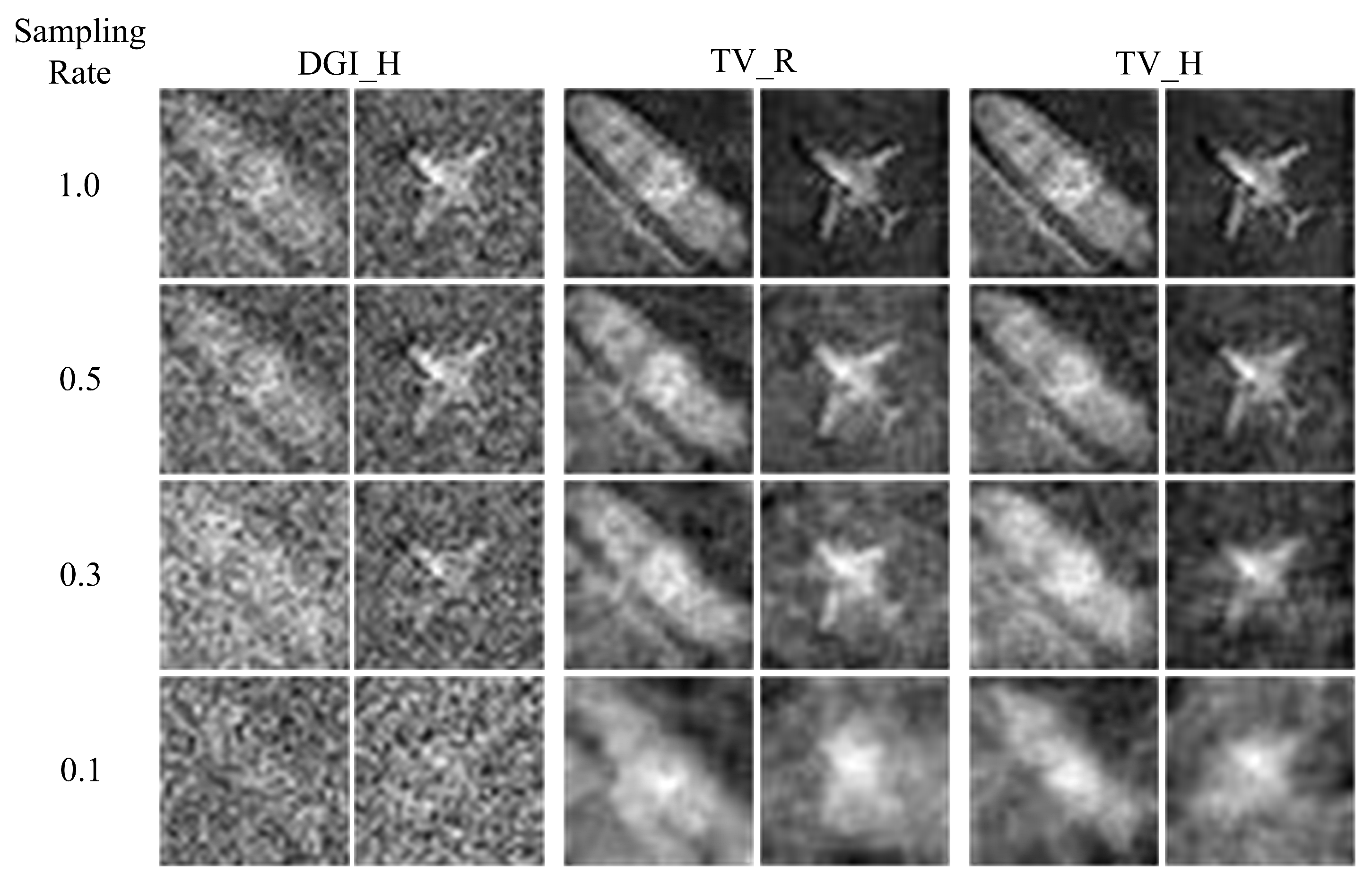
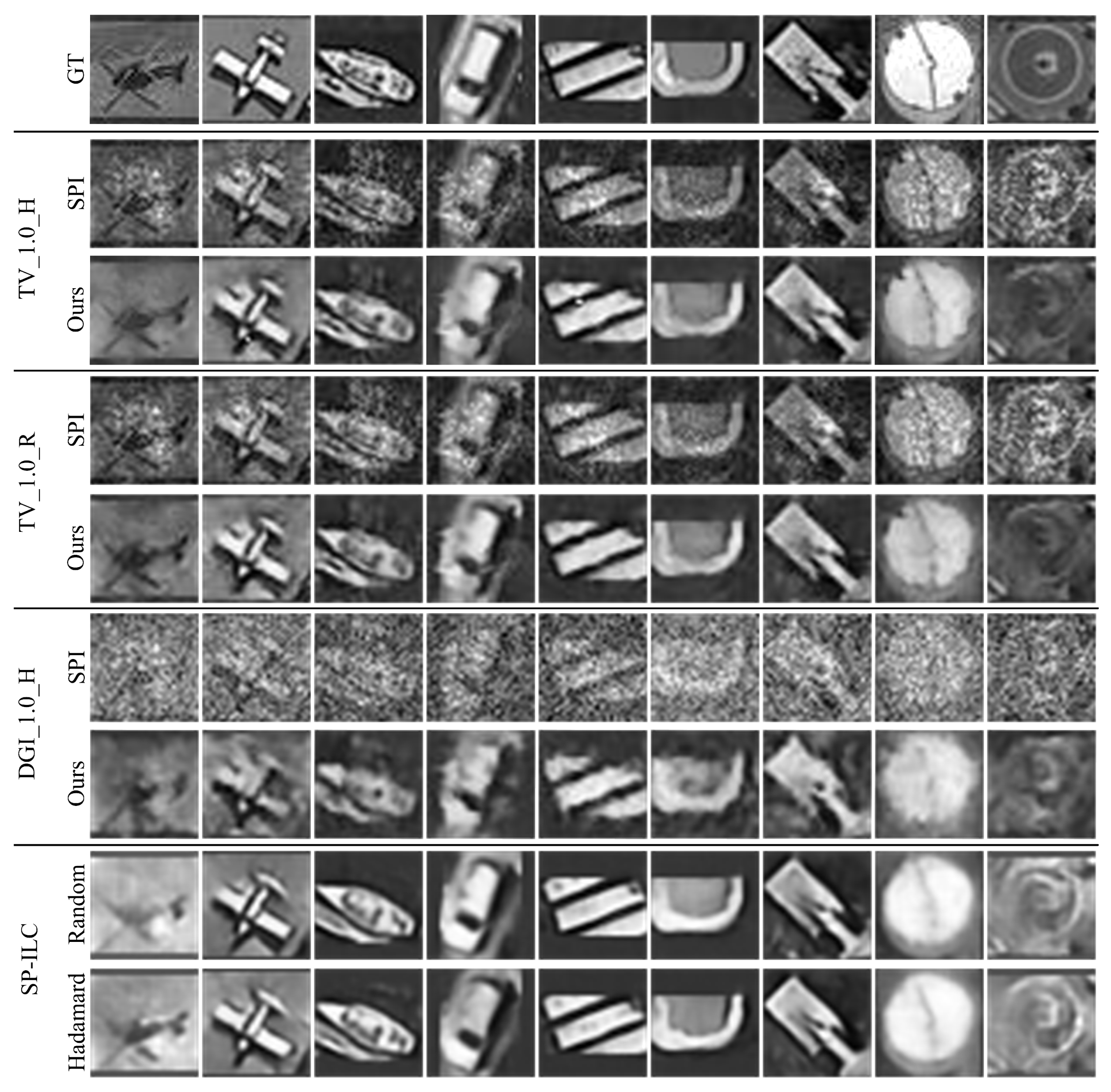
3.3. Image Quality Enhancement

Since our method adopts a dual-task learning principle, it not only improves the robustness and classification accuracy of the network but also enhances the quality of SPI reconstruction images, providing high-quality turbulence-free images for subsequent computer vision tasks. To assess image quality restoration, we conducted experiments on the validation sets across all datasets. Among the several methods, SP-ILC is image-free. Thus, the reconstructions are obtained directly using SP-ILC with SPI measurements.

The restoration effect of image quality is shown in Figure 8. The experimental results demonstrate that, compared to SPI, our network effectively mitigates turbulence effects, restoring object details and textures, while also enhancing image contrast and sharpness. This significantly improves the quality of SPI-reconstructed images on various objects. Across different datasets, the restoration performance of TV_1.0_H and TV_1.0_R is similar. However, TV_1.0_H exhibits superior restoration quality compared to DGI_1.0_H. This indicates that image-based restoration methods are highly influenced by the initial quality of SPI reconstruction. The distortion at the edges of vehicles and artifacts near the wings of aircrafts further support this conclusion. In contrast, SP-ILC based on image-free demonstrates superior performance in suppressing edge distortion and turbulence. This suggests that image-free reconstruction methods can establish a new mapping from measurements to images, eliminating the dependency on the initial quality of the reconstruction. Note that, although SP-ILC presents a nice reconstruction performance here, we have different observations in optical experiments. More detail will be provided in the Section 5.

We adopted two metrics, PSNR and SSIM, to evaluate the image quality enhancement performance. PSNR primarily performs pixel-level evaluation of the global distortion of an image. A higher PSNR value indicates a higher signal-to-noise ratio between the restored image and the ground truth, implying less distortion. SSIM primarily assesses the local structural similarity of an image, including luminance similarity, contrast similarity, and structural similarity. A higher SSIM value indicates a higher structural similarity between the restored image and the ground truth. In this experiment, image restoration was performed on all images in the validation set and the average PSNR and SSIM values were calculated. From the experimental results in

Table 2. The PSNR and SSIM of the restored images in the TV_1.0_H dataset.

Object	PSNR		SSIM
	Degraded	Restored	Degraded	Restored
Swimming pool	13.67	16.35	0.25	0.34
Ship	16.98	21.14	0.66	0.79
Helicopter	12.80	14.97	0.11	0.18
Storage tank	12.80	20.86	0.39	0.65
Small vehicle	17.02	21.92	0.61	0.76
Roundabout	14.50	19.66	0.10	0.24
Harbor	17.86	21.57	0.52	0.63
Plane	15.64	20.91	0.61	0.73
Large vehicle	15.78	20.43	0.69	0.82

, it can be observed that our network significantly improves image quality across all categories in the TV_1.0_H dataset, with an average increase in PSNR of 4.53 dB, reaching a maximum of 21.92 dB. The average SSIM improvement is 0.13, reaching a maximum of 0.82. For the DGI_1.0_H dataset, as shown in

Table 3. The PSNR and SSIM of the restored images in the DGI_1.0_H dataset.

Object	PSNR		SSIM
	Degraded	Restored	Degraded	Restored
Swimming pool	12.61	15.72	0.17	0.30
Ship	13.03	17.94	0.39	0.63
Helicopter	12.66	14.87	0.11	0.17
Storage tank	13.27	18.97	0.22	0.57
Small vehicle	12.60	18.94	0.35	0.61
Roundabout	14.38	19.24	0.10	0.23
Harbor	13.14	19.28	0.31	0.50
Plane	14.54	17.80	0.38	0.56
Large vehicle	12.43	17.37	0.40	0.69

, the PSNR increases by an average of 4.61 dB, with a maximum of 19.28 dB. Similarly, the SSIM increases by an average of 0.2, with a maximum of 0.69. These results indicate that, given the relatively weaker reconstruction performance of DGI compared to TV, the improvement margins on the DGI_1.0_H dataset are notably higher than those on the TV_1.0_H dataset, showing that our method provides substantial enhancement for low-quality images and demonstrates strong robustness. Furthermore, according to

Table 4. The PSNR and SSIM of all datasets.

Dataset	PSNR		SSIM
	Degraded	Restored	Degraded	Restored
TV_1.0_H	15.99	20.57	0.55	0.68
TV_0.5_H	15.44	18.84	0.50	0.60
TV_0.3_H	14.55	16.69	0.45	0.51
TV_0.1_H	12.43	14.78	0.32	0.35
TV_1.0_R	16.11	20.26	0.54	0.67
TV_0.5_R	15.43	18.76	0.50	0.59
TV_0.3_R	14.52	17.04	0.45	0.51
TV_0.1_R	12.39	14.77	0.32	0.35
DGI_1.0_H	13.03	18.01	0.32	0.56
DGI_0.5_H	13.01	16.40	0.35	0.56
DGI_0.3_H	11.74	14.46	0.24	0.43
DGI_0.1_H	10.68	13.85	0.14	0.32

, the average PSNR improvement across datasets is 3.26 dB, and the average SSIM improvement is 0.12, with peak improvements of 4.98 dB in PSNR and 0.24 in SSIM. For the same single-pixel reconstruction algorithm, the magnitude of improvement in image quality decreases as the sampling rate decreases, which is in agreement with theoretical expectations. For different reconstruction algorithms at the same sampling rate, images reconstructed using TV achieve better restoration results than those reconstructed using DGI. In summary, these experimental results fully demonstrate the effectiveness of our method in different single-pixel reconstruction schemes.

4. Ablation Study

To ensure the feasibility of LR-DTSPNet, we performed component-wise ablation analyses through systematic removal of critical modules, generating three controlled architectural variants for comparative evaluation. Among them, “w/o Swin–Conv Block” removes the Swin–Conv Block, “w/o C2f Block” removes the C2f Block, and “w/o dualtask learning” retains only the object classification task. The results of the ablation study are shown in Figure 9. The findings indicate that the elimination of certain components results in different levels of performance decline. The most significant performance drop occurs when dual-task learning is removed, with a maximal accuracy decrease of 5.24% and an average decrease of 4.77%. The second most significant impact is observed when the C2f Block is removed, resulting in a maximal accuracy decrease of 2.94% and an average decrease of 1.82%. Still in terms of classification accuracy, removal of the Swin–Conv Block has the least impact, with a maximum accuracy decrease of 0.21% and an average decrease of 0.085%.

We also compared the performance drops in terms of image restoration. The results are summarized in

Table 5. Comparison of PSNR and SSIM with other variants.

Dataset	PSNR/SSIM
	Full Model	w/o Swin–Conv Block	w/o C2f Block
TV_1.0_H	20.57/0.68	19.16/0.66	20.40/0.68
TV_0.5_H	18.84/0.60	15.22/0.56	17.29/0.57
TV_0.3_H	16.69/0.51	13.93/0.48	16.28/0.51
TV_0.1_H	14.78/0.35	14.07/0.35	13.00/0.33

. We did not perform the “w/o dual-task learning” test, because the classification task is primary and the image restoration task would be removed in this case. The findings reveal that the variant “w/o Swin–Conv Block” exhibited an average PSNR reduction of 2.13 dB and an average SSIM reduction of 0.02. Similarly, the “w/o C2f Block” variant resulted in an average PSNR reduction of 0.98 dB and an average SSIM reduction of 0.01. The ablation study demonstrates that all three components play crucial roles. The Swin–Conv Block contributes more significantly to image restoration, while dual-task learning has a greater impact on object classification. C2f Block significantly aids in object classification, being more impactful in addition to dual-task learning.

In addition, compared to the classification network in YOLOv8s, we removed one C2f Block. Experimental results indicate that, for low-resolution images degraded by turbulence, removing a C2f Block not only substantially reduces the model’s parameter count and free up resources in our backbone network, but also keeps the classification accuracy without significantly degrade. In Figure 10, it is illustrated that while our classification network experiences a minimal drop in accuracy of only 0.22% on the same dataset, it significantly decreases the parameter count by 3.34 million. Therefore, our classification network employs only three C2f Blocks. This configuration, combined with our backbone network, achieves a higher classification accuracy than YOLOv8s while maintaining a lower parameter count.

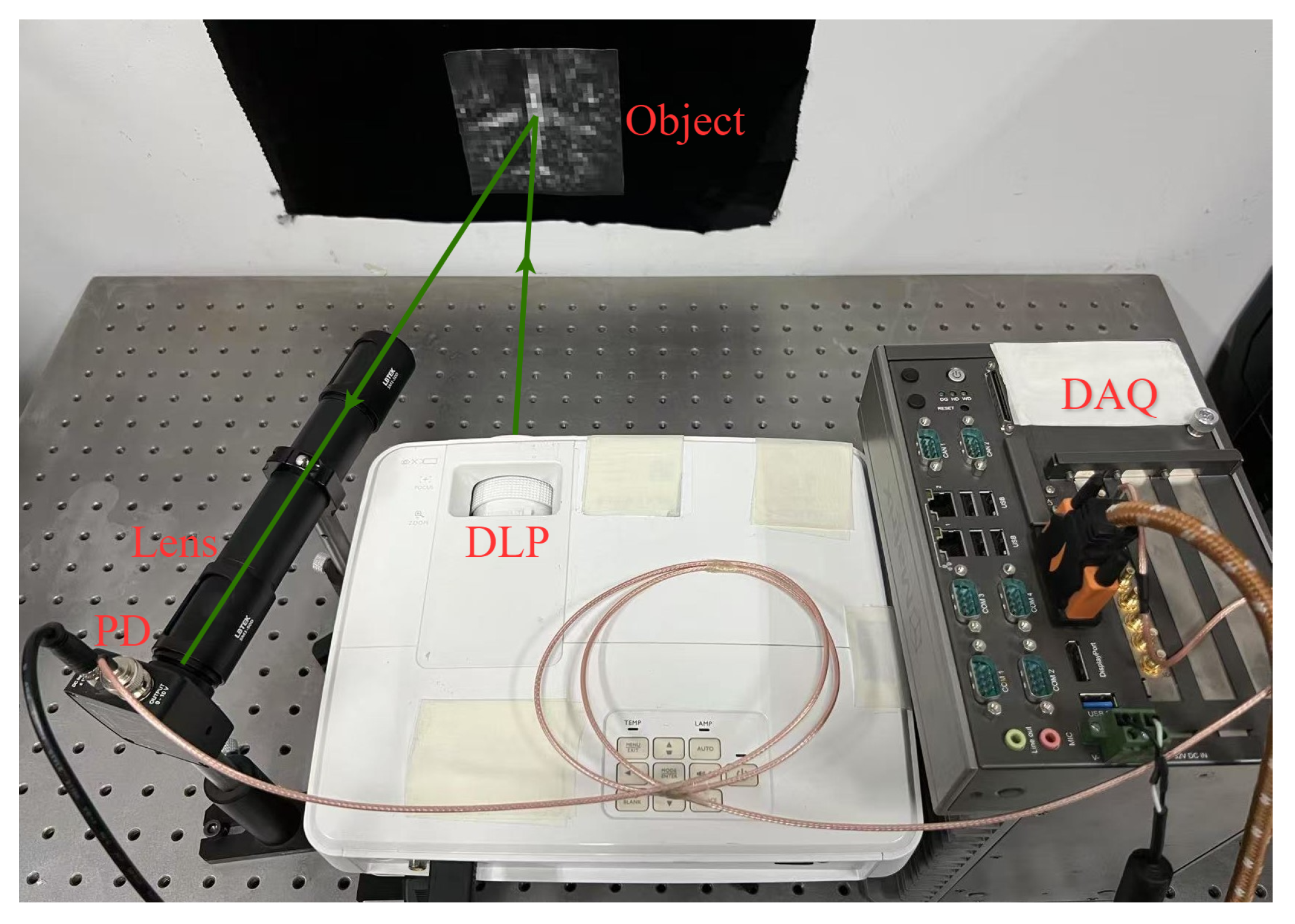
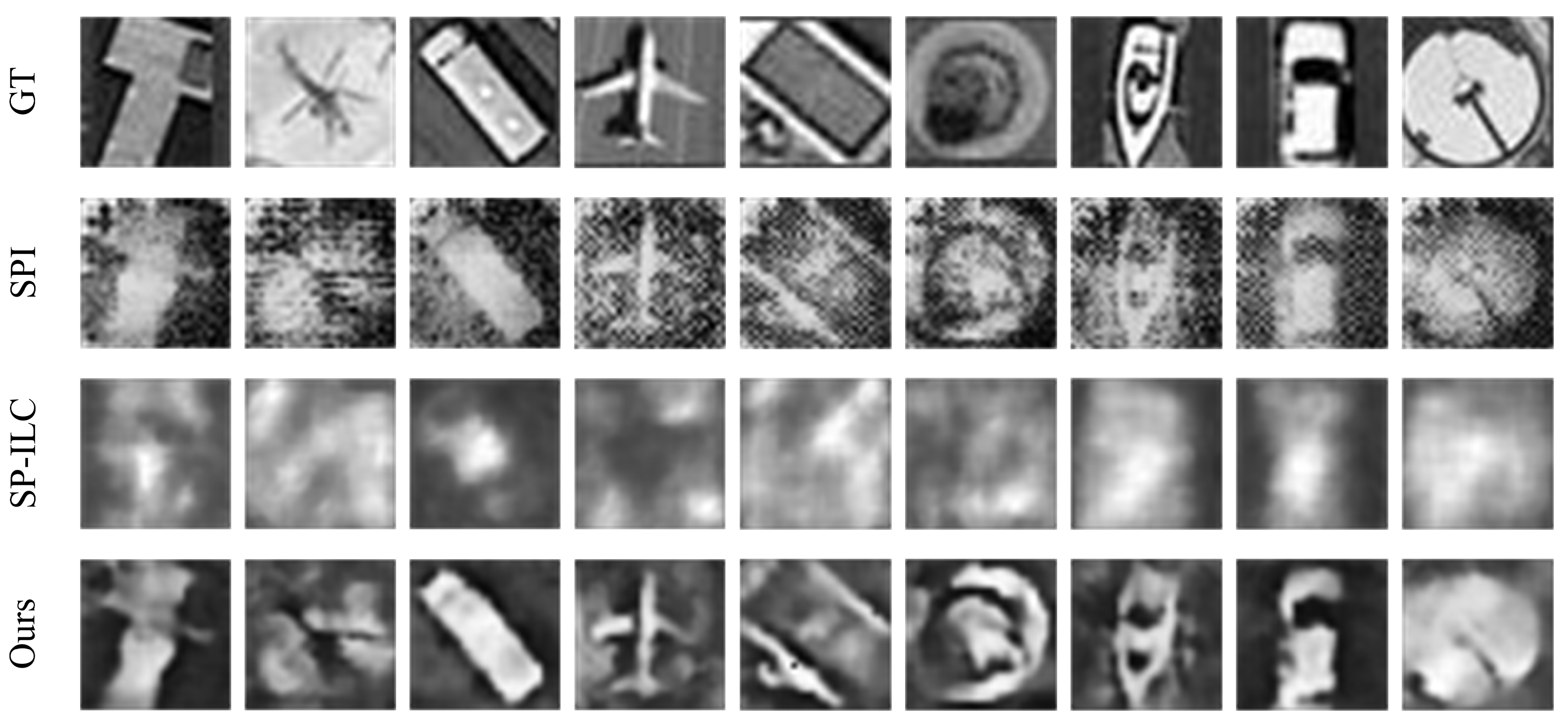
5. Optical Experiments

The setup of the optical experiment is shown in Figure 11. Modulation patterns are loaded onto a digital light projector (DLP) and projected onto the object. After interacting with the degraded image, the modulated light field is focused by a lens group onto a photo detector (PD, DH-GDT-D020V, Daheng optics, Beijing, China) to capture a one-dimensional bucket signal. This one-dimensional signal is then processed by a data acquisition card (DAQ, ADLINK PCIe-9814, ADLINK, Beijing, China) and stored on a computer. Since the cake-cutting Hadamard patterns exhibit excellent feature extraction capabilities, we employed these patterns as modulation patterns in the experiment. Furthermore, the sampling rates for the experiment are 100%, 50%, 30%, and 10%.

During the experiment, we observed that DGI demonstrated stronger noise resistance compared to TV. Consequently, we selected DGI for image reconstruction. After reconstructing the object images using DGI, we mixed the optical experimental images with simulated ones in a 1:1 ratio to expand the dataset and prevent the neural network from overfitting. The resulting dataset consists of 1760 images for training and 440 images for testing. During the network training process, MobileNetV3, ViT, YOLOv8s, SP-ILC, and our network each loaded pre-trained model parameters derived from the simulated dataset. The test datasets used in the experiments were excluded from the training. After 400 training epochs, the comparative results of the networks are shown in Figure 12.

The results show that our network achieves significantly higher classification accuracy compared to other classification networks with different sampling rates. For image-based object classification methods, our method achieves an average improvement of 8.21%. Moreover, as the sampling rate decreases from 100% to 30%, our network maintains high accuracy, demonstrating its exceptional robustness. Specifically, at a sampling rate of 30%, our network achieved a 9.6% higher accuracy compared to YOLOv8s, which is impressive. Compared to image-free SP-ILC, our method achieved more than double the classification accuracy, with an average improvement of 42.56%. For the performance decline in experimental results compared to simulated ones, we attribute it primarily to two factors. Firstly, the low resolution of our reconstructed images led to significant loss of details and textures, exacerbated by further magnification in optical experiments. Secondly, the experimental system introduced additional noise, leading to considerable reconstruction errors. However, our method still demonstrates superior performance compared to other classification networks.

Furthermore, our network improves the quality of single-pixel images while performing classification, as illustrated in Figure 13. Compared to SPI, our network significantly improves image quality, effectively suppressing noise, enhancing object prominence, and refining image details. Additionally, compared to the reconstruction performance of SP-ILC, our restoration results are noticeably superior. The primary reason is that our simulation experiments solely included atmospheric turbulence phase screens, without additional noise, resulting in relatively ideal conditions. However, in optical experiments, the restoration quality may degrade significantly, especially for image-free classification methods using one-dimensional measurements. In contrast, image-based methods, with their twostage process, exhibit greater noise resistance and robustness in practical scenarios. For objects such as harbors, vehicles, airplanes, and ships, the background becomes cleaner after network processing, and the distinctive features of each object are more prominently highlighted, which supports improved performance in subsequent computer vision tasks. These experimental results confirm the superior performance of our proposed method in both object classification and image quality restoration tasks.

6. Conclusions

This paper proposes a single-pixel long-range object classification method based on dual-task learning, specifically addressing atmospheric turbulence. The network backbone incorporates Swin–Conv Blocks into a UNet architecture, enhancing the network’s capability for both local and global feature extraction from turbulent degraded images. Additionally, by adopting the concept of dual-task learning, our method unifies image object classification and quality restoration tasks under a shared backbone, which not only improves classification accuracy and network robustness, but also provides high-quality restored images for downstream visual tasks. Both simulated and experimental results validate the excellent performance of our proposed method, demonstrating remarkable robustness and providing a promising solution for low-resolution image classification under turbulent conditions.

Despite the fact that our method shows a significant improvement in optical experiments, some limitations remain. Specifically, in tasks involving image quality restoration, the output images are still affected by distortions at the edges, such as harbor. Therefore, in future work, we will address these issues by refining both imaging systems and processing algorithms. Additionally, we aim to further optimize the method for classification accuracy, robustness, and real-time performance to adapt to more challenging turbulent environments.

References

1. Kechagias-Stamatis, O.; Aouf, N. Automatic target recognition on synthetic aperture radar imagery: A survey. IEEE Aerosp. Electron. Syst. Mag. 2021, 36, 56–81. [Google Scholar] [CrossRef]
2. Huizing, A.; Heiligers, M.; Dekker, B.; De Wit, J.; Cifola, L.; Harmanny, R. Deep learning for classification of mini-UAVs using micro-Doppler spectrograms in cognitive radar. IEEE Aerosp. Electron. Syst. Mag. 2019, 34, 46–56. [Google Scholar]
3. Jiang, H.; Diao, Z.; Shi, T.; Zhou, Y.; Wang, F.; Hu, W.; Zhu, X.; Luo, S.; Tong, G.; Yao, Y.D. A review of deep learning-based multiple-lesion recognition from medical images: Classification, detection and segmentation. Comput. Biol. Med. 2023, 157, 106726. [Google Scholar] [CrossRef]
4. Penumuru, D.P.; Muthuswamy, S.; Karumbu, P. Identification and classification of materials using machine vision and machine learning in the context of industry 4.0. J. Intell. Manuf. 2020, 31, 1229–1241. [Google Scholar] [CrossRef]
5. Li, X.; Yan, L.; Qi, P.; Zhang, L.; Goudail, F.; Liu, T.; Zhai, J.; Hu, H. Polarimetric imaging via deep learning: A review. Remote Sens. 2023, 15, 1540. [Google Scholar] [CrossRef]
6. Zhu, Z.; Li, X.; Zhai, J.; Hu, H. PODB: A learning-based polarimetric object detection benchmark for road scenes in adverse weather conditions. Inf. Fusion 2024, 108, 102385. [Google Scholar] [CrossRef]
7. Li, B.; Chen, Z.; Lu, L.; Qi, P.; Zhang, L.; Ma, Q.; Hu, H.; Zhai, J.; Li, X. Cascaded frameworks in underwater optical image restoration. Inf. Fusion 2025, 117, 102809. [Google Scholar] [CrossRef]
8. Wang, F.; Wang, C.; Deng, C.; Han, S.; Situ, G. Single-pixel imaging using physics enhanced deep learning. Photonics Res. 2021, 10, 104–110. [Google Scholar] [CrossRef]
9. Li, Z.; Huang, J.; Shi, D.; Chen, Y.; Yuan, K.; Hu, S.; Wang, Y. Single-pixel imaging with untrained convolutional autoencoder network. Opt. Laser Technol. 2023, 167, 109710. [Google Scholar] [CrossRef]
10. Huang, J.; Li, Z.; Shi, D.; Chen, Y.; Yuan, K.; Hu, S.; Wang, Y. Scanning single-pixel imaging lidar. Opt. Express 2022, 30, 37484–37492. [Google Scholar] [CrossRef]
11. Zhang, P.; Gong, W.; Shen, X.; Han, S. Correlated imaging through atmospheric turbulence. Phys. Rev. A—Atomic Mol. Opt. Phys. 2010, 82, 033817. [Google Scholar] [CrossRef]
12. Xu, Y.K.; Liu, W.T.; Zhang, E.F.; Li, Q.; Dai, H.Y.; Chen, P.X. Is ghost imaging intrinsically more powerful against scattering? Opt. Express 2015, 23, 32993–33000. [Google Scholar] [PubMed]
13. Li, M.; Mathai, A.; Lau, S.L.; Yam, J.W.; Xu, X.; Wang, X. Underwater object detection and reconstruction based on active single-pixel imaging and super-resolution convolutional neural network. Sensors 2021, 21, 313. [Google Scholar] [CrossRef] [PubMed]
14. He, Z.; Dai, S.; Huang, L. Research on single-pixel imaging method in the complex environment. Optik 2022, 271, 170153. [Google Scholar]
15. Cao, J.; Nie, W.; Zhou, M. A high-resolution and low-cost entangled photon quantum imaging framework for marine turbulence environment. IEEE Netw. 2022, 36, 78–86. [Google Scholar] [CrossRef]
16. Deng, Z.; Zhang, Z.; Xiong, S.; Wang, Q.; Zheng, G.; Chang, H.; Zhong, J. Seeing through fire with one pixel. Opt. Lasers Eng. 2024, 183, 108540. [Google Scholar]
17. Zhang, T.; Xiao, Y.; Chen, W. Single-pixel microscopic imaging through complex scattering media. Appl. Phys. Lett. 2025, 126, 031106. [Google Scholar]
18. Shapiro, J.H. Computational ghost imaging. Phys. Rev. A—Atomic Mol. Opt. Phys. 2008, 78, 061802. [Google Scholar] [CrossRef]
19. Fu, Q.; Bai, Y.; Tan, W.; Huang, X.; Nan, S.; Fu, X. Principle of subtraction ghost imaging in scattering medium. Chin. Phys. B 2023, 32, 064203. [Google Scholar]
20. Wang, X.; Jiang, P.; Gao, W.; Liu, Z.; Li, L.; Liu, J. Long-distance ghost imaging with incoherent four-petal Gaussian sources in atmospheric turbulence. Laser Phys. 2023, 33, 096003. [Google Scholar]
21. Leihong, Z.; Zhixiang, B.; Hualong, Y.; Zhaorui, W.; Kaimin, W.; Dawei, Z. Restoration of single pixel imaging in atmospheric turbulence by Fourier filter and CGAN. Appl. Phys. B 2021, 127, 1–16. [Google Scholar]
22. Zhang, H.; Duan, D. Turbulence-immune computational ghost imaging based on a multi-scale generative adversarial network. Opt. Express 2021, 29, 43929–43937. [Google Scholar] [CrossRef]
23. Zhang, L.; Zhai, Y.; Xu, R.; Wang, K.; Zhang, D. End-to-end computational ghost imaging method that suppresses atmospheric turbulence. Appl. Opt. 2023, 62, 697–705. [Google Scholar] [PubMed]
24. Cheng, Y.; Liao, Y.; Zhou, S.; Chen, J.; Ke, J. Enhanced Single Pixel Imaging in Atmospheric Turbulence. In Proceedings of the Computational Optical Sensing and Imaging, Toulouse, France, 15–19 July 2024; CF1B. 5. Optica Publishing Group: Washington, DC, USA, 2024. [Google Scholar]
25. Wang, F.; Wang, H.; Wang, H.; Li, G.; Situ, G. Learning from simulation: An end-to-end deep-learning approach for computational ghost imaging. Opt. Express 2019, 27, 25560–25572. [Google Scholar] [PubMed]
26. Song, K.; Bian, Y.; Wu, K.; Liu, H.; Han, S.; Li, J.; Tian, J.; Qin, C.; Hu, J.; Xiao, L. Single-pixel imaging based on deep learning. arXiv 2023, arXiv:2310.16869. [Google Scholar]
27. Li, J.; Le, M.; Wang, J.; Zhang, W.; Li, B.; Peng, J. Object identification in computational ghost imaging based on deep learning. Appl. Phys. B 2020, 126, 1–10. [Google Scholar]
28. Zhang, Z.; Li, X.; Zheng, S.; Yao, M.; Zheng, G.; Zhong, J. Image-free classification of fast-moving objects using “learned” structured illumination and single-pixel detection. Opt. Express 2020, 28, 13269–13278. [Google Scholar]
29. Yang, Z.; Bai, Y.M.; Sun, L.D.; Huang, K.X.; Liu, J.; Ruan, D.; Li, J.L. SP-ILC: Concurrent single-pixel imaging, object location, and classification by deep learning. Photonics 2021, 8, 400. [Google Scholar] [CrossRef]
30. Peng, L.; Xie, S.; Qin, T.; Cao, L.; Bian, L. Image-free single-pixel object detection. Opt. Lett. 2023, 48, 2527–2530. [Google Scholar] [CrossRef]
31. Schmidt, J.D. Numerical Simulation of Optical Wave Propagation with Examples in MATLAB; SPIE: Bellingham, WA, USA, 2010. [Google Scholar]
32. Andrews, L.C. An analytical model for the refractive index power spectrum and its application to optical scintillations in the atmosphere. J. Mod. Opt. 1992, 39, 1849–1853. [Google Scholar]
33. Ferri, F.; Magatti, D.; Lugiato, L.A.; Gatti, A. Differential ghost imaging. Phys. Rev. Lett. 2010, 104, 253603. [Google Scholar] [PubMed]
34. Li, C. An Efficient Algorithm for Total Variation Regularization with Applications to the Single Pixel Camera and Compressive Sensing. Master’s Thesis, Rice University, Houston, TX, USA, 2010. [Google Scholar]
35. Bian, L.; Suo, J.; Dai, Q.; Chen, F. Experimental comparison of single-pixel imaging algorithms. J. Opt. Soc. Am. A 2017, 35, 78–87. [Google Scholar]
36. Caruana, R. Multitask learning. Mach. Learn. 1997, 28, 41–75. [Google Scholar]
37. Zhang, K.; Li, Y.; Liang, J.; Cao, J.; Zhang, Y.; Tang, H.; Fan, D.P.; Timofte, R.; Gool, L.V. Practical blind image denoising via Swin-Conv-UNet and data synthesis. Mach. Intell. Res. 2023, 20, 822–836. [Google Scholar]
38. Liu, Z.; Lin, Y.; Cao, Y.; Hu, H.; Wei, Y.; Zhang, Z.; Lin, S.; Guo, B. Swin transformer: Hierarchical vision transformer using shifted windows. In Proceedings of the IEEE/CVF International Conference on Computer Vision, Montreal, QC, Canada, 10–17 October 2021; pp. 10012–10022. [Google Scholar]
39. Xia, G.S.; Bai, X.; Ding, J.; Zhu, Z.; Belongie, S.; Luo, J.; Datcu, M.; Pelillo, M.; Zhang, L. DOTA: A large-scale dataset for object detection in aerial images. In Proceedings of the IEEE Conference on Computer Vision and Pattern Recognition, Salt Lake City, UT, USA, 18–22 June 2018; pp. 3974–3983. [Google Scholar]
40. Redmon, J.; Divvala, S.; Girshick, R.; Farhadi, A. You only look once: Unified, real-time object detection. In Proceedings of the IEEE Conference on Computer Vision and Pattern Recognition, Las Vegas, NV, USA, 27–30 June 2016; pp. 779–788. [Google Scholar]
41. Howard, A.; Sandler, M.; Chu, G.; Chen, L.C.; Chen, B.; Tan, M.; Wang, W.; Zhu, Y.; Pang, R.; Vasudevan, V.; et al. Searching for mobilenetv3. In Proceedings of the IEEE/CVF International Conference on Computer Vision, Seoul, Republic of Korea, 27 October–2 November 2019; pp. 1314–1324. [Google Scholar]
42. Woo, S.; Debnath, S.; Hu, R.; Chen, X.; Liu, Z.; Kweon, I.S.; Xie, S. Convnext v2: Co-designing and scaling convnets with masked autoencoders. In Proceedings of the IEEE/CVF Conference on Computer Vision and Pattern Recognition, Vancouver, BC, Canada, 17–24 June 2023; pp. 16133–16142. [Google Scholar]
43. Tan, M.; Le, Q. Efficientnetv2: Smaller models and faster training. In Proceedings of the International Conference on Machine Learning, Virtual, 18–24 July 2021; PMLR: Cambridge, MA, USA, 2021; pp. 10096–10106. [Google Scholar]
44. Dosovitskiy, A.; Beyer, L.; Kolesnikov, A.; Weissenborn, D.; Zhai, X.; Unterthiner, T.; Dehghani, M.; Minderer, M.; Heigold, G.; Gelly, S.; et al. An image is worth 16 × 16 words: Transformers for image recognition at scale. arXiv 2020, arXiv:2010.11929. [Google Scholar]
45. Wang, C.Y.; Liao, H.Y.M.; Wu, Y.H.; Chen, P.Y.; Hsieh, J.W.; Yeh, I.H. CSPNet: A new backbone that can enhance learning capability of CNN. In Proceedings of the IEEE/CVF Conference on Computer Vision and Pattern Recognition Workshops, Seattle, WA, USA, 14–19 June 2020; pp. 390–391. [Google Scholar]
Figure 1. The principle of dual-task learning.
Electronics 14 01355 g001
Figure 2. LR-DTSPNet Architecture.
Electronics 14 01355 g002
Figure 3. The architectures of sub-modules. In order, (ac) illustrate the structural schematics of the Swin–Conv Block, C2f Block, and Classification Head.
Electronics 14 01355 g003
Figure 4. The reconstruction results of different reconstruction schemes. “H” represents Hadamard pattern; “R” represents random pattern.
Electronics 14 01355 g004
Figure 5. Architectures of YOLO and ViT. (a) Backbone module of YOLO. (b) Transformer encoder of ViT.
Electronics 14 01355 g005
Figure 6. Results of simulated experiment: (ac), respectively, show the classification results of our method and common object classification methods on the TV_H, DGI_H, and TV_R datasets, while (d) shows the classification results of the image-free object classification method.
Electronics 14 01355 g006
Figure 7. Attention maps of degraded images.
Electronics 14 01355 g007
Figure 8. Results of image quality restoration. GT represents the ground truth.
Electronics 14 01355 g008
Figure 9. Comparison with other variants on the TV_H dataset.
Electronics 14 01355 g009
Figure 10. Classification results of classification network between YOLOv8 and ours.
Electronics 14 01355 g010
Figure 11. Setup of experimental system.
Electronics 14 01355 g011
Figure 12. Classification accuracy on the experimental dataset.
Electronics 14 01355 g012
Figure 13. Results of experimental image quality restoration.
Electronics 14 01355 g013