DIMK-GCN: A Dynamic Interactive Multi-Channel Graph Convolutional Network Model for Intrusion Detection

Abstract

Existing network intrusion detection models effectively capture relationships between nodes and extract key features. However, they often struggle to accurately represent node characteristics, particularly in modeling the spatiotemporal dynamics and topological structures with sufficient granularity. To address these limitations, we propose the dynamic interaction multi-channel graph convolutional network (DIMK-GCN), which integrates three key components: a spatiotemporal feature weighting module, an interactive graph feature fusion module, and a temporal feature learning module. The spatiotemporal feature weighting module constructs a dynamic graph structure that incorporates both nodes and edges, leveraging self-attention mechanisms to enhance critical feature representations. The interactive graph feature fusion module employs graph attention networks (GATs) to refine node relationships while integrating a multi-channel graph convolutional network (GCN) to extract multi-perspective features, thereby enhancing model depth and robustness. The temporal feature learning module utilizes gated recurrent units (GRUs) to effectively capture long-term dependencies and address challenges posed by non-stationary time series data. Experimental results on the CIC-IDS2017, CIC-IDS2018, and Edge-IIoTSet datasets demonstrate that DIMK-GCN significantly outperforms existing models in key performance metrics, including detection accuracy, recall, and F1-score. Notably, on the Edge-IIoTSet dataset, DIMK-GCN achieves an accuracy of 97.31%, verifying its effectiveness and robustness in detecting various types of network attacks.

1. Introduction

In recent years, the rapid development of network technology and the increasing complexity of attack methods have driven research in intrusion detection. Traditional feature engineering-based methods face limitations in handling massive high-dimensional traffic data, while the emergence of deep learning has introduced a new paradigm in this field. Ren et al. [1] proposed CANET, which enhances feature recognition capabilities through an attention mechanism. Building on this, Qazi et al. [2] integrated convolutional and recurrent structures to design the CRNN model, aiming to better capture dynamic features. To address resource-constrained scenarios, Liu et al. [3] innovatively transformed traffic data into images, simplifying the feature modeling process. Although these approaches have contributed to technological advancements, they still suffer from limitations such as insufficient dynamic feature modeling, inadequate utilization of spatiotemporal information, and weak noise resistance. To further exploit the spatiotemporal characteristics of network data, researchers have introduced spatiotemporal feature fusion techniques. Xu et al. [4] proposed the CNN-BiLSTM-Attention model, which combines bidirectional LSTM and an attention mechanism to enhance the processing of long sequential data. Additionally, Zhou et al. [5] proposed a lightweight intrusion detection model combining GRU and CNN, leveraging attention mechanisms and efficient convolutional structures to capture temporal dependencies and spatial features, enhancing both performance and efficiency. However, despite these improvements in short-term dependency modeling, challenges remain in long-term trend analysis and network topology exploration, warranting further optimization.

Graph neural network-based intrusion detection methods have seen remarkable advancements. Mittal K et al. [6] optimized IoT intrusion detection systems using a GCN-based ensemble model, improving detection performance. Lin L et al. [7] proposed the E-GRACL model, which integrates global attention and contrastive learning to enhance the graph representation of IoT traffic data. Jahin M A et al. [8] introduced CAGN-GAT Fusion, combining GAT and contrastive learning to improve feature learning capability and model generalization.

In terms of graph construction optimization, Tran D H et al. [9] proposed FN-GNN, which integrates GCN and SAGEConv to effectively optimize network flow data graph construction. Similarly, Abdullayeva F et al. [10] built an intrusion detection model for cloud computing environments using GCN and GraphSAGE. Additionally, Nowroozi E et al. [11] employed interval bound propagation (IBP) to enhance the adversarial robustness of deep neural networks, while Shojafar M et al. [12] combined ABC, PSO, and DE algorithms to optimize IDS classification accuracy and computational efficiency.

For mobile ad hoc networks (MANETs), Reka R et al. [13] developed the MSA-GCNN model incorporating the Coati optimization algorithm to mitigate node mobility and energy consumption issues, thereby improving multi-attack detection capabilities. Meanwhile, Altaf et al. [14] proposed the NE-GConv model, which enhances IoT intrusion detection efficiency through lightweight heterogeneous feature fusion (node–edge collaborative modeling); however, its reliance on manually defined topology rules and shallow architecture limits its ability to represent complex attacks. Wang et al. [15] introduced the tGCN-KNN model, which addresses data scarcity and structural information loss in small-sample intrusion detection by integrating dynamic graph modeling and triplet-based graph convolution with metric learning. Nevertheless, the model still faces challenges such as sensitivity to sample selection, bias in high-frequency node filtering, and insufficient adaptivity in edge weight adjustment.

Existing models in network intrusion detection effectively capture relationships between nodes and extract key features. However, they still face limitations in representing node characteristics, particularly in depicting the spatiotemporal dynamic complexity (e.g., variations in traffic patterns over time) and topological structure features (e.g., connection patterns and interaction relationships between nodes) with sufficient granularity. To address these challenges, this paper proposes a dynamic interaction multi-channel graph convolutional network (DIMK-GCN), which integrates spatiotemporal feature dynamic modeling and graph structure optimization mechanisms. This approach aims to enhance the adaptability of models to spatiotemporal evolution and improve their capability to capture complex interaction relationships. The framework of DIMK-GCN is illustrated in Figure 1.

The main contributions of this paper are as follows:

(1)

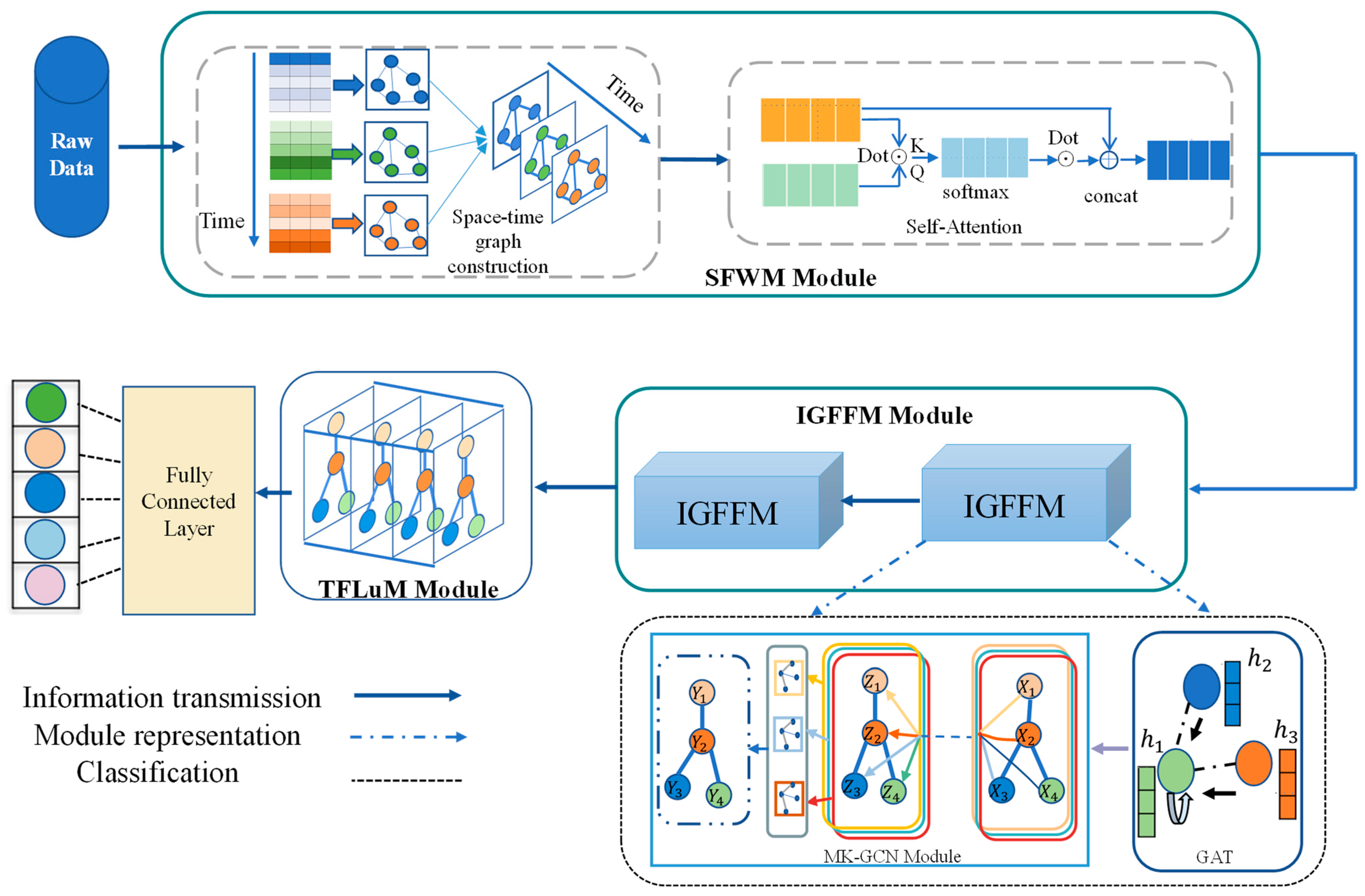
Proposal of the DIMK-GCN Model: We introduce the dynamic interaction multi-channel graph convolutional network (DIMK-GCN), which consists of a spatiotemporal feature weighting module, an interactive graph feature fusion module, and a temporal feature learning module, enhancing the model’s adaptability to spatiotemporal evolution data.

(2)

Construction of a Spatiotemporal Graph Structure: By integrating cosine similarity and a self-attention mechanism, we propose a precise feature weight allocation method to address the challenges of static connections and dynamic feature distribution, thereby improving the expressiveness of spatiotemporal features.

(3)

Optimization of Edge Weights in Graph Structures: We incorporate graph attention networks (GATs) and multi-kernel graph convolutional networks (MK-GCNs) to refine edge weights, enhance the capture of node interaction relationships, and improve the compactness and robustness of feature representation.

(4)

Introduction of GRUs for Temporal Feature Learning: By integrating gated recurrent units (GRUs), we overcome the limitations of traditional methods in capturing long-term dependencies and handling non-stationary time-series data, enhancing the model’s adaptability to evolving temporal patterns.

2. Materials

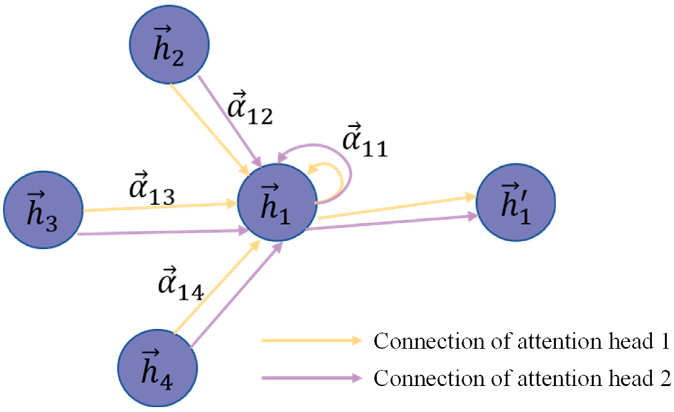
2.1. Graph Attention Networks

Graph attention networks (GATs) are an advanced neural network architecture designed for processing graph-structured data [16]. The structure of the GAT network is shown in Figure 2. GAT incorporates an attention mechanism that enables nodes to aggregate information from their neighbors based on dynamically learned importance weights.

Unlike traditional graph convolutional networks (GCNs), which rely on predefined adjacency matrices for message passing, GAT autonomously learns the importance of neighboring nodes through an attention coefficient, thereby enhancing its adaptability to complex graph structures. This property makes GAT particularly effective in tasks such as node classification, link prediction, and graph classification.

Given a vertex set $\mathrm{V}=\left\{v_i\right|i=1,2,\cdots ,N\}$, each vertex $v_i$ is associated with an initial feature vector $h_i\in {ℝ}^F$, where N represents the number of vertices and F denotes the dimensionality of the vertex features. A linear transformation is applied to the feature $h^{\prime }=Wh$ of each vertex, with W as a learnable weight matrix, resulting in the transformed feature representation $h_i^{\prime }\in {ℝ}^{F^{\prime }}$.

To enable the model to learn higher-level representations, GAT defines an attention mechanism $\alpha$, which is a single-layer feedforward neural network used to measure the correlation between vertices $v_i$ and $v_j$. Given the transformed feature vectors $h_i^{\prime }$ and $h_j^{\prime }$ of vertices $v_i$ and $v_j$, the attention coefficient $e_{ij}$ is computed as follows:

$$e_{ij}=\alpha (h_i^{\prime },h_j^{\prime })=LeakyReLU(a^T[h_i^{\prime }\oplus h_j^{\prime }])$$

(1)

In Equation (1), $e_{ij}$ represents the attention weight between node i and node j in the graph, measuring the strength of their connection. $h_i^{\prime },h_j^{\prime }$ denote the feature vectors of node i and j—their representations after transformation in the previous layer. LeakyReLU introduces nonlinear transformation, enabling the model to focus on smaller negative gradient information to enhance feature learning. $a^T$ is a trainable attention parameter vector for learning node relationships. $\oplus$ signifies vector concatenation, merging $h_i^{\prime }$ and $h_j^{\prime }$ into one vector.

To ensure the validity of the attention mechanism, the computed raw attention coefficients $e_{ij}$ must be normalized so that they become part of a probability distribution. This normalization is achieved through the Softmax function, which is defined as follows:

$${\alpha }_{ij}={\displaystyle \frac{\exp (e_{ij})}{{\displaystyle \sum _{k\in N_i\cup \left\{i\right\}}}\exp (e_{ik})}}$$

(2)

where ${\alpha }_{ij}$ is the normalized attention weight, indicating the degree of node $i’s$ attention to neighbor node j; $e_{ij}$ is the edge weight calculated by the attention mechanism; $N_i$ is the set of neighbor nodes of node I; and $N_i\cup \left\{i\right\}$ includes the neighborhood of node i itself. Based on the normalized attention weights ${\alpha }_{ij}$, the new vector representation of vertex $v_j$ can be obtained through a linear combination, written as follows:

$${\widehat{h}}_i=\sigma \left({\displaystyle \sum _{j\in N_i\cup \left\{i\right\}}{\alpha }_{ij}}{h}_j^{\prime }\right)$$

(3)

In Equation (3), ${\widehat{h}}_i$ represents the updated feature representation of node i. ${\alpha }_{ij}$ is the attention weight of node i toward neighbor node j. $h_j^{\prime }$ is the feature vector of neighbor node j. $\sigma (\cdot )$ is a nonlinear activation function, introducing nonlinear expressive ability. It aggregates neighbor information via weighted summation—here, the attention weight ${\alpha }_{ij}$ determines how much different neighbors affect the central node. Subsequently, the nonlinear transformation σ further enhances the model’s expressive capability.

2.2. Graph Convolutional Neural Networks

Graph convolutional networks (GCNs) are a type of deep learning model specifically designed to process graph-structured data [17], such as social networks, molecular structures, and more. GCNs define convolutional operations on graphs to aggregate node features with those of their neighbors, thereby learning node embeddings.

The core idea of GCNs is the aggregation of information from neighboring nodes. For each node in the graph, GCNs update its features by performing a weighted summation of the features of its neighboring nodes. This process can be regarded as a form of “convolution” operation on the graph, as illustrated in Figure 3, which shows the structure of the GCN.

Given a graph $G=(V,E)$, where V is the set of nodes and E is the set of edges, each node $v\in V$ is associated with a d-dimensional feature vector $x_v$, collectively forming the node feature matrix $X\in {ℝ}^{N\times d}$, where N represents the total number of nodes. The adjacency matrix A of the graph indicates the connections between nodes; if the edges are weighted, A becomes a weighted matrix. The degree matrix D is a diagonal matrix where each diagonal element $D_{ii}$ corresponds to the degree of node i, defined as the number of nodes directly connected to node i.

To prevent highly connected nodes from disproportionately influencing the results during feature aggregation, it is necessary to normalize the adjacency matrix. This normalization process leads to the updated node feature matrix H, as represented by Equations (4) and (5).

$$\tilde{A}=D^{-{\displaystyle \frac{1}{2}}}A{D}^{-{\displaystyle \frac{1}{2}}}$$

(4)

$$H=\sigma (\tilde{A}XW)$$

(5)

In Equation (4), $\tilde{A}$ is the normalized adjacency matrix, ensuring numerical stability in feature propagation. A is the original adjacency matrix, representing connection relationships among graph nodes. D is the degree matrix—its diagonal element $D_{ii}$ indicates the degree of node i. $D^{-{\displaystyle \frac{1}{2}}}$, the inverse square root of the degree matrix, balances the influence of nodes with varying degrees and prevents high-degree nodes from dominating feature updates.

In Equation (5),H denotes the updated node feature matrix; $\sigma$ is the activation function; $\tilde{A}$ represents the normalized adjacency matrix; X is the input node feature matrix; W serves as the weight matrix of this layer, performing linear transformation to map original features into a new feature space.

In graph convolution, the feature update for each node incorporates not only its own information but also the features of its neighboring nodes. This feature aggregation is achieved through the product of the normalized adjacency matrix $\tilde{A}$ and the node feature matrix X.

GCN can also stack multiple graph convolutional layers, where each layer performs a convolution operation on the output of the previous layer to learn more complex feature representations, written as follows:

$$H^{(l)}=\sigma (\tilde{A}{H}^{(l-1)}{W}^{(l-1)})$$

(6)

where $H^{(l)}$ is the output feature matrix of the l-th layer; $H^{(l-1)}$ is the node feature matrix of the $(l-1)-th$ layer, acting as the input; $W^{(l-1)}$ is the weight matrix of the $(l-1)-th$ layer.

2.3. Gated Recurrent Neural Network

Recurrent neural networks (RNNs) have garnered widespread attention for their exceptional performance in sequence learning tasks. However, they face challenges such as vanishing or exploding gradients when handling long-distance dependencies. To address these limitations, Cho et al. [18] proposed the gated recurrent units (GRUs), whose structure is illustrated in Figure 4 [19]. A GRU is a lightweight recurrent unit that retains the advantages of long short-term memory (LSTM) networks by simplifying its gating mechanisms while simultaneously reducing the number of parameters and computational costs.

The core operation of GRU revolves around dynamically regulating the flow of information through two crucial mechanisms: the “update gate” and the “reset gate”. The design of GRU aims to effectively handle long-term dependencies in sequential data while concurrently reducing the number of parameters.

At each time step t, the GRU receives the input vector $x_t$ and considers the hidden state $h_{t-1}$ from the previous time step The internal mechanism of GRU first calculates the update gate $z_t$, whose role is to determine the extent to which the old hidden state $h_{t-1}$ is retained in the new hidden state $h_t$ The calculation formula for the update gate is as follows:

$$z_t=\sigma (W_z{x}_t+U_z{h}_{t-1}+b_z)$$

(7)

In Equation (7), $z_t$ is the update gate vector, controlling the retention proportion of the previous hidden state $h_{t-1}$ at the current moment and determining the importance of past information; $x_t$ is the input feature vector at the current moment; $h_{t-1}$ is the previous hidden state, containing historical information; $W_z,U_z$ are trainable weight matrices, corresponding to the linear transformations of input $x_t$ and the previous hidden state $h_{t-1}$, respectively; $b_z$ is the bias term, adjusting the calculation result of the update gate; and $\sigma (\cdot )$ is the Sigmoid activation function, mapping the result to the interval $(0,1)$ to enable the update gate to smoothly control the information flow. The GRU computes the reset gate $r_t$, which determines the extent to which the old hidden state $h_{t-1}$ influences the candidate hidden state ${\tilde{h}}_t$ at the current time step. The reset gate is calculated in a manner similar to the update gate, written as follows:

$$r_t=\sigma (W_r{\mathrm{x}}_t+U_r{h}_{t-1}+b_r)$$

(8)

In Equation (8), $r_t$ is the reset gate vector, controlling the degree of forgetting the previous hidden state $h_{t-1}$ at the current moment and determining the influence of past information; $x_t$ is the current input feature vector; $h_{t-1}$ is the previous hidden state storing historical information; $W_r,U_r$ are trainable weight matrices acting on input $x_t$ and hidden state $h_{t-1}$ to control the reset gate calculation; and $b_r$ is the bias term adjusting the reset gate’s calculation result.

The GRU then proceeds to the calculation phase of the candidate hidden state. This state integrates the current input and the reset old state, and its formula is as follows:

$${\tilde{h}}_t=\tanh (W_h{x}_t+U_h(r_t\odot h_{t-1})+b_h)$$

(9)

In Equation (9), $W_h,U_h,b_h$ are weight matrices and bias terms and $\odot$ represents the Hadamard product (i.e., element-wise multiplication). The hyperbolic tangent function $\tanh$ serves as the activation function, ensuring the candidate hidden state values are within the range of $[-1,1]$.

Finally, the new hidden state $h_t$ is a weighted combination of the old hidden state and the candidate hidden state, with the weights given by the update gate $z_t$:

$$h_t=(1-z_t)\odot h_{t-1}+z_t\odot {\tilde{h}}_t.$$

(10)

In Equation (10), $h_t$ represents the hidden state at the current moment, indicating the model’s comprehensive memory of the current input and historical information. $z_t$ serves as the update gate, controlling the proportion of the historical state $h_{t-1}$ and the current candidate hidden state ${\tilde{h}}_t$ that the model retains. $h_{t-1}$ denotes the hidden state at the previous moment, which stores historical information. ${\tilde{h}}_t$ is the candidate hidden state, generated through the reset gate calculation using the current input $x_t$ and the previous hidden state $h_{t-1}$.

This process allows the GRU to selectively forget or retain old information as needed and update the hidden state based on the current input.

3. DIMK-GCN Network Model

To achieve fine-grained representation of spatiotemporal features in complex networks and improve the accuracy of network intrusion detection, we propose a dynamic interaction multi-channel graph convolutional neural network (DIMK-GCN). The DIMK-GCN consists of three main modules: ① a spatiotemporal feature weighting module (SFWM); ② an interactive graph feature fusion module (IGFFM); and ③ a temporal feature learning module (TFLuM).

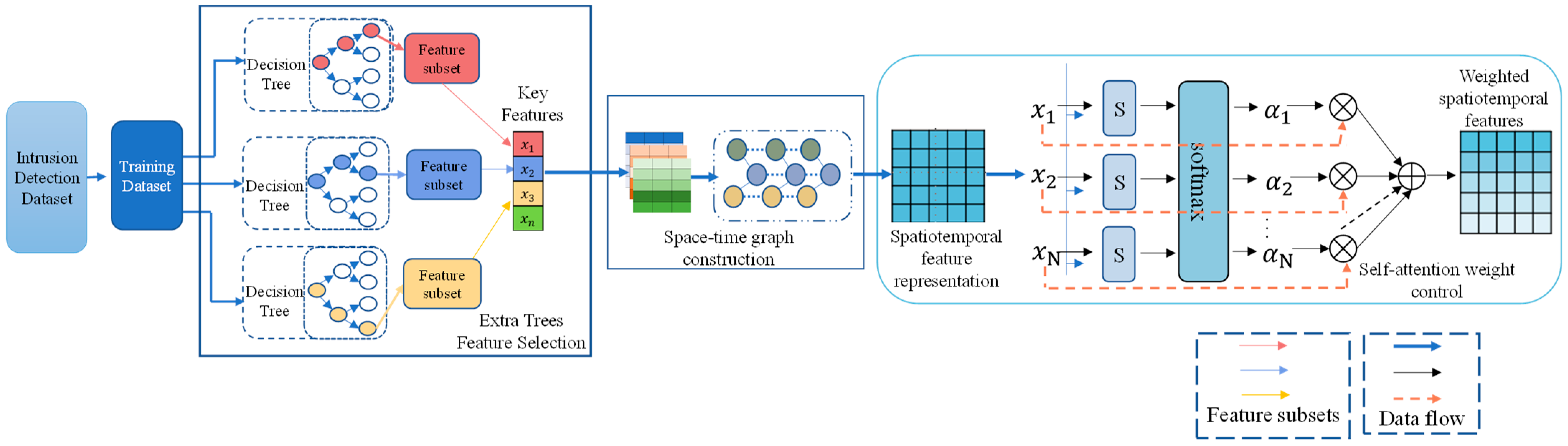
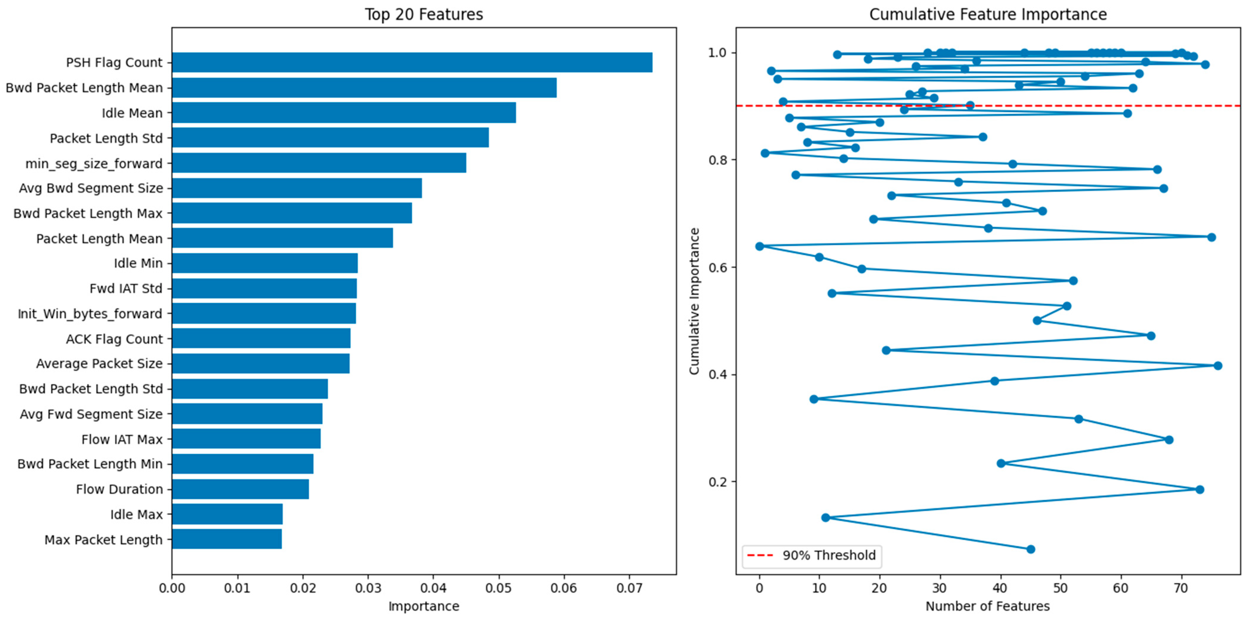
3.1. Spatiotemporal Feature Weighting Module

The spatiotemporal feature weighting module is designed to construct spatiotemporal graphs that effectively represent the characteristics of the data and to enhance the importance of key features using the self-attention mechanism. Its structure and process are shown in Figure 5, which illustrates the architecture of the spatiotemporal feature weighting module. First, the extra trees algorithm is employed for feature selection, extracting the most critical features for network intrusion detection to reduce interference from redundant information. Based on these features, a cosine similarity-based spatiotemporal graph is constructed. To further improve the feature representation capability, the self-attention mechanism is introduced, dynamically assigning weights to each feature by calculating the relationships between features. This strengthens the model’s focus on key features and provides a more accurate spatiotemporal representation for network intrusion detection.

The feature selection process using extra trees is a method based on an ensemble of random decision trees. Its core lies in evaluating the contribution of each feature to the model’s predictive ability.

First, a certain number of extra trees models are initialized and constructed. During the training phase of each tree, a subset of samples is randomly drawn from the complete dataset, and a random selection of features is used for node splitting. For each feature in each tree, its importance is measured by calculating the information gain obtained during the node-splitting process, i.e., the reduction in impurity. The formula for the reduction in Gini impurity is as follows:

$$\mathrm{Gain}(t,f)=\mathrm{Gini}(t_{\mathrm{before}})-{\displaystyle \sum _j\left(\frac{N_j}{N}\times \mathrm{Gini}(t_j)\right)}$$

(11)

where

• $t_{before}$ is the impurity of the node before splitting;
• $t_j$ represents the impurity of the j-th child node after the split;
• N is the total number of samples in the node before splitting;
• $N_j$ is the number of samples with impurity $t_j$ in the child node.

The feature gains from all trees are aggregated to obtain the overall importance of each feature are calculated as follows:

$$\mathrm{Importance}(f)={\displaystyle \frac{1}{T}}{\displaystyle \sum _{t=1}^T\mathrm{Gain}}(t,f)$$

(12)

where T represents the total number of trees and $\mathrm{Gain}(t,f)$ represents the gain of the feature.

All features are ranked based on the aggregated feature importance, and a subset is selected where the cumulative contribution reaches 90%. This threshold ensures the retention of key discriminative information while effectively reducing dimensional redundancy. As a result, 40 features were selected from the CIC-IDS2017 dataset and 32 features from the CIC-IDS2018 dataset. The selected features are partially shown in Figure 6 and Figure 7.

The spatiotemporal graph is a dynamic data structure used to capture and represent the feature changes of data at consecutive time points. In this study, the data at each intrusion detection time point is abstracted as a node in the graph. Cosine similarity is used to connect the nodes of the current time point with those of the preceding and succeeding time points to form cross-temporal edges, thus reflecting the dynamic associations in the time series.

The basic idea of spatiotemporal graph construction is as follows: First, an empty adjacency matrix is initialized based on the number of time points T and the number of nodes N at each time point. Then, the cosine similarity between each node and all nodes within a predefined window size is calculated. If the cosine similarity between two nodes exceeds a threshold, an edge is established between them, and the similarity is used as the edge weight. Finally, a graph structure is formed. The algorithm for constructing the spatiotemporal graph is described in Algorithm 1.

Algorithm 1: Spatiotemporal Graph Construction Algorithm

Input: X: Node feature matrix for all time steps, ${\{\mathrm{X}}_1,{\mathrm{X}}_2,\dots {\mathrm{X}}_T{\},\mathrm{X}}_{\mathrm{T}}\in R^{(N\times D)}$ T: Time step length $\theta$: Similarity threshold Output: A: Adjacency matrix for each time step, ${\{\mathrm{A}}_1,{\mathrm{A}}_2,\dots ,{\mathrm{A}}_T\}$ Steps:   1. G, X ← [], []   2. for t ← 1 to T do   3.   G[t] ← initialize_graph()   4.   V[t], E[t] ← initialize_nodes_and_edges()   5.   X[t] ← initialize_node_features()   6. end for   7. for t ← 1 to T do   8.   for i ∈ V[t] do   9.     for j ∈ V[t] where j ≠ i do   10.       if cosine_similarity(X[t][i], X[t][j]) > θ then E[t].add_edge(i, j)   11.     end for   12.     for Δt ∈ {−1, 1} do   13.       k ← t + Δt   14.       if 1 ≤ k ≤ T then   15.         for m ∈ V[k] do   16.           if cosine_similarity(X[t][i], X[k][m]) > θ then E[t].add_edge(i, m)   17.         end for   18.       end if   19.     end for   20.   end for   21.   G[t].set_edges(E[t])   22. end for   23. A ← [build_adjacency_matrix(G[t]) for t ← 1 to T]   24. return A

In the task of network intrusion detection, certain features may be highly correlated with attack behaviors, while others may be irrelevant or weakly correlated. The core advantage of the self-attention mechanism is its ability to adaptively adjust the weights of these features, enabling the model to focus on those most critical for attack detection.

First, the similarity between features is calculated using the query matrix Q the key matrix K as shown in the following Equation (13):

$$\mathrm{Attention} \mathrm{Score}=Q{K}^T$$

(13)

In Equation (13), $Q$ is the query matrix, representing the query part of input information—typically extracted from the feature representation at the current moment. $K$ is the key matrix, denoting the key—value part of input information, which matches the query part to calculate attention scores. $Q{K}^T$, the dot product of the query and the key, computes attention scores to measure the similarity between the query and the key.

Next, the similarity values are normalized using the softmax function, ensuring that the sum of weights for each feature is 1. The weight calculation is as follows:

$${\alpha }_{ij}=\mathrm{softmax}({\displaystyle \frac{Q_i{K}_j^T}{\sqrt{d_k}}})$$

(14)

In Equation (14), ${\alpha }_{ij}$ represents the weight between query feature $i$ and key feature $j$. $Q_i$ is the query vector (Query), indicating the feature representation of the current input element. $K_j$ is the key vector (Key), denoting reference information for matching with the query vector. $d_k$ is the dimension of the key vector, used to scale the dot—product value and avoid excessively large values. Softmax is employed to obtain the normalized attention distribution.

Finally, the calculated weights are applied to the value matrix V to obtain the weighted values. This weighted sum process allows the final representation of each feature to reflect its relationship with other features, as shown in the following Equation (15):

$$Outpu{t}_i={\displaystyle \sum _j{\alpha }_{ij}{V}_j}$$

(15)

In Equation (15), $Outpu{t}_i$ represents the final output at the query position $i$, resulting from the weighted average of all keys $K_j$ and their corresponding values $V_j$. ${\alpha }_{ij}$ is the attention weight defined in Equation (14). $V_j$ denotes the output information associated with the key vector $K_j$, reflecting the weighted result of the query position $i$ based on all keys $K_j$.

Through the self-attention mechanism, the model can effectively assign weights to each feature, reflecting their importance in the overall task. In the spatiotemporal graph construction module, this mechanism helps the model understand and highlight the attack topology in network intrusion detection data. By dynamically adjusting weights, the model can flexibly adapt to temporal changes in network traffic data, providing a solid foundation for subsequent feature fusion and temporal analysis.

The spatiotemporal feature weighting module refines network traffic representation by constructing a spatiotemporal graph and dynamically optimizing feature weights. First, the extra trees algorithm is used to select core features, reducing redundant interference. Next, cosine similarity is employed to construct the spatiotemporal graph, providing a structured representation. Finally, the self-attention mechanism dynamically assigns weights to enhance key feature representation. In summary, the spatiotemporal graph preserves spatiotemporal correlations in the data, while the self-attention mechanism optimizes feature weights dynamically, collaboratively improving feature discrimination in intrusion detection.

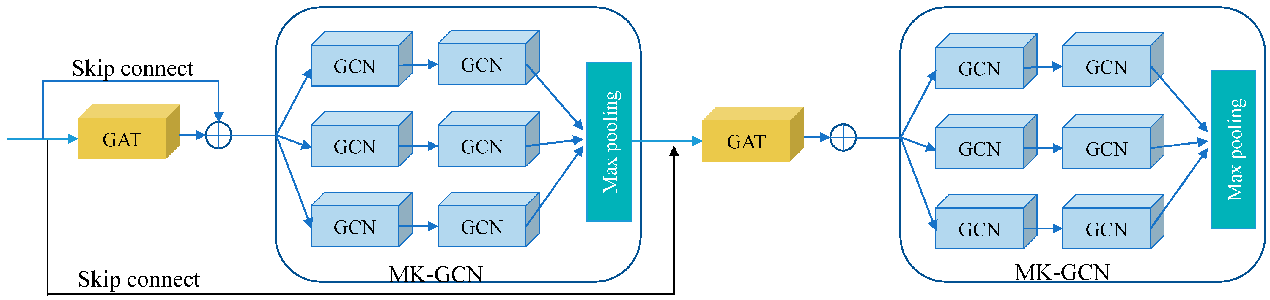
3.2. Interactive Graph Feature Fusion Module

The interactive graph feature fusion module (IGFFM) is primarily composed of GAT and MK-GCN, with two residual connections introduced to enhance feature transmission and stability. Its structure is depicted in Figure 8.

IGFFM further optimizes the node interaction relationships in the graph structure and extracts highly expressive feature representations based on the spatiotemporal feature weighting module. Specifically, the spatiotemporal feature weighting module constructs a spatiotemporal graph using cosine similarity and dynamically assigns feature weights through the self-attention mechanism, thereby providing the model with enhanced representations of key features. Based on this input, the IGFFM module further refines node feature representations and graph structure weights through the synergistic interaction of GAT and MK-GCN.

First, GAT extracts initial node features from the input graph and calculates dynamic weights between nodes using the attention mechanism, focusing on key neighboring node information. At the same time, a residual connection is introduced to directly add the original input features to the output of GAT, preserving initial information and mitigating potential information loss. Subsequently, the node features extracted by GAT are passed to MK-GCN, which enhances the learning ability for graph-structured data by introducing a set of parallel weight matrices to update the node feature matrix. Specifically, in MK-GCN, each node feature matrix is updated through three independent and parallel weight matrices, which extract node features from different perspectives, forming updated node feature matrices and expanding feature representation capabilities. Furthermore, MK-GCN incorporates the input features into its output through residual connections, enhancing feature consistency and model robustness. Finally, the node representations generated by MK-GCN are fed back to GAT, which recalculates attention weights based on the updated features to more precisely model the relationships between nodes. Through multiple iterations, GAT and MK-GCN mutually enhance each other, collaboratively optimizing node feature representations and global graph structure weights, providing highly expressive feature inputs for the subsequent temporal feature learning module.

To stabilize feature learning across layers, the model integrates Batch Normalization (BN), which standardizes layer inputs to zero mean/unit variance to mitigate internal covariate shift. Residual connections preserve critical information in deep architectures through skip connections that bypass intermediate layers. These are complemented by weight initialization (Xavier/He) and Adam optimization, forming a synergetic framework: BN stabilizes gradients, residuals prevent vanishing signals, and adaptive optimization ensures consistent convergence across layers.

Through multiple iterations, the model achieves deep learning of node relationships and high-order features. The model takes dynamic interactions between nodes as its core and uses the self-attention mechanism to accurately identify key node relationships, adaptively adjusting edge weights. This enables the model to fully capture the asymmetry of node associations in multi-feature spaces. Furthermore, by implementing multi-channel convolution for comprehensive feature extraction, the model continuously feeds rich feature information back into its internal structure, promoting the refinement of edge weights and feature representations in tandem.

3.2.1. Interactive Graph Feature Fusion

Given the graph-structured data, the initial node feature matrix, and the number of iterations, the iterative fusion process is as follows:

Step 1.

Initial feature extraction. First, GAT extracts initial node features from the input graph and calculates weights between nodes using the attention mechanism, emphasizing key neighboring node information.

Step 2.

Feature transmission. The node features calculated by GAT are passed to MK-GCN, which uses this information to extract rich representations of nodes from multiple feature spaces.

Step 3.

Feature feedback. The node representations extracted by MK-GCN are fed back to GAT, which recalculates attention weights based on the new node representations to refine node relationships.

Step 4.

Iterative optimization. The above process is iterated multiple times, with GAT and MK-GCN mutually enhancing each other, progressively optimizing node feature representations and node weights.

The specific implementation is described in Algorithm 2.

Algorithm 2: Interactive Graph Feature Fusion Module

Input: X: Initial node feature matrix; A: Adjacency matrix; ${\mathrm{W}}_{\mathrm{GAT}}$: Weight parameters for GAT; $W_{MK\_GCN}$: Weight matrix collection for MK-GCN; activation_GAT: Activation function type for GAT; activation_MKGCN: Activation function type for MK-GCN; num_iterations: Number of interaction iterations. Output: X_refined: Final refined node feature matrix Steps:   1. X_current ← X   2. A_hat ← Normalize Adjacency(A)   3. for iter ← 1 to num_iterations do   4.   X_GAT ← GATLayer(X_current, A, W_GAT, activation_GAT)   5.   H_MKGCN ← []   6.   for i ← 1 to 3 do   7.     H_i ← Activation(A_hat × (X_GAT × W_MKGCN[i]), activation_MKGCN)   8.     H_MKGCN.append(H_i)   9.   end for   10.   X_MKGCN ← MaxPool(H_MKGCN)   11.   X_current ← X_MKGCN   12. end for   13. return X_current

3.2.2. Edge Weight Learning with Graph Attention

In network intrusion detection, the importance of interactions between different nodes varies. To address this, the model introduces the attention mechanism to adaptively learn the relationships between nodes, thereby enhancing its understanding of the graph structure.

GAT is used to update edge weights in the graph structure. Specifically, GAT calculates attention coefficients between a node and its neighbors to weight the neighbor information when computing embeddings. The attention coefficient is calculated as follows (Equation (16)):

$${\alpha }_{v,u}={\displaystyle \frac{\exp \left(\mathrm{LeakyReLU}\left(a^T[W{h}_v\oplus W{h}_u]\right)\right)}{{\displaystyle \sum _{u^{\prime }\in N_v}\exp }(\mathrm{LeakyReLU}(a^T[W{h}_v\oplus W{h}_{u^{\prime }}]))}}$$

(16)

where W is the weight matrix, $\alpha$ is a learnable parameter vector in the attention mechanism, $\oplus$ denotes vector concatenation, and $N_v$ is the set of neighbors of node i.

The model employs LeakyReLU as the activation function to mitigate “dead neurons” caused by ReLU’s zero output for negative inputs. By introducing a small non-zero slope (α = 0.01) in the negative region, LeakyReLU preserves gradient flow for negative values, critical for GAT’s signed attention weight learning and preventing information loss in attention computations. Complementing this, He (Kaiming) initialization is adopted for weight parameters (Equation (17)).

$$W~\mathcal{N}\left(0,{\displaystyle \frac{2}{d_{in}}}\right)$$

(17)

In Equation (17), $d_{in}$ represents the dimension of input features and $\mathcal{N}$ denotes a Gaussian distribution with a mean of zero and a variance of ${\displaystyle \frac{2}{d_{in}}}$. This initialization method ensures the network maintains appropriate weight scales during the initial training phase, reduces gradient anomalies, and guarantees the stability and efficiency of the GAT structure.

3.2.3. Node Feature Learning with Multi-Channel Graph Convolution

MK-GCN enhances the learning ability for graph-structured data by introducing a set of parallel weight matrices to update the node feature matrix. Specifically, in MK-GCN, each node feature matrix is updated through three independent and parallel weight matrices. These weight matrices extract node features from different perspectives, forming updated node feature matrices.

For a graph $G=(V,E)$, where V is the set of nodes and E is the set of edges, each node $v\in V$ has a feature vector $h_v^{(l)}$, where l denotes the current layer. $\tilde{A}=A+I$ is defined as the normalized adjacency matrix, where A is the original adjacency matrix, and I is the identity matrix. The degree matrix D is a diagonal matrix with diagonal elements representing the degrees of nodes.

For each node v, three parallel weight matrices are used to update its feature vector, as shown in the following Equation (18):

$$h_{v,k}^{(l+1)}=\sigma \left({\displaystyle \sum _{u\in N(v)\cup \left\{v\right\}}{\tilde{D}}_{uu}^{-\frac{1}{2}}}{\tilde{A}}_{uv}{\tilde{D}}_{vv}^{-{\displaystyle \frac{1}{2}}}{h}_u^{(l)}{W}_k^{(l)}\right)$$

(18)

In Equation (18), $h_{v,k}^{(l+1)}$ represents the feature vector of node v in the (l + 1)-th layer, where k denotes different channels—each corresponding to a distinct weight matrix. N(v) is the neighbor set of node v; ${\tilde{D}}_{uu}^{-{\displaystyle \frac{1}{2}}}$ and ${\tilde{D}}_{vv}^{-{\displaystyle \frac{1}{2}}}$ are standardized graph adjacency matrices, used to avoid the influence discrepancy between nodes of different degrees; ${\tilde{A}}_{uv}$ is the adjacency matrix element between node u and node v; $h_u^{(l)}$ is the feature vector of node u in the l-th layer; and $W_k^{(l)}$ denotes the weight matrix for different channels in the l-th layer, controlling the feature transformation of each channel.

To ensure stable gradient propagation across layers and maintain consistent variance between input and output, the weights in the GCN part are initialized using Xavier (Glorot) initialization. The initial values of the weights are given in Equation (19).

$$W_k^{(l)}~\mathcal{U}\left(-{\displaystyle \frac{\sqrt{6}}{\sqrt{d_{in}+d_{out}}}},{\displaystyle \frac{\sqrt{6}}{\sqrt{d_{in}+d_{out}}}}\right)$$

(19)

In the Equation (19), $W_k^{(l)}$ represents the weight matrix for the k-th channel in the l-th layer. $u()$ denotes the uniform distribution. $d_{in}$ indicates the input dimension of the neural network in the l-th layer, while $d_{out}$ represents the output dimension of the neural network in the L-th layer.

The three updated feature vectors are concatenated to form a larger feature vector $h_v^{(l+1)}$, as shown in the following Equation (20):

$$h_v^{(l+1)}=\mathrm{concat}(h_{v,1}^{(l+1)},h_{v,2}^{(l+1)},h_{v,3}^{(l+1)})$$

(20)

Equation (20) states that $h_v^{(l+1)}$ represents the final feature representation of node vv at layer l + 1, which is formed by concatenating multiple channel feature vectors. Specifically $h_{v,1}^{(l+1)}$, $h_{v,2}^{(l+1)}$, and $h_{v,3}^{(l+1)}$ denote the feature representations of node vv in different channels at layer l + 1. The operation concat represents feature concatenation, combining multiple channel feature vectors into a unified feature representation.

Finally, the concatenated feature vector is mapped to a lower-dimensional space through a pooling layer to reduce redundancy and retain key features, as shown in the following Equation (21):

$$h_v^{(l+1)}=\mathrm{Pooling}\left(h_v^{(l)}\right)$$

(21)

In Equation (21), Pooling denotes the pooling operation, which reduces the dimensionality of the high-dimensional feature vector $h_v^{(l+1)}$ after concatenation, thereby extracting compact and information-rich feature representations.

The IGFFM optimizes graph feature representation through a bidirectional collaborative mechanism of GAT and MK-GCN. GAT extracts node features while preserving original information via the attention mechanism, whereas MK-GCN enhances feature diversity through multi-channel parallel learning. Node interaction modeling and multi-channel feature fusion strengthen the feature discrimination capability of graph-structured data, providing more robust feature inputs for subsequent temporal analysis.

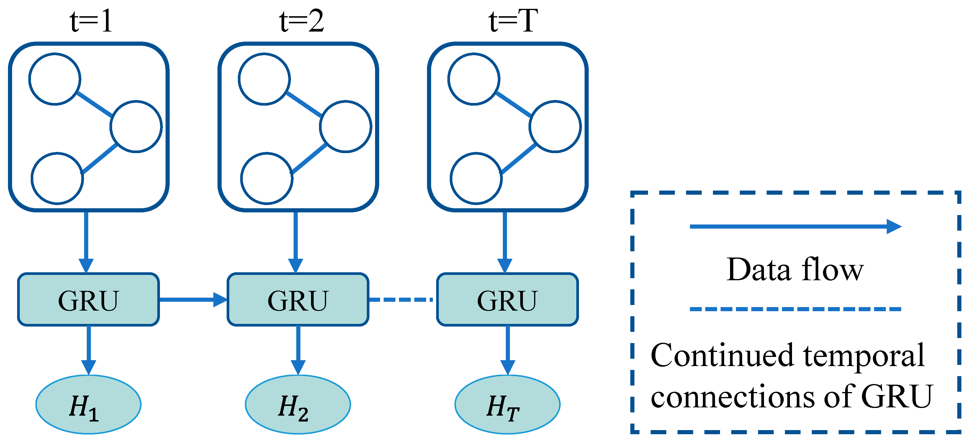
3.3. Temporal Feature Learning Module

The temporal feature learning module captures the complex relationships between data points in both spatial and temporal dimensions by constructing spatiotemporal graphs that link data points of adjacent time steps. This graph structure precisely expresses the dynamic relationships between time steps and provides spatiotemporal context for subsequent feature learning. Based on this, the model introduces the temporal feature learning module to capture the complex spatiotemporal dependencies and fuse spatiotemporal features through multi-layer graph convolution operations. The module is illustrated in Figure 9.

To comprehensively capture long-term and short-term temporal dependencies, the output sequence from the interactive graph feature fusion module is used as input. The temporal feature learning module learns and fuses global temporal information through its unique gating mechanism.

Let $G_t$ be the output vector generated by the interactive graph feature fusion module at time step t, representing the feature representation of complex relationships between data points in the local spatiotemporal graph structure.

$$G_{1:T}=\{G_1,G_2,\dots ,G_T\}$$

(22)

At each time step t, two gate values are first calculated: the reset gate $r_t$ and the update gate $z_t$. The reset gate determines the extent to which the previous hidden state $h_{t-1}$ should be forgotten in the current time step’s information update, while the update gate determines the fusion ratio between the new input and the previous memory. The formulas for these gates are as follows (Equations (23) and (24)):

$$r_t=\sigma (W_r\cdot [h_{t-1},G_t]+b_r)$$

(23)

$$z_t=\sigma (W_z\cdot [h_{t-1},G_t]+b_z)$$

(24)

where $W_r$ and $W_z$ are weight matrices, $b_r$ and $b_z$ are bias terms, and $\delta (\cdot )$ is the activation function.

Based on the reset gate, the candidate hidden state ${\tilde{h}}_t$ is calculated, representing the hidden state that would be produced if the past information were ignored. The formula for the candidate hidden state is as follows (Equation (25)):

$${\tilde{h}}_t=\tanh (W_h\cdot [r_t\odot h_{t-1},G_t]+b_h)$$

(25)

where $W_h$ is the weight matrix, $b_h$ is the bias term, and $\odot$ denotes element-wise multiplication.

Finally, the final hidden state ${\tilde{h}}_t$ is formed by integrating the past state $h_{t-1}$ and the new candidate hidden state based on the update gate $h_t$ (Equation (26)), written as follows:

$$h_t=(1-z_t)\odot h_{t-1}+z_t\odot {\tilde{h}}_t$$

(26)

The local spatiotemporal graph and interactive graph structure jointly enhance the ability to capture spatiotemporal information, while GRU deeply learns and fuses global temporal information through its gating mechanism. This fusion not only strengthens the model’s understanding of static relationships between nodes but also improves its sensitivity to dynamic changes in time series data.

In network traffic data, non-stationarity typically manifests as changes in data distribution over time. To address this issue, the temporal feature learning module adopts a design that combines spatiotemporal graphs and GRU to handle dynamically changing traffic patterns. By integrating local spatiotemporal graphs with interactive graph structures, spatiotemporal graphs can not only capture static relationships between nodes but also dynamically adjust the graph structure to adapt to temporal changes in traffic. This enables the model to adaptively handle variations in traffic patterns, including attack patterns or fluctuations in normal traffic.

The temporal feature learning module employs GRU to construct a global temporal dependency model. By leveraging GRU’s gating mechanism, it dynamically integrates spatiotemporal graph features, preserving static node relationships while capturing long-term dependencies in the time series. This design significantly enhances the model’s ability to analyze complex temporal patterns.

4. Experiment

This experiment was conducted on a Linux operating system with the following hardware specifications: 14 vCPU Intel(R) Xeon(R) Gold 6330 CPU @ 2.00GHz, GPU RTX 3090, and 160GB RAM. The programming language used was Python 3.9, and the model was implemented using the PyTorch 1.9.0 framework.

4.1. Evaluation Metrics

The model’s performance was evaluated using the confusion matrix shown in

Table 1. Confusion matrix.

Confusion Matrix		Predicted Value
		Attack	Normal
True Value	Attack	TN	FP
	Normal	FN	TP

. Specifically, TP (true positive) represents the number of samples correctly predicted as attacks, FN (false negative) represents the number of actual attacks incorrectly predicted as normal, FP (false positive) represents the number of actual normal samples incorrectly predicted as attacks, and TN (true negative) represents the number of samples correctly predicted as normal.

To objectively evaluate the performance of the proposed method, three key metrics were adopted: accuracy (Acc), recall (Rec), and F1-score. The formulas for these metrics are as follows:

$$\mathrm{Acc}={\displaystyle \frac{TP+TN}{TP+TN+FP+FN}}$$

(27)

$$Recall={\displaystyle \frac{TP}{TP+FN}}$$

(28)

$$F1={\displaystyle \frac{2\cdot precison\cdot recall}{precison+recall}}$$

(29)

4.2. Dataset Description

In our experiments, we validate our approach using the CIC-IDS2017 [20], CIC-IDS2018 [21], and Edge-IIoTSet datasets [22]. CIC-IDS2017 is a widely used network intrusion detection system (NIDS) dataset released by the Canadian Institute for Cybersecurity (CIC) in 2017. It is designed to simulate various common attack types in modern network environments and provides researchers with a comprehensive benchmark for evaluating different intrusion detection systems. CIC-IDS2017 covers five distinct traffic scenarios—Benign, FTP-Patator, SSH-Patator, DoS, and Web Attack—with each scenario encompassing multiple specific attack types. However, previous studies have revealed several limitations in this dataset [23,24]. Specifically, issues such as incomplete attack orchestration, including attack omissions and execution errors, are prevalent. In addition, problems in feature generation—such as disordered packet sequences, duplicate packets, and inconsistent timestamps—adversely affect the accuracy of traffic feature extraction. Labeling issues, including mislabeling of attack traffic and label contamination, further undermine its reliability. Despite these shortcomings, CIC-IDS2017 remains an important benchmark due to its early release and extensive use in the field, allowing for comparisons with a large body of existing research [25,26]. The distribution of traffic types is shown in

Table 2. CIC-IDS2017 dataset.

Label Type	Count
BENIGN	1,553,795
DoS Hulk	230,124
PortScan	158,930
DDoS	128,027
DoS GoldenEye	10,293
FTP-Patator	7894
SSH-Patator	5897
DoS slowloris	5796
DoS Slowhttptest	5499
Web Attack -Brute Force	1507
Web Attack -XSS	652
Infiltration	36
Web Attack -Sql Injection	21
Heartbleed	11

.

CSE-CIC-IDS-2018 is a subsequent version released by CIC in 2018, designed to address some of the issues identified in CIC-IDS2017 and to include a broader range of attack types, such as Botnet, Infiltration, and Heartbleed. Similar to CIC-IDS2017, CSE-CIC-IDS-2018 is widely used as a benchmark in intrusion detection research [24]. However, it has also been reported to suffer from similar attack orchestration and feature generation issues—such as attack omissions, execution errors, disordered packet sequences, duplicate packets, and inconsistent timestamps. In addition, the dataset exhibits labeling issues, including label contamination, ambiguous category labels, and misannotated attack attempts. Despite these shortcomings, CSE-CIC-IDS-2018 remains a widely studied and compared dataset in the field. The distribution of label types is shown in

Table 3. CIC-IDS2018 dataset.

Label Type	Count
Benign	6,078,004
DDOS attack-HOIC	686,012
DoS attacks-Hulk	461,912
Bot	286,191
FTP-BruteForce	193,354
SSH-Bruteforce	187,589
Infilteration	160,726
DoS attacks-SlowHTTPTest	139,890
DoS attacks-GoldenEye	41,508
DoS attacks-Slowloris	10,990
DDOS attack-LOIC-UDP	1730
Brute Force -Web	611
Brute Force -XSS	230
SQL Injection	87

.

In order to address the inherent limitations of the CIC-IDS series and further evaluate our proposed method’s performance in network intrusion detection, we have introduced the Edge-IIoTSet dataset. Released in 2022, Edge-IIoTSet is a comprehensive and highly realistic cybersecurity dataset for IoT and Industrial IoT (IIoT) environments. It is designed to provide high-quality training and evaluation data for intrusion detection research by simulating a wide variety of IoT devices and attack scenarios. The inclusion of Edge-IIoTSet offers a more modern and realistic benchmark that not only compensates for the potential shortcomings of the CIC-IDS datasets but also enables a more thorough validation of our method’s effectiveness and generalization capabilities. The distribution of label types is shown in

Table 4. Edge-IIoTSet dataset.

Label Type	Count
Normal	1,242,299
DOS/DDOS	260,161
Information gathering	63,729
Injection attacks	92,611
MITM	324
Malware attacks	75,450

.

4.3. Parameter Settings

In this experiment, the Adam optimizer is adopted for training, and the ReduceLROnPlateau learning rate scheduler is employed to balance training speed and model convergence stability. To prevent overfitting, structurally, the Dropout technique is introduced to randomly inactivate neurons, combined with L2 regularization to reduce the model’s reliance on training data. For parameter optimization, He and Xavier initialization methods ensure stable gradient updates. During training control, an early-stopping strategy—triggered by validation set performance changes—prevents late-stage overfitting. The cross-entropy loss function measures discrepancies between predicted results and true labels. Specific parameter settings are detailed in

Table 5. Parameter settings.

Parameter Name	Parameter Value
Optimizer	Adam
Initial Learning Rate	0.001
Weight Decay	1.00 × 10−4
Dropout Rate	0.6
Max Gradient Norm	5
Learning Rate Scheduler	ReduceLROnPlateau
Loss Function	Cross-Entropy Loss

.

4.4. Dataset Preprocessing

Considering the deficiencies in attack execution, feature generation, and label quality in the CIC-IDS-2017 and CSE-CIC-IDS-2018 datasets, as well as their inherent class imbalance issues, we applied the following preprocessing steps to enhance the effectiveness of model training and the reliability of evaluation. Similarly, to ensure consistency and comparability across datasets, the same preprocessing techniques were applied to the Edge-IIoTSet dataset.

• Data Cleaning: Records with missing values, infinite values, or insufficient labels were removed to enhance dataset integrity and reliability.
• Data Numerization: Non-numeric features such as protocol type, flag, and service were converted into numeric values using label encoding.
• Data Normalization: Min–max normalization was applied to scale all features into a similar range while preserving the relative positions of data points.
• Class Imbalance Handling: The SMOTE algorithm was used to synthesize minority-class samples and balance the dataset, improving the model’s learning and generalization capabilities.

4.5. Ablation Study

Ablation experiments were conducted on the CIC-IDS2017 dataset, and the results of the ablation experiments are shown in Figure 10. Starting with the traditional GCN, which demonstrated robust feature extraction capabilities, the introduction of GAT further improved performance by optimizing node feature representations through the attention mechanism. The fusion of GAT and GCN enhanced the model further, validating their synergistic effects in capturing node relationships and feature extraction. The MK-GCN improved performance significantly by integrating multiple convolutional kernels to capture diverse graph features. Finally, the DIMK-GCN model, which incorporates GRU, significantly enhanced sensitivity to temporal changes, outperforming the comparative models in accuracy, recall, and F1-score.

4.6. Impact of DIMK-GCN Channels

To investigate the impact of the number of channels on the performance of DIMK-GCN, the experiment systematically adjusted the number of channels from 1 to 5 and tested the model on both datasets. The accuracy and F1-score variations with respect to the number of channels are shown in Figure 11 and Figure 12, respectively.

With 1 channel, the model relied on a single convolutional layer to extract graph features, limiting its ability to capture complex relationships. Adding a second channel improved performance by extracting more features, but the full potential of parallel processing was not realized. With three channels, the model captured richer graph features, significantly enhancing its adaptability to complex network traffic data. Further increasing the number of channels resulted in diminishing returns due to increased computational complexity and memory requirements, with a risk of overfitting. Thus, the 3-channel configuration was deemed optimal, striking a balance between feature extraction diversity and computational efficiency.

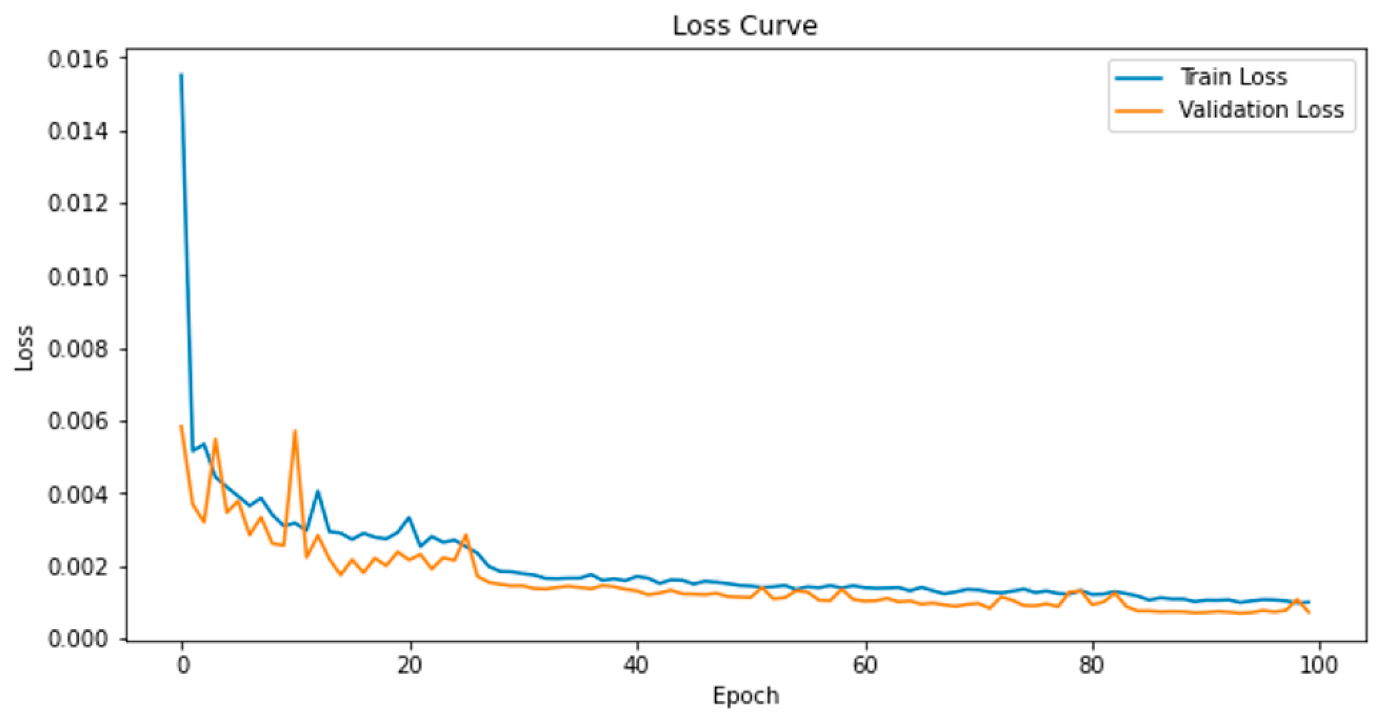
4.7. Model Performance Analysis

Given the diverse nature of network attack methods, corresponding defense strategies must be tailored accordingly. Traditional binary classification methods struggle to accurately identify specific attack types, making multi-class classification experiments necessary. These experiments enable a more granular categorization of intrusion detection data, enhancing the precision of attack recognition and defense strategies.

Figure 13, Figure 14, and Figure 15 illustrate the training loss curves of DIMK-GCN on the CIC-IDS2017, CIC-IDS2018, and Edge-IIoTSet datasets, respectively. As shown in the loss curves, at the beginning of training, both training and validation losses decrease at a similar rate without significant divergence, indicating that the model performs well on training data while maintaining strong generalization capability, thereby reducing the risk of overfitting. On the Edge-IIoTSet dataset, the model rapidly learns feature representations during the early training phase, with both training and validation losses decreasing simultaneously, demonstrating good generalization. As training progresses, the rate of loss reduction slows, accompanied by slight fluctuations, but the overall generalization ability remains stable. In the later stages, the loss stabilizes, suggesting that the model has converged effectively, achieving high fitting accuracy while maintaining robust generalization performance.

Results in

Table 6. CIC-IDS2017 results by attack type (%).

Label Type	Evaluation Indicators
	ACC	Recall	F1
BENIGN	99.55	99.57	99.56
DoS Hulk	97.83	99.29	98.56
PortScan	99.34	99.93	99.65
DDoS	99.82	99.85	99.88
DoS GoldenEye	99.43	98.88	99.17
FTP-Patator	99.17	97.98	98.57
SSH-Patator	99.53	99.03	99.12
DoS slowloris	98.62	98.79	98.71
DoS Slowhttptest	92.30	98.09	95.11
Web Attack -Brute Force	96.72	94.21	94.25
Web Attack -XSS	93.22	96.85	96.87
Infiltration	94.36	95.89	95.82
Web Attack -Sql Injection	92.23	93.56	93.54
Heartbleed	93.15	94.21	94.23

and

Table 7. CIC-IDS2018 results by attack type (%).

Label Type	Evaluation Indicators
	ACC	Recall	F1
Benign	99.68	99.63	99.62
DDOS attack-HOIC	99.12	99.18	99.18
DoS attacks-Hulk	99.26	99.10	99.20
Bot	99.63	99.40	99.42
FTP-BruteForce	98.61	96.71	97.43
SSH-Bruteforce	98.17	98.72	98.97
Infilteration	98.23	98.32	98.35
DoS attacks-SlowHTTPTest	98.72	98.94	98.95
DoS attacks-GoldenEye	97.20	97.59	97.61
DoS attacks-Slowloris	96.83	96.92	96.92
DDOS attack-LOIC-UDP	93.12	93.81	93.83
Brute Force -Web	94.42	95.10	95.12
Brute Force -XSS	92.23	93.56	93.54
SQL Injection	91.85	91.93	91.93

demonstrate that the model achieved excellent performance for most attack types, particularly PortScan, DDoS, SSH-Patator, DDOS attack-HOIC, DoS attacks-Hulk, and Bot. However, the model exhibited some underperformance for certain specific attack types.

The classification results of DIMK-GCN for different attack types are shown in and 7. The results indicate that the model achieves excellent performance on most attack types, particularly in identifying PortScan, DDoS, SSH-Patator, DDOS attack-HOIC, DoS attacks-Hulk, and Bot attacks with high accuracy. However, certain attack types exhibit a degree of underreporting. The detection rate for web attacks (XSS/SQL injection) is primarily limited by the imbalanced distribution of data categories. Although the SMOTE oversampling technique was applied to balance class distribution, the original dataset contained very few XSS/SQL injection samples (less than 0.3%), making it difficult for the model to fully capture their feature space. Additionally, these attack features exhibit high overlap with normal traffic, and the synthetic samples generated by oversampling may introduce noise, further reducing the model’s generalization ability for small sample categories.

As shown in

Table 8. CIC-IDS2018 results by attack type (%).

Label Type	Evaluation Indicators
	ACC	Recall	F1
Normal	99.21	99.32	99.32
DOS/DDOS	96.06	97.10	97.10
Information gathering	98.13	97.11	96.50
Injection attacks	97.35	97.22	96.82
MITM	95.21	94.82	94.82
Malware attacks	97.21	96.12	95.89

, the model demonstrates strong overall performance on the Edge-IIoTSet dataset. For normal traffic, DoS/DDoS, information gathering, and injection attacks, the accuracy, recall, and F1-score remain consistently high, indicating the model’s effectiveness in detecting these attack types. Although the detection metrics for MITM and malware attacks are relatively lower, the overall detection performance remains robust without significant imbalance. These results suggest that the model exhibits strong resilience in identifying various attack types. Future work can focus on optimizing the detection of attack types with slightly lower performance to further enhance overall effectiveness.

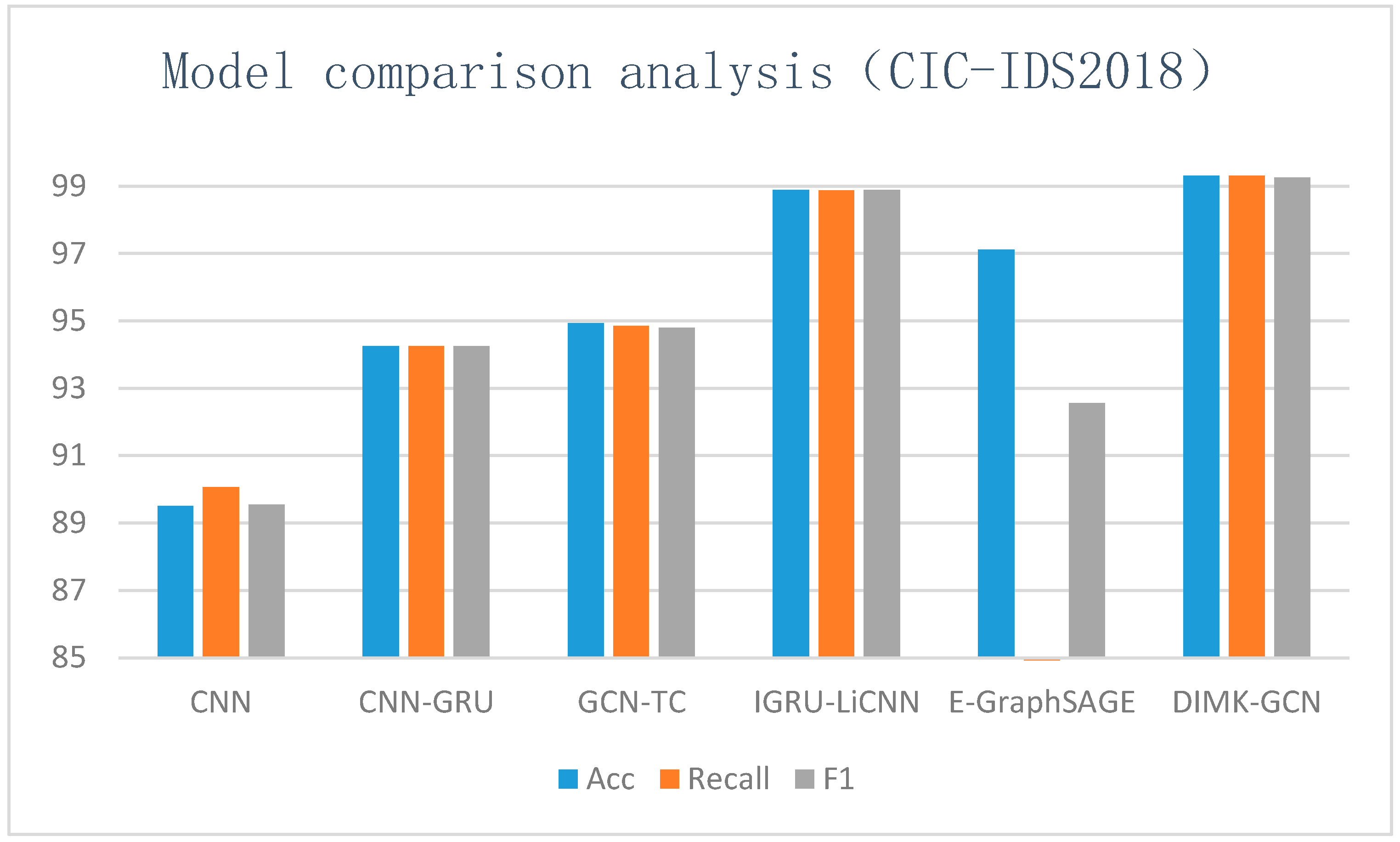
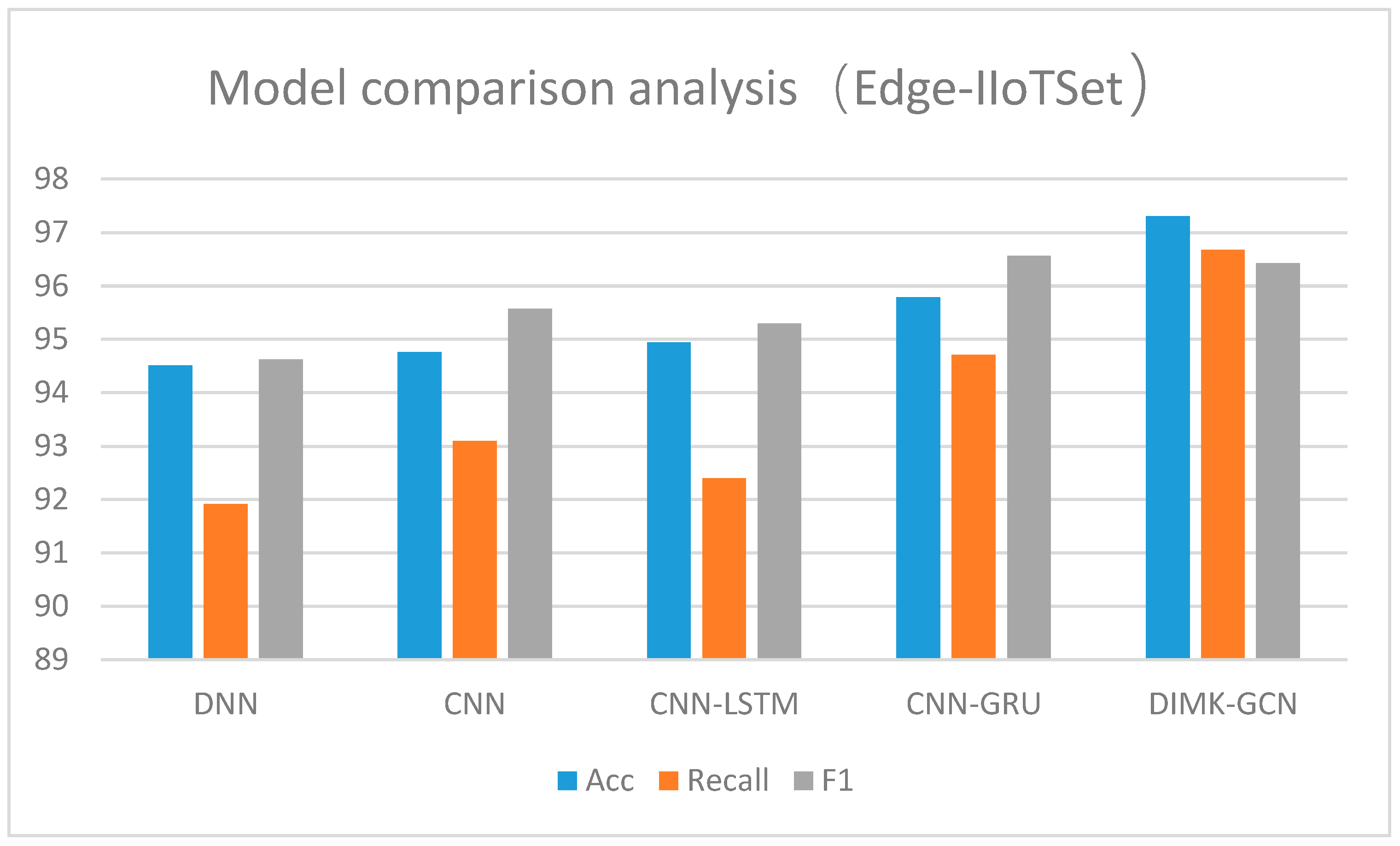
4.8. Comparative Analysis

To ensure the objectivity and reliability of this study, four representative models were selected for comparison: CNN-GRU [27], GCN-TC [28], E-GraphSAGE [29], and IGRU-LiCNN [5]. CNN-GRU combines CNN for spatial feature extraction with GRU to capture long-range dependencies, and an attention mechanism is applied to weight key features, enhancing their representation capability. GCN-TC leverages GCN to learn hidden representations of network traffic data and utilizes the local homogeneity of graphs to construct an IP connection-based graph structure, thereby uncovering potential attack behaviors. E-GraphSAGE extends the application of graph neural networks in intrusion detection by not only modeling edge features of traffic records but also incorporating an improved GraphSAGE sampling and aggregation strategy for dynamic modeling of both local and global patterns. IGRU-LiCNN focuses on lightweight design, integrating GRU with an optimized CNN structure to improve the efficiency of spatiotemporal feature extraction. It further enhances feature weight allocation through a channel attention mechanism, enabling efficient detection. The final model comparison results are shown in Figure 16 and Figure 17.

As shown in the results, the DIMK-GCN model outperforms other models in terms of accuracy, a significant advantage attributed to its multi-kernel graph convolution and temporal fusion mechanisms. These mechanisms enable DIMK-GCN to effectively capture and analyze the complex graph structure and temporal characteristics of network traffic. In contrast, CNN and its variants exhibit relatively lower accuracy due to their limited capability in exploring graph structures. Although GCN-TC performs well in graph convolution, DIMK-GCN achieves superior performance through a more optimized combination of graph convolution and temporal information fusion. While IGRU-LiCNN and E-GraphSAGE also demonstrate high accuracy, they fall short of DIMK-GCN due to the lack of deeper feature fusion and attention enhancement.

As shown in Figure 18, the comparative experimental results on the Edge-IIoTSet dataset indicate that DIMK-GCN outperforms other models in overall performance, particularly in terms of accuracy and recall, demonstrating superior detection capability. Compared to traditional DNN and CNN models, DIMK-GCN leverages multi-channel graph convolution and dynamic interaction mechanisms to enhance feature learning and improve robustness against various attack types. Furthermore, compared to deep learning methods that incorporate temporal modeling, such as CNN-LSTM and CNN-GRU, DIMK-GCN maintains a stable F1-score, highlighting its superior ability to capture complex attack patterns.

5. Conclusions

The DIMK-GCN model proposed in this paper provides a new solution for network intrusion detection by innovatively integrating dynamic graph feature extraction and temporal information modeling, achieving excellent performance in key metrics such as accuracy. The strength of the DIMK-GCN model lies in applying the concept of multi-channel graph convolution and temporal feature iterative fusion to network intrusion detection, overcoming the limitations of traditional methods in feature extraction and temporal modeling. The proposed dynamic graph feature extraction mechanism offers a novel approach to representing complex network behaviors.

This model can be applied in the future to social network analysis for identifying anomalous community behaviors and predicting influence propagation paths. In recommendation systems, it can be used to model user interest drift and cross-domain recommendations to improve personalized recommendation effectiveness. In traffic flow prediction, the model is expected to combine road network topology with traffic fluctuation characteristics, enhancing the ability to learn congestion propagation patterns, thus providing theoretical support for dynamic traffic scheduling.

We acknowledge that the model still has limitations in detecting minority class attacks. Affected by data imbalance, the model’s recognition accuracy for minority classes needs improvement. Additionally, the graph construction method based on cosine similarity is limited in dynamic environments, as it only focuses on directional similarity and overlooks changes in feature magnitudes, making it difficult to effectively distinguish sudden traffic patterns. The fixed time window calculation also reduces its adaptability to rapidly changing traffic. Future research could optimize data balancing strategies and introduce a time-decaying dynamic weighting mechanism to make the graph structure more adaptive, thereby accurately capturing spatiotemporal correlations. Additionally, incorporating transformer-based spatiotemporal attention mechanisms would improve dynamic traffic modeling capabilities and enhance key feature extraction performance.

References

1. Ren, K.; Yuan, S.; Zhang, C.; Shi, Y.; Huang, Z. CANET: A hierarchical cnn-attention model for network intrusion detection. Comput. Commun. 2023, 205, 170–181. [Google Scholar]
2. Qazi, E.U.; Faheem, M.H.; Zia, T. HDLNIDS: Hybrid deep-learning-based network intrusion detection system. Appl. Sci. 2023, 13, 4921. [Google Scholar] [CrossRef]
3. Liu, G.; Zhang, J. CNID: Research of network intrusion detection based on convolutional neural network. Discret. Dyn. Nat. Soc. 2020, 2020, 4705982. [Google Scholar]
4. Xu, H.; Sun, L.; Fan, G.; Li, W.; Kuang, G. A hierarchical intrusion detection model combining multiple deep learning models with attention mechanism. IEEE Access 2023, 11, 66212–66226. [Google Scholar]
5. Zhou, C.; Yang, D.; Wei, S.J. Lightweight Network Intrusion Detection Model Integrating GRU and CNN. Comput. Syst. Appl. 2023, 32, 162–170. [Google Scholar]
6. Mittal, K.; Khurana Batra, P. Graph-ensemble fusion for enhanced IoT intrusion detection: Leveraging GCN and deep learning. Clust. Comput. 2024, 27, 10525–10552. [Google Scholar]
7. Lin, L.; Zhong, Q.; Qiu, J.; Liang, Z. E-GRACL: An IoT intrusion detection system based on graph neural networks. J. Supercomput. 2025, 81, 42. [Google Scholar]
8. Jahin, M.A.; Soudeep, S.; Mridha, M.F.; Kabir, R.; Islam, M.R.; Watanobe, Y. CAGN-GAT Fusion: A Hybrid Contrastive Attentive Graph Neural Network for Network Intrusion Detection. arXiv 2025, arXiv:2503.00961. [Google Scholar]
9. Tran, D.H.; Park, M. FN-GNN: A novel graph embedding approach for enhancing graph neural networks in network intrusion detection systems. Appl. Sci. 2024, 14, 6932. [Google Scholar] [CrossRef]
10. Abdullayeva, F.; Suleymanzade, S. Cyber security attack recognition on cloud computing networks based on graph convolutional neural network and graphsage models. Results Control Optim. 2024, 15, 100423. [Google Scholar] [CrossRef]
11. Nowroozi, E.; Taheri, R.; Hajizadeh, M.; Bauschert, T. Verifying the Robustness of Machine Learning based Intrusion Detection Against Adversarial Perturbation. In Proceedings of the 2024 IEEE International Conference on Cyber Security and Resilience (CSR), IEEE, London, UK, 2–4 September 2024; pp. 9–15. [Google Scholar]
12. Shojafar, M.; Taheri, R.; Pooranian, Z.; Javidan, R.; Miri, A.; Jararweh, Y. Automatic clustering of attacks in intrusion detection systems. In Proceedings of the 2019 IEEE/ACS 16th International Conference on Computer Systems and Applications (AICCSA), IEEE, Abu Dhabi, United Arab Emirates, 3–7 November 2019; pp. 1–8. [Google Scholar]
13. Reka, R.; Karthick, R.; Ram, R.S.; Singh, G. Multi head self-attention gated graph convolutional network based multi-attack intrusion detection in MANET. Comput. Secur. 2024, 136, 103526. [Google Scholar] [CrossRef]
14. Altaf, T.; Wang, X.; Ni, W.; Liu, R.P.; Braun, R. NE-GConv: A lightweight node edge graph convolutional network for intrusion detection. Comput. Secur. 2023, 130, 103285. [Google Scholar] [CrossRef]
15. Wang, Y.; Jiang, Y.; Lan, J. Intrusion detection using few-shot learning based on triplet graph convolutional network. J. Web Eng. 2021, 20, 1527–1552. [Google Scholar]
16. Veličković, P.; Cucurull, G.; Casanova, A.; Romero, A.; Lio, P.; Bengio, Y. Graph attention networks. arXiv 2017, arXiv:1710.10903. [Google Scholar]
17. Kipf, T.N.; Welling, M. Semi-supervised classification with graph convolutional networks. arXiv 2016, arXiv:1609.02907. [Google Scholar]
18. Cho, K. Learning phrase representations using RNN encoder-decoder for statistical machine translation. arXiv 2014, arXiv:1406.1078. [Google Scholar]
19. Shang, R.; Ma, Y. Electric Vehicle Charging Load Forecasting Based on K-Means++-GRU-KSVR. World Electr. Veh. J. 2024, 15, 582. [Google Scholar] [CrossRef]
20. Sharafaldin, I.; Lashkari, A.H.; Ghorbani, A.A. Toward generating a new intrusion detection dataset and intrusion traffic characterization. ICISSp 2018, 1, 108–116. [Google Scholar]
21. Leevy, J.L.; Khoshgoftaar, T.M. A survey and analysis of intrusion detection models based on cse-cic-ids2018 big data. J. Big Data 2020, 7, 1–19. [Google Scholar] [CrossRef]
22. Ferrag, M.A.; Friha, O.; Hamouda, D.; Maglaras, L.; Janicke, H. Edge-IIoTset: A new comprehensive realistic cyber security dataset of IoT and IIoT applications for centralized and federated learning. IEEE Access 2022, 10, 40281–40306. [Google Scholar] [CrossRef]
23. Lanvin, M.; Gimenez, P.F.; Han, Y.; Majorczyk, F.; Mé, L.; Totel, É. Errors in the CICIDS2017 dataset and the significant differences in detection performances it makes. In Proceedings of the International Conference on Risks and Security of Internet and Systems, Sousse, Tunisia, 7–9 December 2022; Springer Nature: Cham, Switzerland, 2022; pp. 18–33. [Google Scholar]
24. Liu, L.; Engelen, G.; Lynar, T.; Essam, D.; Joosen, W. Error prevalence in nids datasets: A case study on cic-ids-2017 and cse-cic-ids-2018. In Proceedings of the 2022 IEEE Conference on Communications and Network Security (CNS), IEEE, Virtually, 3–5 October 2022; pp. 254–262. [Google Scholar]
25. Mohammadian, H.; Ghorbani, A.A.; Lashkari, A.H. A gradient-based approach for adversarial attack on deep learning-based network intrusion detection systems. Appl. Soft Comput. 2023, 137, 110173. [Google Scholar]
26. Idrissi, M.J.; Alami, H.; El Mahdaouy, A.; El Mekki, A.; Oualil, S.; Yartaoui, Z.; Berrada, I. Fed-anids: Federated learning for anomaly-based network intrusion detection systems. Expert Syst. Appl. 2023, 234, 121000. [Google Scholar]
27. Cao, B.; Li, C.; Song, Y.; Qin, Y.; Chen, C. Network intrusion detection model based on CNN and GRU. Appl. Sci. 2022, 12, 4184. [Google Scholar] [CrossRef]
28. Zheng, J.; Li, D. GCN-TC: Combining trace graph with statistical features for network traffic classification. In Proceedings of the ICC 2019-2019 IEEE International Conference on Communications (ICC), IEEE, Shanghai, China, 20–24 May 2019; pp. 1–6. [Google Scholar]
29. Lo, W.W.; Layeghy, S.; Sarhan, M.; Gallagher, M.; Portmann, M. E-graphsage: A graph neural network based intrusion detection system for iot. In Proceedings of the NOMS 2022-2022 IEEE/IFIP Network Operations and Management Symposium, IEEE, Budapest, Hungary, 25–29 April 2022; pp. 1–9. [Google Scholar]
Figure 1. DIMK-GCN overall framework.
Electronics 14 01391 g001
Figure 2. GAT structure diagram.
Electronics 14 01391 g002
Figure 3. GCN structure diagram.
Electronics 14 01391 g003
Figure 4. GRU structure diagram.
Electronics 14 01391 g004
Figure 5. Spatiotemporal feature weighting module.
Electronics 14 01391 g005
Figure 6. CIC-IDS2017 top 20 features.
Electronics 14 01391 g006
Figure 7. CIC-IDS2018 top 20 features.
Electronics 14 01391 g007
Figure 8. Interactive graph feature fusion module.
Electronics 14 01391 g008
Figure 9. Temporal feature learning module.
Electronics 14 01391 g009
Figure 10. Ablation experiment results.
Electronics 14 01391 g010
Figure 11. Number of channels and accuracy.
Electronics 14 01391 g011
Figure 12. Number of channels and F1-score.
Electronics 14 01391 g012
Figure 13. Model loss convergence curve (CIC-IDS2017).
Electronics 14 01391 g013
Figure 14. Model loss convergence curve (CIC-IDS2018).
Electronics 14 01391 g014
Figure 15. Model loss convergence curve (Edge-IIoTSet).
Electronics 14 01391 g015
Figure 16. Model comparison analysis (CIC-IDS2017).
Electronics 14 01391 g016
Figure 17. Model comparison analysis (CIC-IDS2018).
Electronics 14 01391 g017
Figure 18. Model comparison analysis (Edge-IioTSet).
Electronics 14 01391 g018