Recursive PID-NT Estimation-Based Second-Order SMC Strategy for Knee Exoskeleton Robots: A Focus on Uncertainty Mitigation

Abstract

This study introduces a modified second-order super-twisting sliding mode control algorithm designed to enhance the precision and robustness of knee exoskeleton robots by incorporating advanced uncertainty mitigation techniques. The key contribution of this research is the development of an efficient estimation mechanism capable of accurately identifying model parameter uncertainties and patients’ unwanted action torques disturbance within a finite time horizon, thereby improving overall system performance. The proposed control framework ensures smooth and precise control signal dynamics while effectively suppressing chattering effects, a common drawback in conventional sliding mode control methodologies. The theoretical foundation of the algorithm is rigorously established through the formulation of a PID non-singular terminal sliding variable, which ensures finite time stability in the sliding phase and a comprehensive Lyapunov-based stability analysis assuming that the upper bound of the uncertainty and its derivative are known in the reaching phase, which collectively guarantee the system’s robustness and reliability. Through simulations, the efficacy of the proposed control system is evaluated in its ability to track diverse desired knee angles, demonstrate robustness against disturbances, such as those caused by the patient’s foot reaction, and handle a 20% uncertainty in the model parameters. Additionally, the system’s effectiveness is assessed by three individuals with varying parameters. Notably, the controller gains remain consistent across all scenarios. This research constitutes a significant advancement in the domain of knee exoskeleton control, offering a more reliable and precise methodology for addressing model uncertainties.

1. Introduction

Exoskeleton systems, designed to mitigate injury risks and enhance physical endurance, are particularly beneficial for individuals engaged in physically demanding tasks. These lightweight structures are engineered for comfort and provide an extensive range of motion. Minimizing unnecessary complexity and simplifying control mechanisms ensures increased reliability and ease of use. Recent advancements in robotic technology have driven significant interest in orthotic and exoskeleton systems. These robotic assistive devices have emerged as a promising solution for augmenting human biomechanics, delivering substantial benefits in rehabilitation, injury prevention, and performance enhancement [1,2].

Knee exoskeletons are used in rehabilitation to aid recovery from injuries and neurological conditions, assist mobility-impaired individuals with daily activities, reduce fatigue and injury risk in industrial tasks, enhance performance and prevent injuries in sports and fitness, and augment soldiers’ strength and endurance in military operations [3,4].

In recent years, significant advancements have been made in exoskeleton hardware and software, further enhancing their potential applications [5]. Innovations such as artificial intelligence (AI)-powered simulation training have improved human performance in robotic exoskeletons, while new designs like robotic hip exoskeletons show promise for aiding stroke patients. Additionally, the development of lightweight, energy-efficient actuators and advanced materials has led to more comfortable and effective exoskeletons. These advancements underscore the growing importance of exoskeletons in various fields, from medical rehabilitation to industrial applications, and highlight the need for continued research and development to address existing challenges and expand their capabilities [6].

The knee joint is essential in facilitating the transition. Consequently, the meticulous design and precise control of a powered knee exoskeleton are pivotal for the success of lifting tasks [7]. Thanks to revolutionary advancements in multidisciplinary fields like mechatronics and computing, realistic exoskeleton devices are now a reality [8]. However, exoskeleton systems often encounter challenges arising from nonlinear dynamics, unmodeled behaviors, and external disturbances. Addressing these uncertainties is crucial to ensure consistent and reliable performance [9]. To address uncertainty in knee exoskeletons, several strategies are proposed such as implementing sensors that can accurately detect and respond to changes in terrain and user movement [10], using machine learning to predict and mitigate uncertainties based on user data and environmental factors [11], providing comprehensive training to ensure users can effectively adapt to and utilize the exoskeleton [12], and implementing control algorithms which can manage uncertainties and improve the exoskeleton’s response to varying conditions.

To ensure accurate tracking and control, various algorithms have been proposed, including the Proportional–Derivative (PD) controller [13]. However, linear controllers often face limitations in their effectiveness, confined to a specific operational range around the system’s nominal point. Additionally, the dynamics of human–robot interaction forces complicate control strategies, as these forces are interwoven with actuator control inputs, presenting a challenge for effective control. Alternative strategies, such as the intelligent neural network compensation control approach referenced in [14], necessitate a lengthy training process and an assessment of a dynamic model, as mentioned in [15]. A method for controlling uncertain systems is to employ disturbance observer-based control. In particular, control mechanisms utilizing an extended state observer are capable of simultaneously estimating both the unknown state variable and the uncertainties [9].

Sliding mode control (SMC) has become a notable solution for its robustness against uncertainties and disturbances [16]. Previous studies have effectively employed SMCs in regulating knee exoskeletons [17,18]. However, traditional SMC methods suffer from ‘chattering’, a high-frequency oscillation in the control signal that can cause instability [19]. This is attributed to the discontinuous sign function present in standard SMC laws. To overcome traditional SMC limitations, various approximation methods like saturation or tanh functions have been introduced [20]. In [21], a combination of SMC and backstepping method is utilized for controller design. In this approach, system disturbances are estimated using a nonlinear observer. However, the standard SMC is employed, and to eliminate chattering, an approximated function is used instead of the sign function. Yet, these often sacrifice tracking precision and system robustness, leading to sliding paths deviating from the intended surface.

A promising alternative, high-order SMC (HOSMC), strives to reduce both the sliding variable and its derivatives to zero. However, implementing HOSMC poses practical challenges due to the requirement for higher-order derivatives of the sliding variable. In contrast, the second-order super-twisting (ST) SMC offers a viable solution as it requires only the sliding variable [22,23]. However, the ST control signal is not completely smooth.

Observer-based SMC (OB-SMC) can be utilized to estimate disturbances, leading to a reduction in chattering amplitude and enhanced disturbance rejection capabilities [24,25]. Although previous studies have employed observers to estimate uncertainties in knee exoskeleton control [26], controlling the chattering continues to be a significant challenge. Some observer-based methods have substituted the sign function with continuous functions to mitigate chattering [27]. However, replacing the sign function with any continuous function for chattering elimination and signal smoothing inevitably leads to a reduction in accuracy. Additionally, demonstrating the stability of the closed-loop system and synchronizing the bandwidths of the observer and controller present significant challenges that are frequently disregarded in observer-based controllers.

In [28], an SMC that utilizes a linear extended state observer has been introduced for knee exoskeleton robots. A notable limitation of this method is the absence of guaranteed finite-time stability, particularly in the sliding phase. This is attributed to the dependence on a linear combination of tracking error and its derivatives to define the sliding variable. Typically, conventional SMC utilizes a linear relation based on error and its derivatives to define the sliding surface. As an alternative, designing a Proportional–Integral (PI) sliding variable that incorporates the integral of the error can enhance the performance of the closed-loop system, owing to its contribution to steady-state tracking [29]. However, both approaches only guarantee asymptotic stability, meaning errors, but never truly reach zero [30]. This limitation can affect performance in high-precision applications.

To attain finite-time stability during the sliding phase, terminal SMC (T-SMC) uses a nonlinear function in the sliding variable. While this allows for finite-time convergence, it may lead to a singularity issue [31]. This limitation can be addressed by employing non-singular terminal SMC (NT-SMC), which guarantees finite-time convergence without the problem of singularity [32]. Additionally, the PI non-singular terminal sliding surface combines the benefits of PI and NT-SMC, integrating the tracking error for steady-state error elimination and offering robust tracking performance with finite-time stability.

In conclusion, the control challenges in the field of SMC design for knee exoskeleton robots can be summarized as follows:

Chattering in standard SMC: Methods based on standard SMC face the fundamental challenge of chattering, rendering their application impractical. Additionally, methods relying on continuous approximation experience a decrease in accuracy.

Observer-based methods stability: Observer-based methods must ensure the closed-loop system’s stability. Consequently, the stability of the controller and the observer cannot be considered in isolation.

Finite-time stability: Employing the conventional sliding variable, which relies on a linear combination of tracking error and its derivatives, does not ensure finite-time stability in the sliding mode. Additionally, it does not guarantee that the overall system stability will be in the form of finite-time variety.

Convergence time in SOSMC: Although approximation methods may affect system performance, second-order SMC (SOSMC) is promising in attaining smoother control signals. Nonetheless, challenges persist in ensuring finite-time stability and convergence time.

This paper addresses key challenges by introducing a knee exoskeleton model and designing an innovative disturbance cancellation-based recursive Proportional–Integral–Derivative (PID) non-singular terminal SOSMC. This advanced controller integrates sliding variable and uncertainty estimation variables to ensure precise knee joint angle tracking while delivering a chattering-free control signal via a modified super-twisting SOSMC reaching law. The proposed method uses a compensatory term to eliminate uncertainty effects based on estimation, and therefore, this method has more calculations and complexity compared to the standard method in exchange for eliminating chattering. The non-singular terminal sliding variable guarantees finite-time stability in the sliding phase, and a simple Lyapunov analysis confirms the finite-time stability of the closed-loop system.

The paper is structured as follows: Section 2 provides a detailed examination of the dynamic model of the knee exoskeleton, which includes an analysis of system parameters and uncertainties. Section 3 delineates the novel uncertainty cancellation-based recursive PID non-singular terminal SOSMC. Section 4 provides simulation results and performance comparisons of the proposed controller. Finally, Section 5 synthesises the findings and offers concluding remarks for the paper.

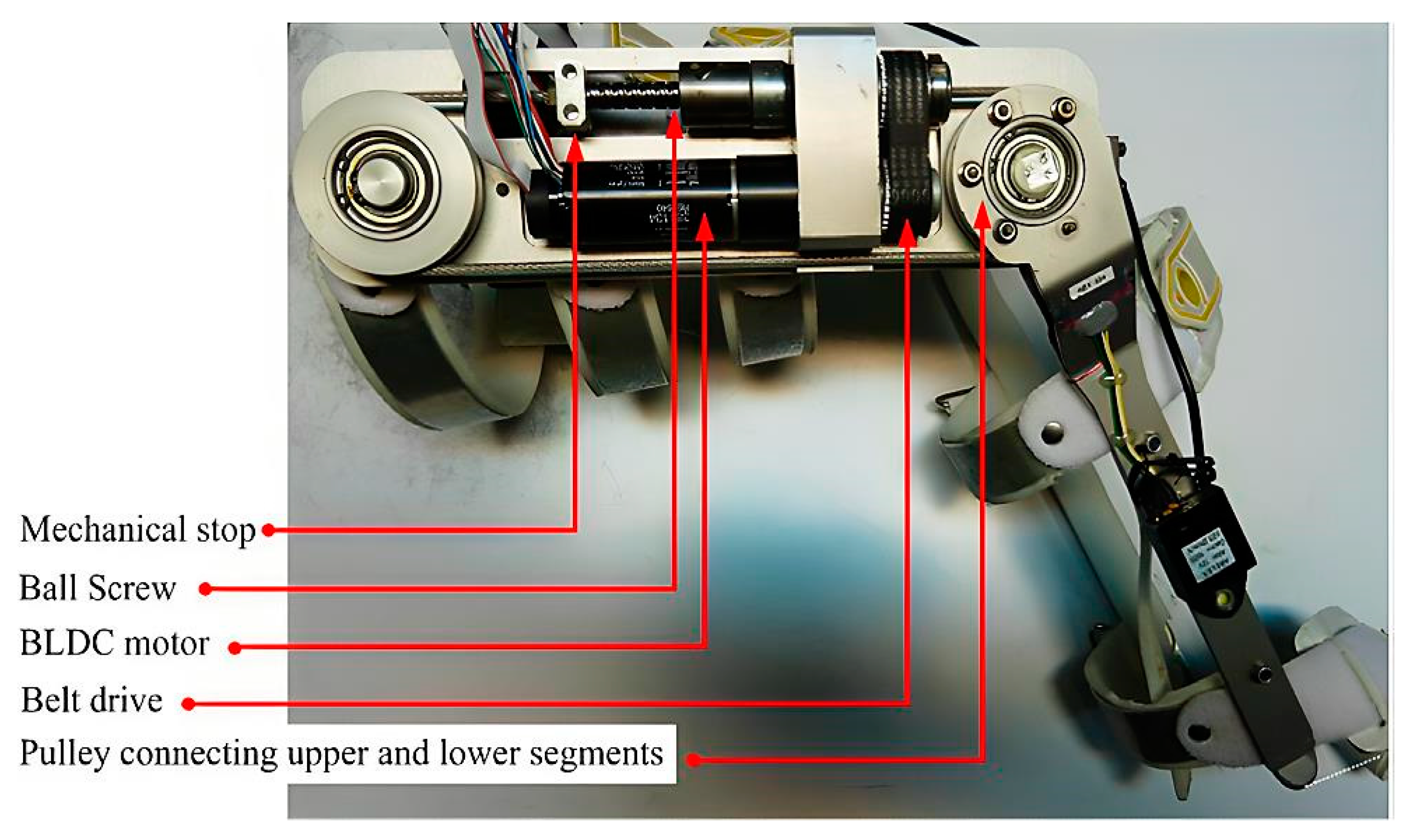
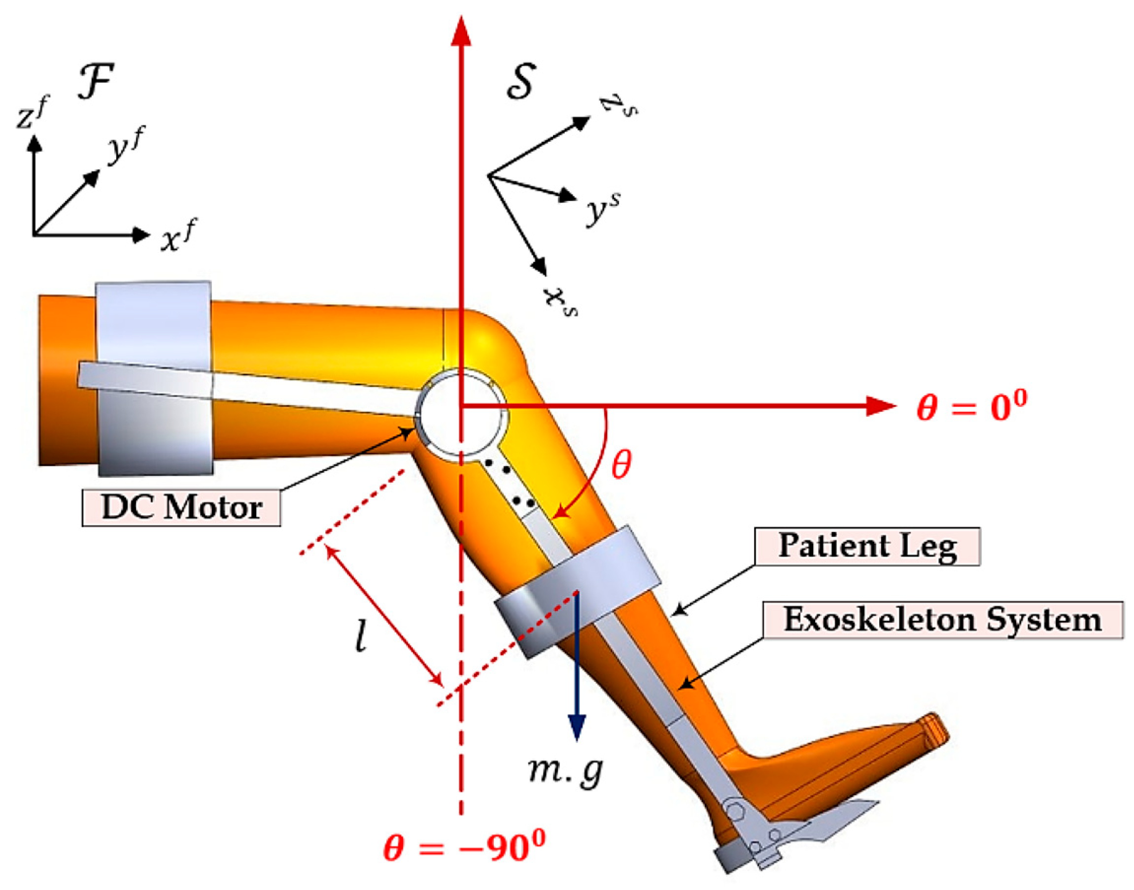
2. Modeling of Exoskeleton Dynamics

For precise control of knee exoskeletons, such as knee position control robots, it is essential to develop an accurate dynamic model that has been thoroughly validated through testing [33].

Figure 1 illustrates the orthosis, comprising two segments attached to the thigh and shank. It articulates around a singular rotational degree of freedom (DOF) at the knee joint and is secured to the wearer’s leg with suitable braces. The knee joint’s single DOF is actuated by both an external actuator and the user’s thigh muscles.

The dynamic model of the knee exoskeleton system is formulated as follows [34]:

$$J\ddot{\theta }=-{\tau }_{g}cos\theta -Asign\dot{\theta }-B\dot{\theta }-K\left(\theta -{\theta }_r\right)+{\tau }_e+{\tau }_h$$

(1)

where $J=J_s+J_o$ is the inertia of the shank and orthosis; ${\tau }_g=m_s{l}_{s}g+m_o{l}_{o}g$ is the gravitational torque in which $m_i$ and $l_i (i\in \{s,o\})$ are the masses and lengths of the shank and orthosis, respectively; the parameters $A=A_s+A_o$ and $B=B_s+B_o$ represent the solid and viscous friction parameters, respectively; $K$ denotes the stiffness of the knee joint; ${\theta }_r$ indicates the resting position of the knee joint; and ${\tau }_e$ and ${\tau }_h$ are the input torques from the actuator and human effort, respectively. Figure 2 includes the upper part (thigh) and the lower part (leg) along with the foot and shank frames. The articulation range of the exoskeleton encompasses a spectrum from 0 to −135 wherein 0° represents the angle of total extension of the knee joint, −90° corresponds to the knee joint’s rest position, and −135° denotes the angle of maximal flexion for the knee joint.

The external disturbance (patient’s unwanted action torques) and uncertainties of the parameters are the control challenges of this study. To solve this challenge, it is essential to first identify all uncertainties and disturbances affecting the system. The dynamic model, as presented in Equation (1), is reformulated as Equation (2) to incorporate these uncertainties [21].

$$\begin{array}{c}\left(J+∆J\right)\ddot{\theta }=-\left({\tau }_g+∆{\tau }_g\right)cos\theta -\left(A+∆A\right)sign\dot{\theta }-\left(B+∆B\right)\dot{\theta }\\ -\left(K+∆K\right)\left(\theta -{\theta }_r\right)+{\tau }_e+{\tau }_h\end{array}$$

(2)

The parameter uncertainties mentioned above arise from variations in characteristics such as inertia, masses, and lengths of the shank and orthosis, as well as solid and viscous friction parameters and the stiffness of the knee joint. Consequently, the total uncertainties are calculated as follows:

$$d={\displaystyle \frac{{\tau }_h-∆J\ddot{\theta }-∆{\tau }_{g}cos\theta -∆Asign\dot{\theta }-∆B\dot{\theta }-∆K\left(\theta -{\theta }_r\right)}{J}}$$

(3)

For modeling, we consider the state variables as $x_1=\theta \mathrm{a}\mathrm{n}\mathrm{d} x_2=\dot{\theta }$. Additionally, the control input is considered as $u={\tau }_e$. As a result, Equation (2) becomes the following state equation:

$$\dot{x}=f\left(x\right)+g_1\left(x\right)u+g_2\left(x\right)d$$

(4)

where $x=\left[\begin{array}{c}\theta \\ \dot{\theta }\end{array}\right]$, $f\left(x\right)=\left[\begin{array}{c}{x}_2\\ {\displaystyle \frac{-{\tau }_{g}cos\theta -Asign\dot{\theta }-B\dot{\theta }-K\left(\theta -{\theta }_r\right)}{J}}\end{array}\right]$, $g_1\left(x\right)=\left[\begin{array}{c}0\\ {\displaystyle \frac{1}{J}}\end{array}\right]$, and $g_2\left(x\right)=\left[\begin{array}{c}0\\ 1\end{array}\right]$. The parameters of the model include $A$, $B$, $K$, ${\tau }_g$, and $J$. Two effective factors for measuring the ${\tau }_g$ and $J$ parameters are the human shank and orthosis. Therefore, these two parameters consist of $J_s$ and ${\tau }_s$, which are related to the human shank, and $J_o$ and ${\tau }_o$, which are related to orthosis. $J_s$ and ${\tau }_s$ can be calculated by the weight and height of the subject [18]. ${\tau }_o$ and $J_o$ can be obtained by using a nonlinear least squares optimization of Equation (1) [36]. The remaining parameters are determined through the passive pendulum test [34]. The parameter values are listed in

Table 1. Shank parameters.

Parameters	Value	Unit
$J=(J_s+J_o)$	0.326	$\mathrm{k}\mathrm{g}·{\mathrm{m}}^2$
${\tau }_g=({\tau }_{gs}+{\tau }_{go})$	15.341	$\mathrm{N}·\mathrm{m}$
K	0.114	$\mathrm{m}·\mathrm{r}\mathrm{a}{\mathrm{d}}^{-1}$
B	0.064	$\mathrm{N}·\mathrm{m}$
A	0.354	$\mathrm{N}·\mathrm{m}·\mathrm{s}·\mathrm{r}\mathrm{a}{\mathrm{d}}^{-1}$

.

The open-loop system response to a 5 Nm torque input is depicted in Figure 3a,b. It is observable that while the joint angle remains stable at steady state, it exhibits oscillatory behavior with significant overshoot during the transient state, indicating the necessity for closed-loop control of the system. Furthermore, when introducing disturbances from foot reactions and a 20% uncertainty in model parameters, as shown in Figure 3c,d, the output accuracy is severely compromised by these disturbances and uncertainties, resulting in suboptimal behavior at steady state.

3. Main Results

The control objective in this paper is to ensure that the output from Equation (4) conforms to the predetermined trajectory via the application of the control law. This is crucial, given the potential external disturbances and the model’s uncertainties. Furthermore, this section includes a comprehensive stability analysis.

3.1. Mathematical Foundation

Consider the uncertain nonlinear system as follows:

$$\left\{\begin{array}{c}\dot{x}=p\left(x\right)+g\left(x\right)u+d\left(t\right) \\ y=l\left(x\right) \end{array}\right.$$

(5)

where $x\in X\subset R^n$ is the state variable vector, $u\in \mathbb{R}$ and $y\in \mathbb{R}$ are the control input and system output, respectively, and $p(x)$, $g(x)$, and $l(x)$ are nonlinear functions. The term $d(t)$ denotes the collective sum of uncertainties, which includes the dynamics not captured by the model, errors in determining parameters, and any external perturbations.

The performance of closed-loop systems is significantly influenced by the choice of sliding variables in SMC. The sliding surfaces presented subsequently are defined for a second-order system and $ϵ=y-y_d$, in which $y$ is the system’s output and $y_d$ is the system’s desired trajectory.

Definition 1.

The conventional sliding variable is defined for a second-order system based on the dynamics of error as follows:

$${\sigma }_C=\dot{ϵ}+{\tau }_Cϵ$$

(6)

The parameter $c$ represents the time constant at which the error decays exponentially to zero when the system is in sliding phase ${\sigma }_C=0$. It can be deduced that, for ${\tau }_C>0$ , the derivation of the tracking error is exponentially stable.

Remark 1.

Referring to Equation (6), the sliding variable derivative is determined to be the following:

$${\dot{\sigma }}_C=\ddot{ϵ}+{\tau }_C\dot{ϵ}$$

(7)

Consequently, based on Equation (7), the characteristic polynomial is derived as follows:

$$S^2+{\tau }_{c}S=0$$

(8)

As a result, during the sliding phase, a particular eigenvalue of the system is invariant. Adherence to the Hurwitz criterion ensures that certain closed-loop system behaviors are inherently stable and cannot be altered through tuning.

Definition 2.

A sliding surface can be presented based on PID form, crafted to boost the system’s tracking capabilities within the structure of SMC. The integration of an integral term of the error into the sliding variable is intended to potentially enhance the precision of tracking, particularly in the boundary layer. This leads to the creation of a PID-based sliding surface SMC as follows [37]:

$${\sigma }_P={\tau }_d\dot{ϵ}+{\tau }_pϵ+{\tau }_i{\int }_{t_0}^tϵdt$$

(9)

Remark 2.

Using Equation (9), the sliding surface derivative is the following:

$$\dot{{\sigma }_P}={\tau }_d\ddot{ϵ}+{\tau }_p\dot{ϵ}+{\tau }_iϵ$$

(10)

According to Equation (17), the characteristic polynomial equation will be derived as follows:

$${\tau }_d{S}^2+{\tau }_{p}S+{\tau }_i=0$$

(11)

where ${\tau }_d$, ${\tau }_p$, and ${\tau }_i$ are selected in accordance with Equation (11). This selection is made to strictly fulfil the Hurwitz criterion, which is essential for system stability. As a result, the tracking error during the sliding phase is guaranteed to be exponentially stable. Additionally, by altering the values of ${\tau }_d$, ${\tau }_p$, and ${\tau }_i$, it is possible to adjust both eigenvalues of the system. This grants full flexibility in modifying the system’s behavior.

Definition 3.

Terminal SMC incorporates a nonlinear element into the sliding surface, effectively turning it into a point of attraction. This alteration stabilizes the system within a definite period, presenting a benefit by achieving stability faster compared to the gradual stability provided by conventional SMC. A recognized terminal sliding variable, denoted, is established in the following manner [30]:

$${\sigma }_T=\dot{ϵ}+{\tau }_T{\left|ϵ\right|}^{\gamma }sign\left(ϵ\right)$$

(12)

with $\tau \mathit{>}0$, and 0 <$\gamma$< 1.

Remark 3.

When employing T-SMC, the system trajectories reach the sliding surface defined by ${\sigma }_T=0$ less than a certain time. Subsequently, the tracking error is also expected to diminish to zero within a finite time of sliding. Nevertheless, due to the presence of the non-singular terms, the control signal escalates towards infinity.

Definition 4.

To enhance control measures and tackle the singularity challenges that are prevalent in conventional terminal SMC (T-SMC) approaches, the non-singular terminal SMC (NT-SMC) method has been developed [38]. This technique guarantees the finite-time convergence of the tracking error throughout the sliding phase, despite the presence of uncertain model or system parameters, intrinsic nonlinearities, and external interferences. The non-singular terminal sliding variable is established as follows:

$${\sigma }_N=ϵ+{\displaystyle \frac{1}{{\tau }_N}}{\left|\dot{ϵ}\right|}^{\gamma }sign\left(\dot{ϵ}\right)$$

(13)

Remark 4.

Applying the NT-SMC strategy ensures that the trajectories of the system will converge to the sliding surface (${\sigma }_N=0$) in finite time. Subsequently, it is guaranteed that the tracking error will converge to zero within a predetermined sliding period. Crucially, it guarantees the control signal remains continuous and non-singular.

Definition 5.

Consider the nonlinear system of Equation (5) and variable $\sigma$, and the following set:

$$\mathsf{\Sigma }=\{\mathrm{x}\in \mathrm{X}|\mathsf{\sigma }(\mathrm{x},\mathrm{t})=0\}$$

(14)

called the ‘sliding variable’. When $\mathsf{\sigma }$ reaches zero, the system of Equation (5) will exhibit a favorable dynamic behavior.

In practical applications, achieving an ‘ideal’ sliding mode, as outlined in Definition 5, is not feasible. Therefore, introducing the concept of a ‘real’ sliding mode becomes essential.

Definition 6.

Following [39], and considering $\sigma (x, t)$, the “real sliding variable” is as follows (with $\xi$ > 0):

$${\mathsf{\Sigma }}^{\mathrm{*}}=\left\{\mathrm{x}\in \mathrm{X}\right|\left|\sigma \right|<\xi \}$$

(15)

Definition 7.

Consider the real sliding variable ${\Sigma }^{*}$as defined by Equation (15). The behavior of the system of Equation (5) when constrained by Equation (15) is termed the ‘real sliding mode’. The dynamics of the sliding variable are as follows:

$$\dot{\sigma }={\displaystyle \frac{\partial \sigma }{\partial t}}+{\displaystyle \frac{\partial \sigma }{\partial x}}p\left(x\right)+{\displaystyle \frac{\partial \sigma }{\partial x}}g\left(x\right)u+h\left(t\right)=a\left(x,t\right)+b\left(x,t\right)u+h\left(t\right)$$

(16)

where $a\left(x,t\right)$ and $b\left(x,t\right)$ are nonlinear known functions and $h(t)$ is the uncertain term. Considering the nonlinear system characterized by uncertainty as presented in Equation (5), and the dynamics of the sliding variable $\mathsf{\sigma }(\mathrm{x},\mathrm{t})$ outlined in Equation (16), the system is regulated by a comprehensive control law:

$$u={\displaystyle \frac{-a(x,t)+u_{sw}}{b(x,t)}}$$

(17)

where $u_{sw}$ is the switching control and can be determined based on SMC theories. In standard SMC the switching term is designed as follows:

$$u_{sw}=-\eta sign\left(\sigma \right)$$

(18)

where $\eta$ is the reaching term.

Remark 5.

Using the conventional SMC of Equation (10) leads to $\dot{\sigma }=h(t)-\eta sign(\sigma )$ where with gain $\eta ={\eta }^{*}+\mu$ and for $\left|h(t)\right|<{\eta }^{*}$ we have $\mu \le {\displaystyle \frac{\sigma (0)}{t_r}}$, and $t_r$ is reaching time.

Lemma 1.

The dynamic equation

$$\dot{\sigma }=-\eta {\left|\sigma \right|}^{\gamma }sign\left(\sigma \right)$$

(19)

for $\eta >0$ and $0>\gamma >1$ is finite-time stable with $t_r\le {\displaystyle \frac{{\sigma (0)}^{1-\gamma }}{{\eta }_2(1-\gamma )}}$.

Remark 6.

In Equation (19), which represents a nominal system devoid of uncertainty, finite-time stability is assured, and chattering is absent. However, in the presence of uncertainty $h\left(t\right)$ within Equation (19), to ensure robustness, a term analogous to Equation (18) must be incorporated into this relationship as follows:

$$\dot{\sigma }=-{\eta }_1{\left|\sigma \right|}^{\gamma }sign\left(\sigma \right)-{\eta }_{2}sign\left(\sigma \right)+h\left(t\right)$$

(20)

To mitigate chattering, the super-twisting theory is used as shown in Equation (21):

$$\left\{\begin{array}{l}\dot{\sigma }=-{\eta }_1{\left|\sigma \right|}^{{\displaystyle \frac{1}{2}}}sign(\sigma )+z\\ \dot{z}=-{\eta }_{2}sign\left(\sigma \right)+\dot{h}\left(t\right)\end{array}\right.$$

(21)

where $z={\eta }_2\int sign\left(\sigma \right)d\tau +h\left(t\right)$. This control law is unable to produce a complete smooth control signal. Therefore, a smooth SOSMC has be introduced in the following manner [40]:

$$\left\{\begin{array}{l}{u}_{sw}=-z_1-{\eta }_1{\left|\sigma \right|}^{{\displaystyle \frac{m}{\left(m+1\right)}}}sign(\sigma )+w\\ \dot{w}=-{\eta }_2{\left|\sigma \right|}^{{\displaystyle \frac{\left(m-1\right)}{\left(m+1\right)}}}sign(\sigma )\end{array}\right.$$

(22)

with ${\eta }_1,{\eta }_2>0$ and $m\ge 1$.

Remark 7.

Variable $z_1$ represents an estimate obtained by an observer. In control theory, an observer is a system that provides estimates of the internal states or disturbances of a dynamic system based on its outputs. Specifically, it estimates the uncertainties and external disturbances affecting the system. In this context, the observer is used to estimate the unknown or uncertain terms that influence the system’s behavior, such as $h(t)$. This estimated value $z_1$ is then used in the control law to improve system performance and ensure stability. The stability of this theory can be guaranteed based on the principle of homogeneous systems [40].

Definition 8.

A function $f(x)$ is positive definite, if and only if the following obtain:

I 

For every non-zero vector $x$, $f\left(x\right)>0$;

II 

For zero vector $x$, $f\left(x\right)=0$;

III 

$f\left(x\right)=x^{T}Ax$ for a symmetric matrix $A$.

Lemma 2.

Note that

$$\left|x_1\right|\left(\left|x_2\right|+\left|x_3\right|\right)\ge x_1\left(x_2+x_3\right)$$

(23)

Lemma 3.

Take into account the well-known inequality

$$\left|x_1\right|+\left|x_2\right|\ge \left|x_1+x_2\right|$$

(24)

Lemma 4.

Following [41], to guarantee finite-time convergence of a nonlinear system $\dot{x}=f(x)$, the following condition must be established$:$

$$\dot{V}<-Q$$

(25)

where $V\left(x\right)>0$ is the Lyapunov function and $Q$ is a positive constant.

3.2. Proposed Rescursive PID NT Estimation-Based SOSMC

In this section, we introduce a two-part design for the proposed controller. Initially, to ensure finite-time stability during the sliding phase, we select an appropriate sliding variable. Subsequently, for the reaching phase, we aim to achieve finite-time convergence while enhancing robustness against uncertainties and generating a smooth control signal. This is accomplished by incrementally refining the conventional SMC to derive a conductive component. Moreover, the finite-time stability in the arrival phase is substantiated using the Lyapunov method.

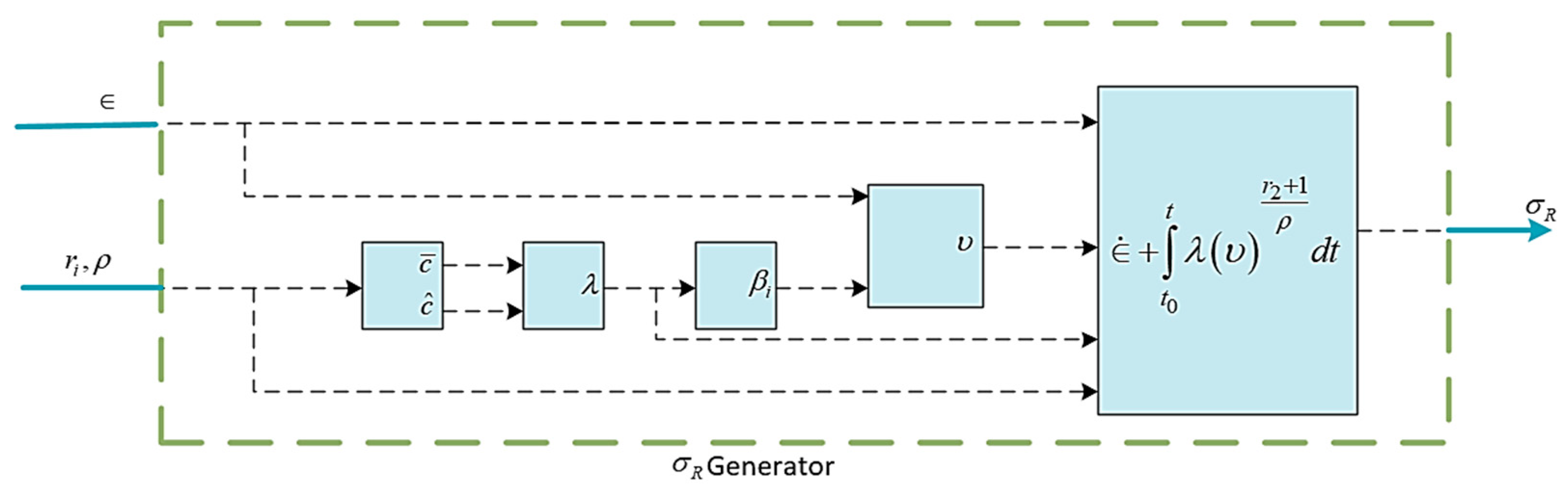
3.2.1. Sliding Variable Design

It has been observed that the majority of non-singular TSM control methods are limited to solving control design issues for a specific type of second-order uncertain nonlinear systems. Consequently, a significant amount of research has focused on adapting these second-order non-singular TSM controls for application to higher-order systems. The recursive non-singular terminal SMC offers adequate conditions for stability within a finite time frame by employing an innovative approach to fractional power design. The sliding surface structure is presented as follows [42]:

$$\begin{array}{c}{\sigma }_R=\dot{ϵ}+{\int }_{t_0}^t\lambda {(v}^{{\displaystyle \frac{r_2+1}{\rho }}})dt\\ \upsilon \left(t\right)={\beta }_1{ϵ}^{{\displaystyle \frac{\rho }{r_1}}}+{\beta }_2{\dot{ϵ}}^{{\displaystyle \frac{\rho }{r_2}}}\end{array}$$

(26)

with $r_i>0$ and for $i\in \mathbb{N}$, $\rho >{max}_{i\in \mathbb{N}}\left\{r_i\right\}$ and

$${\beta }_1={\lambda }^{{\displaystyle \frac{\rho }{r_1+1}}} , {\beta }_2=1$$

(27)

$$\lambda =\overline{c}+\widehat{c}+L$$

(28)

$$\overline{c}={\displaystyle \frac{r_2}{\mu 2^{\frac{r_2}{\rho }}}}{\left({\displaystyle \frac{\left(2\mu -r_2\right)2^{2-\frac{r_2}{\rho } }}{\mu L}}\right)}^{{\displaystyle \frac{2\mu (2\mu -r_2)}{\rho r_2}}}$$

(29)

$$\widehat{c}={\displaystyle \frac{L}{8}}$$

(30)

in which $L$ and $\mu$ are constant gains.

Remark 8.

With this approach, the power factors $\rho$, $r_1$, and $r_2$ can be set in advance to guarantee the closed-loop system stability in a finite time frame. Figure 4 demonstrates the correlation of gains for the formation of ${\sigma }_R$ in the recursive PID non-singular TSMC approach.

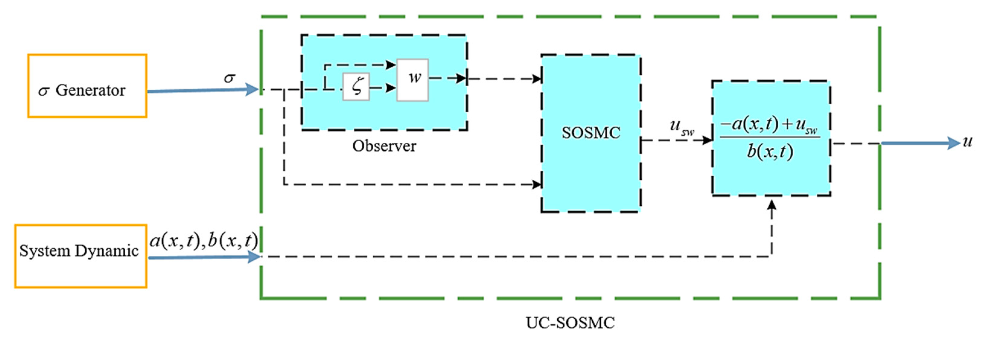
3.2.2. Reaching Controller Design

The reaching controller proposed represents a systematic enhancement over the conventional SMC approach, incorporating necessary modifications to fulfill the control objectives of this article. The primary goal is to establish a smooth, robust nonlinear controller that ensures finite-time convergence of the closed-loop system during both the reaching and sliding phases. To secure finite-time convergence in the sliding phase, the recursive PID non-singular terminal sliding variable from Equation (26) will be utilized. The attainment of finite-time-reaching control is also detailed within this section.

In the initial step, we examine the proposed switching controller, which is predicated on the standard SMC methodology, as delineated below:

$$u_{sw}=-{\eta }_{1}sign\left(\sigma \right)$$

(31)

By using this controller, the sliding variable dynamics will be $\dot{\sigma }=-{\eta }_{1}sign\left(\sigma \right)+h(t)$ and it is evident that the finite-time stability of the sliding variable is attainable by selecting the ${\eta }_1$ gain to be larger than the upper limit of uncertainty $h(t)$. In this control law, the direct inclusion of the sign function causes chattering. To solve this problem, we modify the controller from Equation (31) as follows:

$$u_{sw}=-{\eta }_1{\left|\sigma \right|}^{{\gamma }_1}sign\left(\sigma \right)$$

(32)

where $0<{\gamma }_1<1$, and using Equation (32), the sliding variable dynamic is the following:

$$\dot{\sigma }=-{\eta }_1{\left|\sigma \right|}^{{\gamma }_1}sign\left(\sigma \right)+h\left(t\right)$$

(33)

Considering Equation (33), it is determined when $0<\sigma <1$, for $0<{\gamma }_1<1$ the term ${\eta }_1{\left|\sigma \right|}^{{\gamma }_1}$ is less than $h(t)$. Therefore, the controller will not be capable of countering the system’s uncertainties. To remedy this limitation, we can incorporate the estimation of the uncertain component (w) into Equation (33) as follows:

$$u_{sw}=-{\eta }_1{\left|\sigma \right|}^{{\gamma }_1}sign\left(\sigma \right)+w$$

(34)

Considering $z=w+h(t)$, the sliding variable dynamics will be as follows:

$$\left\{\begin{array}{c}\dot{\sigma }=-{\eta }_1{\left|\sigma \right|}^{{\gamma }_1}sign\left(\sigma \right)+z\\ \dot{z}=\dot{w}+\dot{h}(t) \end{array}\right.$$

(35)

From $\dot{z}=\dot{w}+\dot{h}(t)$, a suitable choice for $\dot{w}$ to ensure robust stabilization of $z$ is $\dot{w}=-{\eta }_{2}sign\left(\sigma \right)$ that leads to $\dot{z}=-{\eta }_{2}sign\left(\sigma \right)+\dot{h}(t)$. Another choice to achieve smoother behavior in $\dot{w}$ is

$$\dot{w}=-{\eta }_2{\left|\sigma \right|}^{{\gamma }_2}sign\left(\sigma \right)$$

(36)

where $0<{\gamma }_2<1$, and considering $z=w+h(t)$, we obtain the following:

$$\left\{\begin{array}{c}\dot{\sigma }=-{\eta }_1{\left|\sigma \right|}^{{\gamma }_1}sign\left(\sigma \right)+z \\ \dot{z}=-{\eta }_2{\left|\sigma \right|}^{{\gamma }_2}sign\left(\sigma \right)+\dot{h}(t)\end{array}\right.$$

(37)

With this choice, the proposed controller will exhibit behavior akin to second-order SMC, thereby fulfilling one of the control objectives, namely, the generation of a smooth control signal. However, as previously noted, when $0<\sigma <1$, the term $-{\eta }_2{\left|\sigma \right|}^{{\gamma }_2}sign\left(\sigma \right)$ is insufficient to counteract the uncertainty $\dot{h}(t)$ in the dynamics of $z$. To resolve this, a robust term is introduced to $\dot{w}$ such that

$$\left\{\begin{array}{c}{u}_{sw}=-{\eta }_1{\left|\sigma \right|}^{{\gamma }_1}sign\left(\sigma \right)+w \\ \dot{w}=-{\eta }_2{\left|\sigma \right|}^{{\gamma }_2}sign\left(\sigma \right)+\chi \end{array}\right.$$

(38)

The term $\chi$ is introduced to enhance robustness against the uncertainty $\dot{h}(t)$ and its dynamics will be delineated through Lyapunov stability analysis in the subsequent theorem.

Theorem 1.

Given the nonlinear uncertain system of Equation (5) with the sliding variable $\sigma (x, t)$ as defined in Equation (26), and controlled by Equation (38), there exists a finite time $t_r>0$ such that a sliding mode is established for all $t \ge t_r$.

Proof. 

By employing the reaching control law delineated in Equation (38), and incorporating a straightforward robust term $\chi =-{\eta }_{3}sign\left(\mathsf{\Theta }\right)$, where $\mathsf{\Theta }$ is an updating term defined as $\mathsf{\Theta }=\sigma -\zeta$, the dynamics of the sliding variable are derived as follows:

$$\left\{\begin{array}{l}\dot{\sigma }=-{\eta }_1{\left|\sigma \right|}^{{\gamma }_1}sign\left(\sigma \right)+w+h(t) \\ \dot{w}=-{\eta }_2{\left|\sigma \right|}^{{\gamma }_2}sign\left(\sigma \right)-{\eta }_{3}sign\left(\mathsf{\Theta }\right)\\ \dot{\zeta }=f(\sigma ,w,\Theta ) \end{array}\right.$$

(39)

Let us contemplate the subsequent candidate for the Lyapunov function:

$$V={\displaystyle \frac{{\eta }_2}{1+{\gamma }_2}}{\left|\sigma \right|}^{1+{\gamma }_2}+{\displaystyle \frac{1}{2}}{\left(w+h\right)}^2+{\eta }_3\left|\mathsf{\Theta }\right|$$

(40)

This function is positive definite if ${\eta }_2,{\eta }_3>0$. When computing the time derivative of the function $V$ under the condition that $V\ne 0$, the following result is derived:

$$\dot{V}={\eta }_2{\left|\sigma \right|}^{{\gamma }_2}sign\left(\sigma \right)\dot{\sigma }+\left(w+h\right)\left(\dot{w}+\dot{h}\right)+{\eta }_{3}sign\left(\mathsf{\Theta }\right)\dot{\mathsf{\Theta }}$$

(41)

By incorporating Equation (39) into the above relationship, the derivative of V will take the following form:

$$\begin{array}{c}\dot{V}={\eta }_2{\left|\sigma \right|}^{{\gamma }_2}sign\left(\sigma \right)\left(-{\eta }_1{\left|\sigma \right|}^{{\gamma }_1}sign\left(\sigma \right)+\left(w+h\right)\right)\\ +\left(w+h\right)\left(-{\eta }_2{\left|\sigma \right|}^{{\gamma }_2}sign\left(\sigma \right)-{\eta }_{3}sign\left(\mathit{\Theta }\right)+\dot{h}\right)+{\eta }_{3}sign\left(\mathit{\Theta }\right)\dot{\mathit{\Theta }}\end{array}$$

(42)

Substituting $\dot{\mathsf{\Theta }}=\dot{\sigma }-\dot{\zeta }$ into Equation (42) yields the following:

$$\begin{array}{l}\dot{V}=-{\eta }_1{\eta }_2{\left|\sigma \right|}^{{\gamma }_1+{\gamma }_2}+{\eta }_2{\left|\sigma \right|}^{{\gamma }_2}sign\left(\sigma \right)\left(w+h\right)-{\eta }_2{\left|\sigma \right|}^{{\gamma }_2}sign\left(\sigma \right)\left(w+h\right)\\ \hspace{1em}\hspace{1em}\hspace{1em}-{\eta }_{3}sign\left(\mathit{\Theta }\right)\left(w+h\right)+\dot{h}\left(w+h\right)+{\eta }_{3}sign\left(\mathit{\Theta }\right)\left(\dot{\sigma }-f\left(\sigma ,w,\mathit{\Theta }\right)\right)\\ \hspace{1em}\hspace{1em}\hspace{1em}={\eta }_1{\eta }_2{\left|\sigma \right|}^{{\gamma }_1+{\gamma }_2}-{\eta }_{3}sign\left(\mathit{\Theta }\right)\left(w+h\right)+\dot{h}\left(w+h\right)\\ \hspace{1em}\hspace{1em}\hspace{1em}-{\eta }_1{\left|\sigma \right|}^{{\gamma }_1}sign\left(\sigma \right){\eta }_{3}sign\left(\mathit{\Theta }\right)+\left(w+h\left(t\right)\right){\eta }_{3}sign\left(\mathit{\Theta }\right)\\ \hspace{1em}\hspace{1em}\hspace{1em}-f\left(\sigma ,w,\mathit{\Theta }\right){\eta }_{3}sign\left(\mathit{\Theta }\right)\\ \hspace{1em}\hspace{1em}\hspace{1em}={\eta }_1{\eta }_2{\left|\sigma \right|}^{{\gamma }_1+{\gamma }_2}+\dot{h}\left(w+h\right)-{\eta }_1{\left|\sigma \right|}^{{\gamma }_1}sign\left(\sigma \right){\eta }_{3}sign\left(\mathit{\Theta }\right)\\ \hspace{1em}\hspace{1em}\hspace{1em}-f\left(\sigma ,w,\mathit{\Theta }\right){\eta }_{3}sign\left(\mathit{\Theta }\right).\end{array}$$

(43)

Considering $f(\sigma ,w,\mathit{\Theta })=-{\eta }_1{\left|\sigma \right|}^{{\gamma }_1}sign\left(\sigma \right)+{\displaystyle \frac{\delta \left(\left|w\right|+\rho \right)}{{\eta }_3}}sign\left(\mathit{\Theta }\right)+{\eta }_4\mathit{\Theta }$ and substituting it into Equation (43) yields the following:

$$\dot{V}=-{\eta }_1{\eta }_2{\left|\sigma \right|}^{{\gamma }_1+{\gamma }_2}+\dot{h}\left(w+h\right)-\delta \left(\left|w\right|+\rho \right)-{\eta }_3{\eta }_4\left|\mathsf{\Theta }\right|$$

(44)

where ${\eta }_4>0.$ By considering $q$, which is a positive constant, Equation (45) can be derived as follows:

$$\begin{array}{c}\dot{V}\le -{\eta }_1{\eta }_2{\left|\sigma \right|}^{{\gamma }_1+{\gamma }_2}+\dot{h}\left(w+h\right)-\delta \left(\left|w\right|+\left|h\left(t\right)\right|+q\right)-{\eta }_3{\eta }_4\left|\mathsf{\Theta }\right|=-{\eta }_1{\eta }_2{\left|\sigma \right|}^{{\gamma }_1+{\gamma }_2}\\ +\dot{h}\left(w+h\right)-\delta \left(\left|w\right|+\left|h(t)\right|\right)-\delta q-{\eta }_3{\eta }_4\left|\mathsf{\Theta }\right|\end{array}$$

(45)

In the following, we can deduce the following from Equation (45):

$$\begin{array}{l}\dot{V}\le -{\eta }_1{\eta }_2{\left|\sigma \right|}^{{\gamma }_1+{\gamma }_2}+\dot{h}\left(w+h\right)-\left(\left|\dot{h}\left(t\right)\right|+\mu \right)\left(\left|w\right|+\left|h\left(t\right)\right|\right)-\delta q-{\eta }_3{\eta }_4\left|\mathit{\Theta }\right|=\\ \hspace{1em}\hspace{1em}\hspace{1em}\hspace{1em}-{\eta }_1{\eta }_2{\left|\sigma \right|}^{{\gamma }_1+{\gamma }_2}+\dot{h}\left(w+h\right)-\left|\dot{h}\left(t\right)\right|\left(\left|w\right|+\left|h\left(t\right)\right|\right)-\mu \left|w\right|+\left|h\left(t\right)\right|-\delta q\\ \hspace{1em}\hspace{1em}\hspace{1em}\hspace{1em}-{\eta }_3{\eta }_4\left|\mathit{\Theta }\right|\end{array}$$

(46)

Considering Lemmas 2 and 3, we will have $\left|\dot{h}(t)\right|\left(\left|\mathrm{w}\right|+\left|h\right|\right)\ge \dot{h}\left(h+w\right)$ and $\left|w\right|+\left|h\right|\ge \left|w+h\right|$. Consequently, Equation (46) will take the following form:

$$\dot{V}\le -{\eta }_1{\eta }_2{\left|\sigma \right|}^{{\gamma }_1+{\gamma }_2}-\mu \left|h+w\right|-{\eta }_3{\eta }_4\left|\mathsf{\Theta }\right|-\delta q$$

(47)

For $\delta q=0$, we will obtain the following:

$$\dot{V}\le -{\eta }_1{\eta }_2{\left|\sigma \right|}^{{\gamma }_1+{\gamma }_2}-\mu \left|h+w\right|-{\eta }_3{\eta }_4\left|\mathsf{\Theta }\right|<0$$

(48)

Hence, $\dot{V}$ is negative throughout its domain, but for $\delta q>0$, we will obtain the following:

$$\dot{V}\le -{\eta }_1{\eta }_2{\left|\sigma \right|}^{{\gamma }_1+{\gamma }_2}-\mu \left|h+w\right|-{\eta }_3{\eta }_4\left|\mathsf{\Theta }\right|-\delta q<-\delta q$$

(49)

So, according to Lemma 4, the finite-time convergence of the system is guaranteed. Consequently, based on Lemma 1, Equation (49) indicates that the system converges in finite time. The convergence time is calculated as below:

$$t_r={\displaystyle \frac{V(0)}{\delta q}}$$

(50)

Finally, the proposed controller will be articulated in the form of the following equation:

$$\left\{\begin{array}{c}{u}_{sw}=-{\eta }_1{\left|\sigma \right|}^{{\gamma }_1}sign\left(\sigma \right)+w \\ \dot{w}=-{\eta }_2{\left|\sigma \right|}^{{\gamma }_2}sign\left(\sigma \right)-{\eta }_{3}sign\left(\mathsf{\Theta }\right) \\ \dot{\zeta }={\eta }_1{\left|\sigma \right|}^{{\gamma }_1}sign\left(\sigma \right)-{\displaystyle \frac{\delta \left(\left|w\right|+\rho \right)}{{\eta }_3}}sign\left(\mathsf{\Theta }\right)-{\eta }_4\left(\mathsf{\Theta }\right) \end{array}\right.$$

(51)

Under the conditions that ${\eta }_1,{\eta }_2,{\eta }_3,{\eta }_4>0$ and $0<{\gamma }_1,{\gamma }_2<1$, the stability of the system of Equation (5) is assured. Consequently, this leads to the variables $w$ and $\mathsf{\Theta }$ converging to $h(t)$ and $0$, respectively, within a finite period of time.□

Remark 9.

In the proposed method, the variable $\mathit{\Theta }$ serves as the updating variable, facilitating the convergence of w to the uncertainty $h(t)$. For $\mathit{\Theta }=\sigma -\zeta$, the methodology operates similarly to an estimation-based controller mentioned in Equation (51).

Consequently, the block diagram of the proposed uncertainty cancelation (UC) SOSMC reaching control is depicted as in Figure 5.

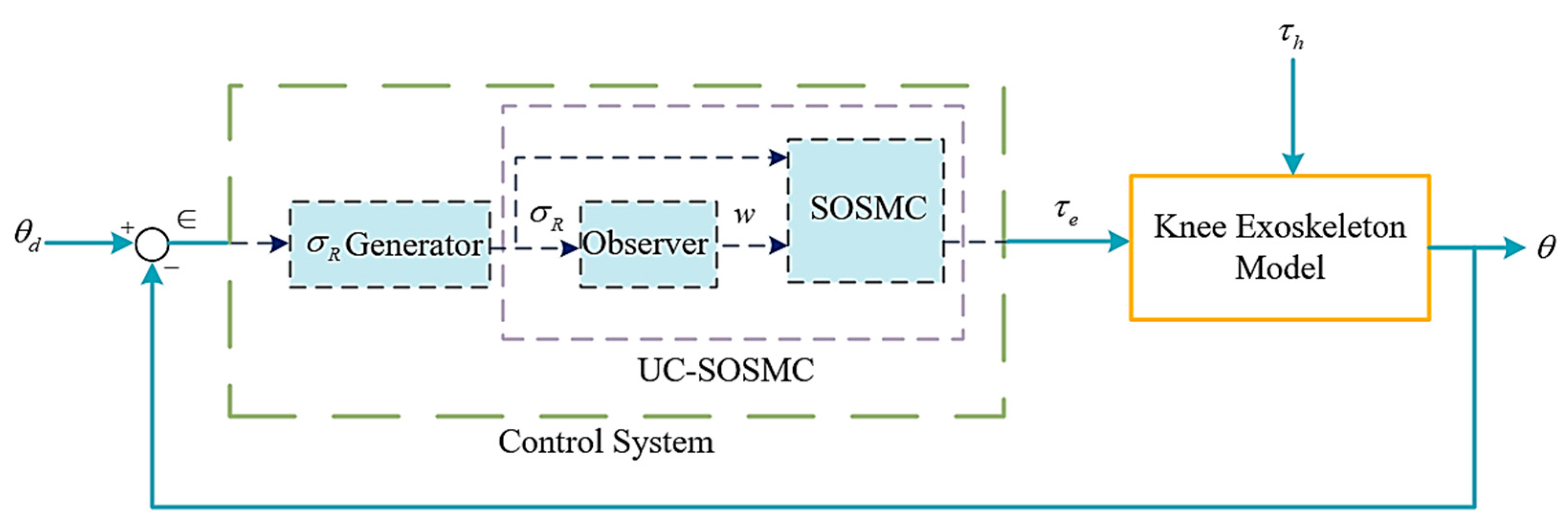
3.3. Knee Exoskeleton Control Using Proposed Controller

In this section, the proposed controller of Equation (51) is tailored for the knee exoskeleton framework. Given Equation (4), the objective is to align with the trajectory of $\theta$. To this end, we initially establish the system error in the ensuing manner:

$$ϵ=y-y_d=\theta -{\theta }_d$$

(52)

The recursive non-singular terminal sliding variable, predicated on the tracking error delineated in Equation (52) for the second-order nonlinear system represented by Equation (4), is defined as follows:

$$\begin{array}{c}{\sigma }_R=\dot{\theta }-{\dot{\theta }}_d+{\int }_{t_0}^t\lambda {\left(\upsilon \right)}^{{\displaystyle \frac{r_2+1}{\rho }}}dt\\ \upsilon \left(t\right)={\beta }_1{(\theta -{\theta }_d)}^{{\displaystyle \frac{\rho }{r_1}}}+{\beta }_2{(\dot{\theta }-{\dot{\theta }}_d)}^{{\displaystyle \frac{\rho }{r_2}}}\end{array}$$

(53)

The dynamic of the sliding variable from Equation (53) is governed by the subsequent computation:

$$\begin{array}{c}\dot{{\sigma }_R}=\ddot{ϵ}+\lambda {\left(\upsilon \right)}^{{\displaystyle \frac{r_n+1}{\rho }}} \\ ={\displaystyle \frac{1}{J}}\left(-{\tau }_{g}cos\theta -Asign\dot{\theta }-B\dot{\theta }-K\left(\theta -{\theta }_r\right)+{\tau }_e\right)-{\ddot{\theta }}_d+\lambda {\left(\upsilon \right)}^{{\displaystyle \frac{r_n+1}{\rho }}}\hfill \\ +{\displaystyle \frac{1}{J}}\left({\tau }_h-∆J\ddot{\theta }-∆{\tau }_{g}cos\theta -∆Asign\dot{\theta }-∆B\dot{\theta }-∆K\left(\theta -{\theta }_r\right)\right)\hfill \end{array}$$

(54)

in which

$$a\left(\theta ,\dot{\theta }\right)={\displaystyle \frac{1}{J}} \left(-{\tau }_{g}cos\theta -Asign\dot{\theta }-B\dot{\theta }-K\left(\theta -{\theta }_r\right)\right)-{\ddot{\theta }}_d+\lambda {\left(\upsilon \right)}^{{\displaystyle \frac{r_n+1}{\rho }}}$$

(55)

$$b\left(\theta ,\dot{\theta }\right)={\displaystyle \frac{1}{J}}$$

(56)

$$h\left(t\right)={\displaystyle \frac{1}{J}}\left({\tau }_h-∆J\ddot{\theta }-∆{\tau }_{g}cos\theta -∆Asign\dot{\theta }-∆B\dot{\theta }-∆K\left(\theta -{\theta }_r\right)\right)$$

(57)

The commanded torque ${\tau }_e$ for the knee exoskeleton is designed as follows:

$${\tau }_e={\tau }_{g}cos\theta +Asign\dot{\theta }+B\dot{\theta }+K\left(\theta -{\theta }_d\right)+J\left({\ddot{\theta }}_d+\lambda {\left(\upsilon \right)}^{{\displaystyle \frac{r_n+1}{\rho }}}+{{\tau }_e}_{sw}\right)$$

(58)

The proposed switching control input ${{\tau }_e}_{sw}$, derived through the recommended methodology, is formulated as follows:

$$\left\{\begin{array}{c}{{\tau }_e}_{sw}=-{\eta }_1{\left|{\sigma }_R\right|}^{{\gamma }_1}sign\left({\sigma }_R\right)+w \\ \dot{w}=-{\eta }_2{\left|\sigma \right|}^{{\gamma }_2}sign\left({\sigma }_R\right)-{\eta }_{3}sign\left({\sigma }_R-\zeta \right) \\ \dot{\zeta }={\eta }_1{\left|{\sigma }_R\right|}^{{\gamma }_1}sign\left({\sigma }_R\right)-{\displaystyle \frac{\delta \left(\left|w\right|+\rho \right)}{{\eta }_3}}sign\left({\sigma }_R-\zeta \right)-{\eta }_4\left({\sigma }_R-\zeta \right) \end{array}\right.$$

(59)

To assess stability, a positive definite Lyapunov function is established for the system as detailed below:

$$V_e={\displaystyle \frac{{\eta }_2}{1+{\gamma }_2}}{\left|{\sigma }_R\right|}^{1+{\gamma }_2}+{\displaystyle \frac{1}{2}}{\left(h+w\right)}^2+{\eta }_3\left|{\sigma }_R-\zeta \right|$$

(60)

$\dot{V_e}$ can be derived as follows:

$${\dot{V}}_e\le -{\eta }_1{\eta }_2{\left|{\sigma }_R\right|}^{{\gamma }_1+{\gamma }_2}-\mu \left|h+w\right|-{\eta }_3{\eta }_4\left|{\sigma }_R-\zeta \right|-\delta q<-\delta q$$

(61)

and convergence time is presented in the following form:

$$t_r={\displaystyle \frac{V_e(0)}{\delta q}}$$

(62)

Remark 10.

Using the proposed method, the torque required for the robot to track the desired angle in various scenarios is calculated based on Equations (58) and (59). These equations rely on variables such as the knee joint angle, angular velocity, and the nominal values of the robot and joint parameters, which must be measured using appropriate sensors. For implementation, an actuator, such as a BLDC motor (as shown in Figure 1), is needed to apply the torque command. During implementation, it is crucial to ensure proper coordination between the processor running the controller code, the sensor, and the actuator. If necessary, adjustments should be made to parameters such as the controller code’s discretization sample time.

4. Results

This section delineates the simulation results of the closed-loop system. The simulations were conducted using MATLAB 2024b. The knee exoskeleton’s performance is simulated within the Simulink environment, employing the equations delineated in Section 2. The proposed control system’s efficacy is assessed across diverse scenarios. Figure 6 presents the block diagram of the closed-loop system. In the proposed controller, the non-singular terminal sliding variable is initially computed from the knee angle tracking error. Subsequently, the system’s uncertainties, including parameter uncertainties and knee reflection torque, are estimated. The SOSMC then generates the control torque command based on the sliding variable, estimated uncertainties, and system dynamics.

In the first scenario, the performance of the proposed control system is evaluated in terms of its ability to track various desired knee angles. The second scenario examines the control system’s robustness against disturbances, such as those caused by the patient’s foot reaction, and a 20 percent uncertainty in the model parameters. The third scenario assesses the control system’s effectiveness for three individuals with varying parameters. Throughout all three scenarios, the controller gains are maintained as specified in

Table 2. List of controller gains.

Parameter	Value
${\eta }_1$	300
${\eta }_2$	20
${\eta }_3$	20
${\eta }_4$	10,000
${\gamma }_1$	0.9
${\gamma }_2$	0.3

. To ensure the Lyapunov function in Equation (60) is positive definite and its derivative in Equation (61) is negative definite, the parameters η₁ to η₄ must be positive. In Equation (59), η₁ directly influences the convergence of the sliding variable, η₂ aids the convergence of the W variable, and η₃ governs the updating term in W to address uncertainty. A larger η₃ can enhance the convergence speed of W to the uncertain function, while η₄ adjusts the convergence speed of the estimated sliding variable to the measured value. Thus, η₃ and η₄ should be tuned together to optimize the estimated variables.

In simulations, these parameters were fine-tuned through trial and error to handle various operating conditions, such as different desired inputs, parameter uncertainties, and disturbances, without requiring parameter changes across scenarios. Additionally, γ₁ and γ₂ were selected to control the smoothness of the control signal; smaller values yield faster responses but less smooth signals, whereas values closer to one produce smoother signals.

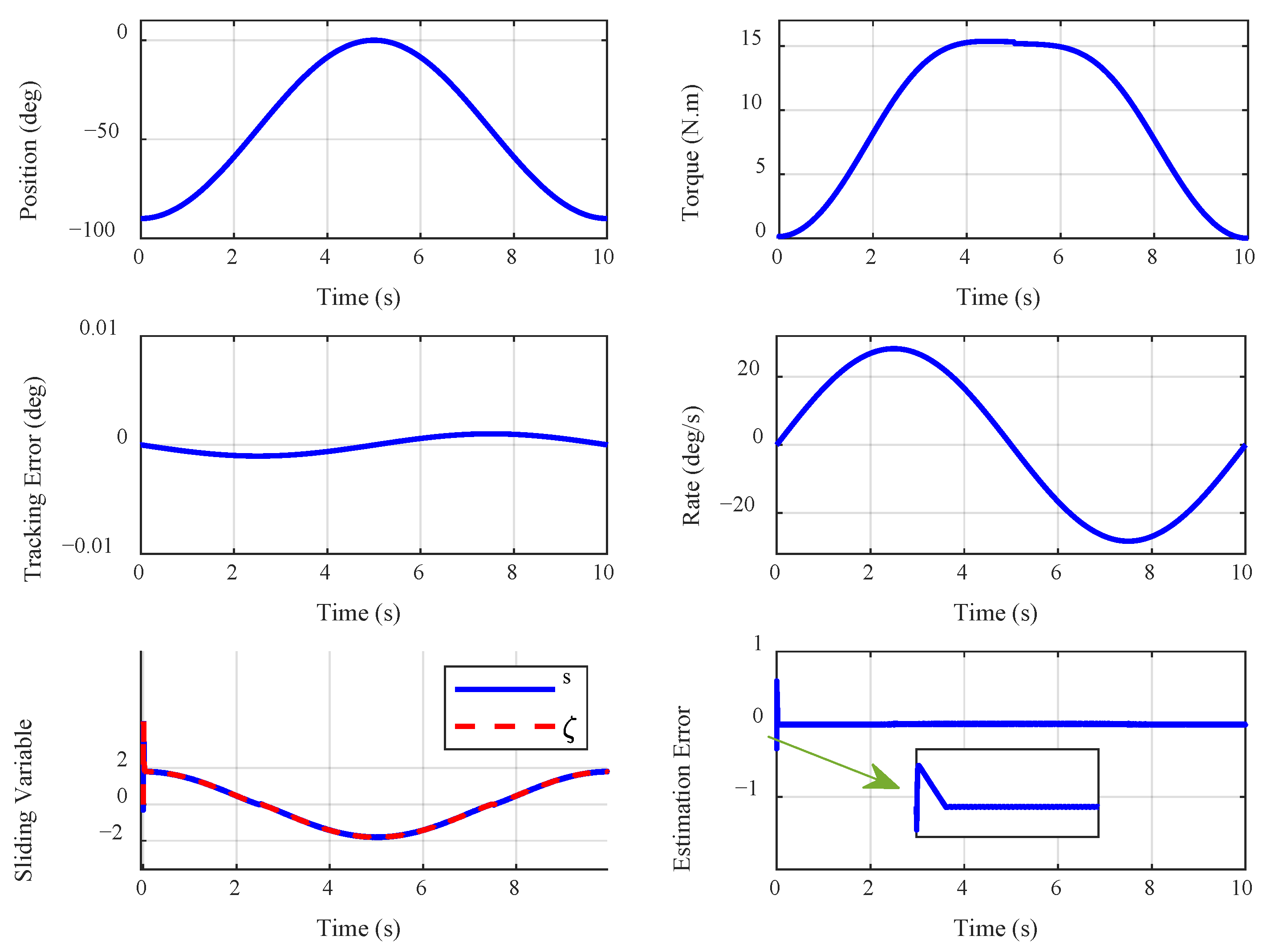
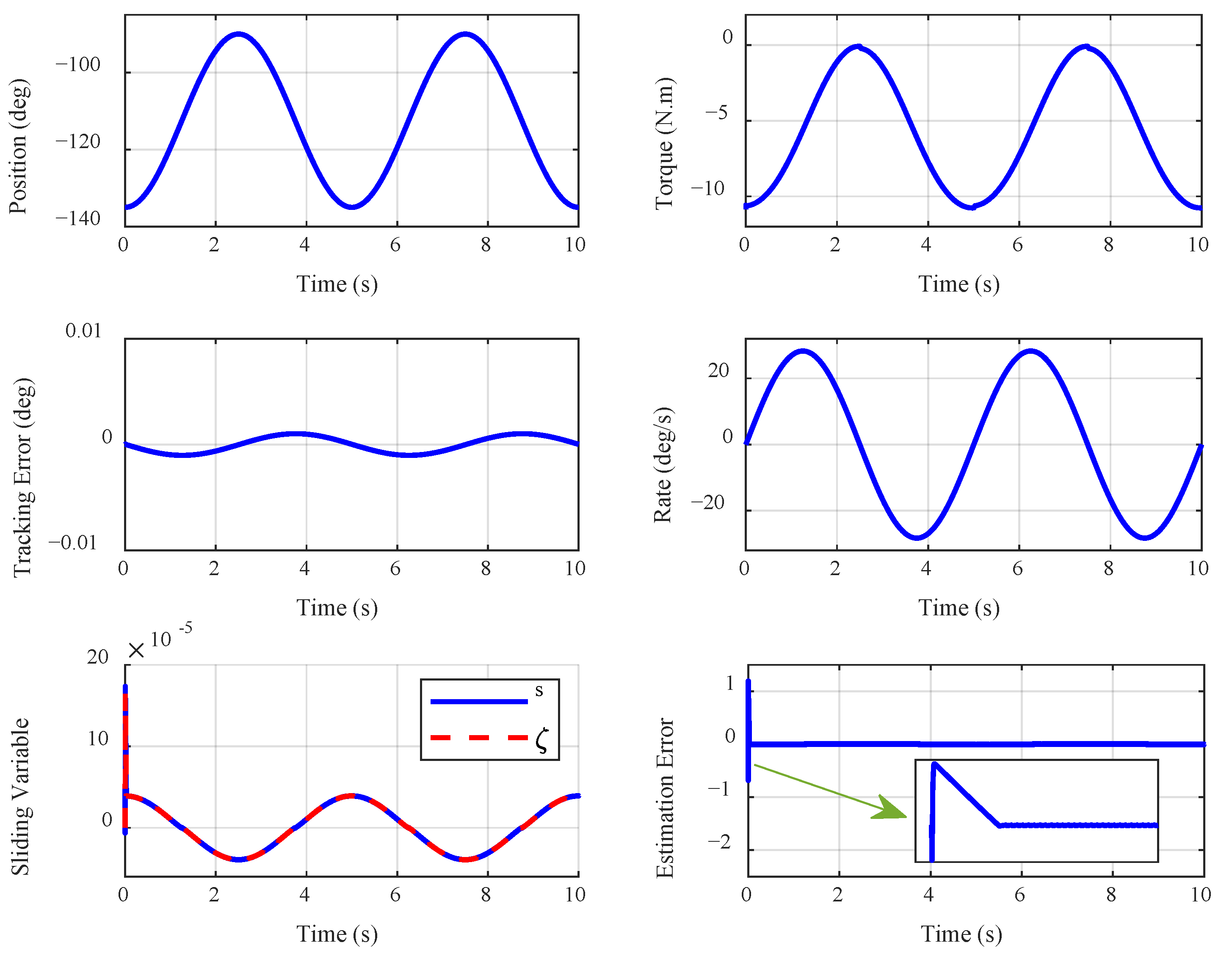
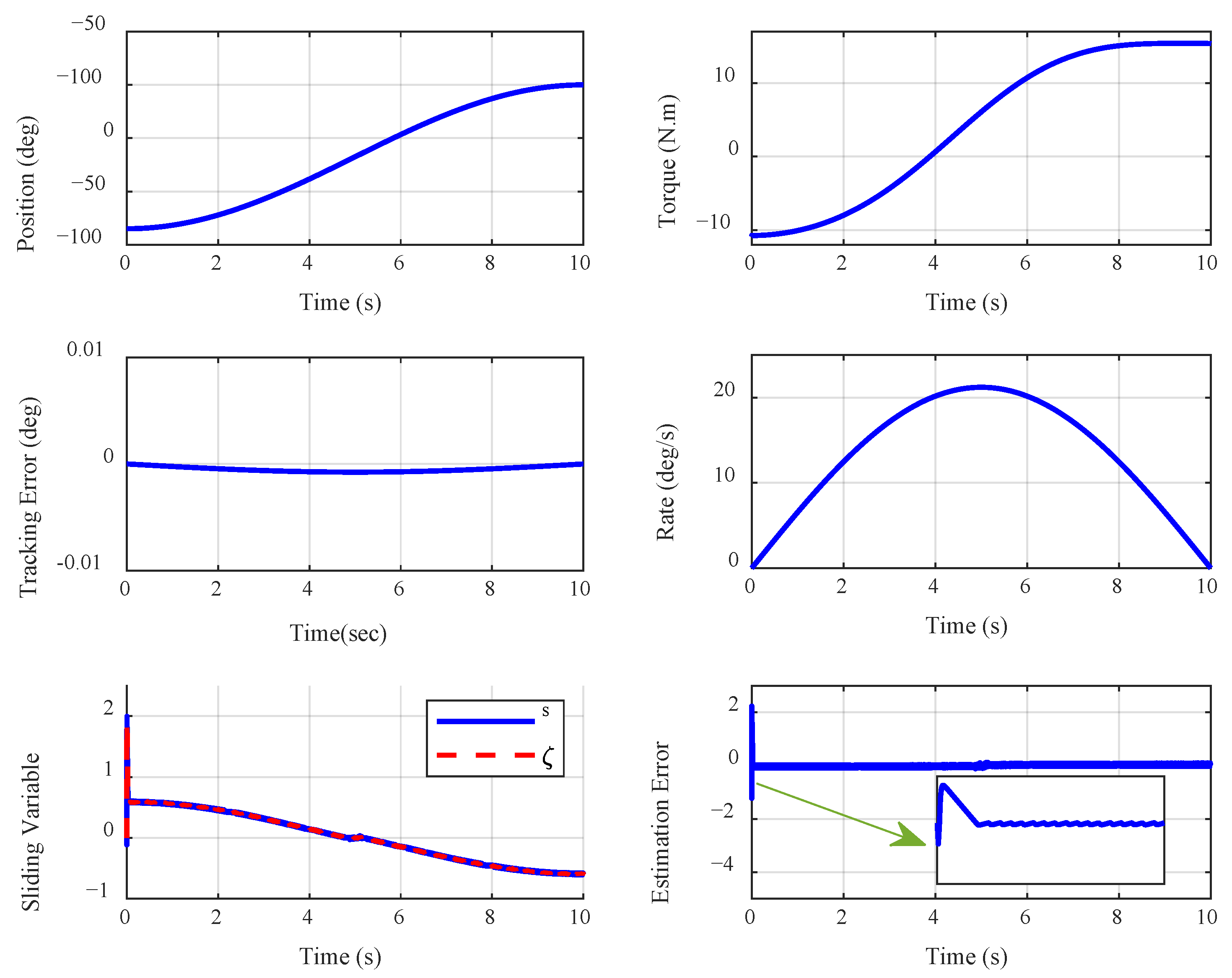
4.1. Examining the Impact of Knee Position Variation

In this section, we scrutinize the proposed control system performance in tracking various desired knee angles. The curves representing these angles are depicted in Figure 7. The first mode examines the transition from total extension to rest. In the second mode, we evaluate the transition from maximal flexion to rest. Finally, in the third mode, the transition from maximal flexion to total extension is assessed.

In the transition from total extension to rest (${\theta }_{d_1}$), the results are illustrated in Figure 8. The desired angle tracking has been achieved with high precision, evidenced by the convergence of both the tracking error and the sliding variable to zero with acceptable accuracy. The controller-generated torque signal exhibits smoothness without any chattering, attributed to the utilization of SOSM theory. Additionally, the sliding variable is estimated with commendable accuracy, and notably, this scenario is devoid of uncertainty or disturbance.

In the state of maximal flexion, transitioning to the rest position (${\theta }_{d_2}$), the results are displayed in Figure 9. The tracking of the desired angle has been executed with comparable precision to the previous case, with both the tracking error and the sliding variable converging to zero accurately. The torque signal generated by the controller remains smooth and devoid of chattering, owing to the application of SOSM theory. Furthermore, the sliding variable is estimated to have high accuracy and velocity. Notably, this scenario is also free from uncertainty and disturbance.

In the state of maximal flexion, transitioning to the rest position (${\theta }_{d_3}$), the results are depicted in Figure 10. The tracking of the desired angle has been performed with good precision, consistent with the two previous cases. Both the tracking error and the sliding variable have converged to zero with acceptable accuracy. The torque signal generated by the controller is smooth and devoid of any chattering, attributable to the application of SOSM theory. Moreover, the sliding variable is estimated with high accuracy and rapidity. Importantly, this scenario does not involve any uncertainty or disturbance.

In Figure 11, the tracking accuracy of these control strategies was evaluated using the ISE (Integral of Squared Error) and ITSE (Integral of Time-weighted Squared Error) indices. The small values indicate high tracking accuracy, with the highest accuracy observed in the scenario of maximal flexion to total extension.

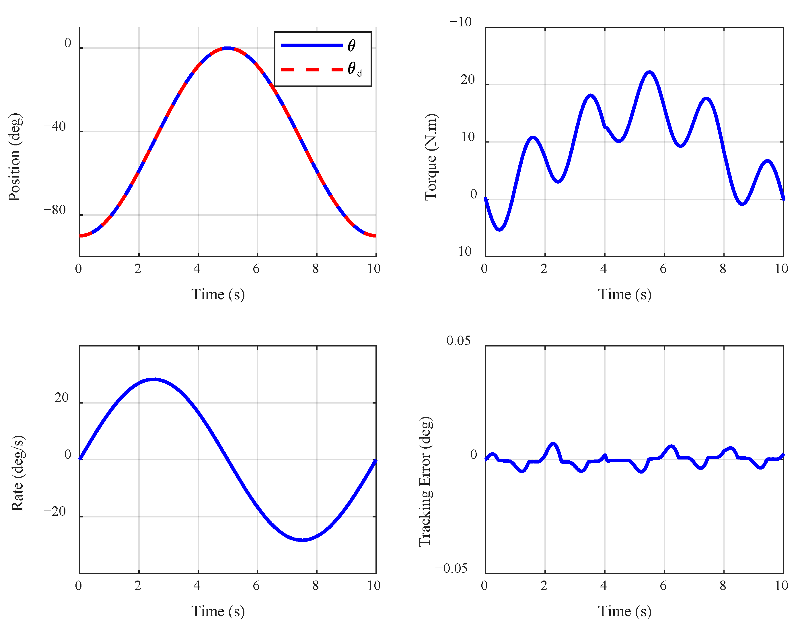
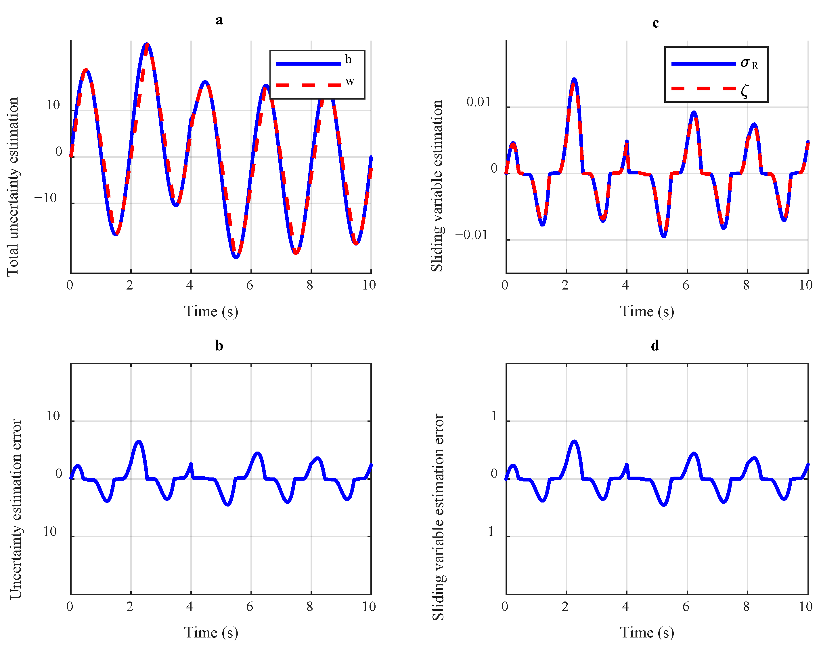
4.2. Analysis of the Impact of Human Torque Variation

In this scenario, we investigate the proposed control system’s robustness against two distinct disturbances: the reaction of the patient’s foot and a 20 percent uncertainty in the model parameters. The curves depicting these disturbances and the overall system uncertainty in this scenario are illustrated in Figure 12.

In the presence of the ${\mathsf{\tau }}_1$ as a human reaction torque disturbance and a 20 percent parametric uncertainty, the results are displayed in Figure 13 and Figure 14. The desired angle is tracked with satisfactory precision despite the disturbance and uncertainty, and the controller generates a smooth signal. Additionally, the sliding variable and the uncertainty of the system are estimated with high accuracy. Armed with this information, the proposed controller successfully tracks the desired output even amidst uncertainty.

In the presence of ${\mathsf{\tau }}_2$ as the human reaction torque and a 20 percent parametric uncertainty, the results are presented in Figure 15 and Figure 16. The desired angle is tracked with satisfactory precision, despite the disturbance and uncertainty which have a slight impact on the precision of tracking. The controller issues a smooth signal. Moreover, the sliding variable and the uncertain component of the system are estimated with high accuracy and speed in this case as well.

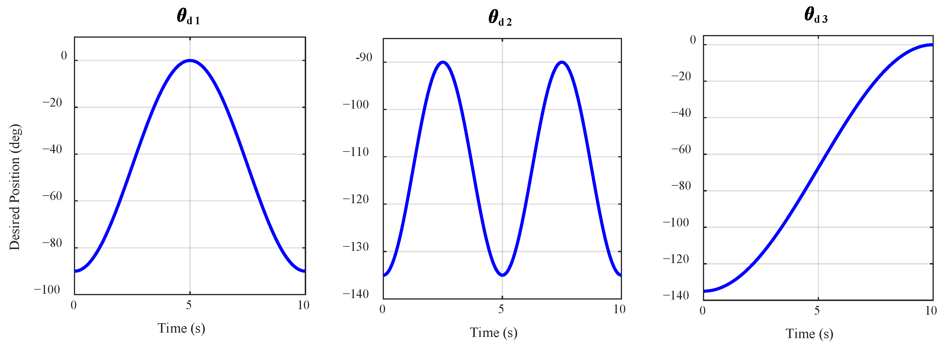
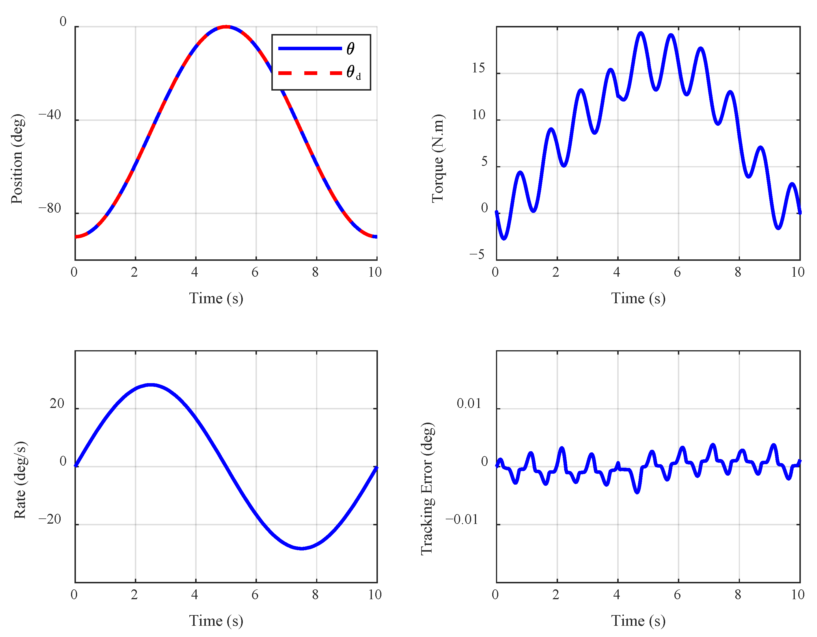
4.3. Investigation of System Behavior for Three Different Subjects

In this scenario, the proposed control system performance is checked across three distinct cases. The details for each individual are provided in

Table 3. System parameter values across three different subjects.

	$\mathit{J}(\mathbf{k}\mathbf{g}·{\mathbf{m}}^2)$	${\mathit{\tau }}_{\mathit{g}}(\mathbf{N}·\mathbf{m})$	$\mathit{A}(\mathbf{N}·\mathbf{m}·\mathbf{s}·\mathbf{r}\mathbf{a}{\mathbf{d}}^{-1})$	$\mathit{B}(\mathbf{N}·\mathbf{m})$
${\mathit{S}}_1$	0.326	15.39	0.354	0.064
${\mathit{S}}_2$	0.359	13.23	0.361	0.085
${\mathit{S}}_3$	0.314	17.59	0.387	0.041

. It can be noted that the proposed control system accounts for the variations in each person’s parameters as a form of parametric uncertainty.

The simulation results for this scenario are shown in Figure 17. The proposed control law, utilizing data solely from the first individual, effectively manages the knee angles for both the second and third individuals. Notably, the controller demonstrates its ability to generate distinct control signals tailored to each individual, achieving comparable control outcomes. This highlights the adaptability of the approach in handling variability among subjects.

Furthermore, the figure reveals that the tracking error and sliding variable consistently converge to an acceptable level. This convergence pattern underscores the robustness of the control design. However, it is worth noting subtle differences in convergence rates and control behavior among individuals, which could be attributed to variations in physiological dynamics. These differences warrant further examination to understand their implications on the control system’s generalizability.

In practical terms, these results suggest that the proposed control law holds promise for personalized yet universal applications, enabling precise management of knee angles across diverse individuals.

5. Conclusions

In this study, we present a pioneering investigation of a knee exoskeleton model, unveiling a cutting-edge finite-time, PID non-singular terminal modified second-order super-twisting SMC scheme. Augmented with an uncertainty estimator, this scheme orchestrates precise regulation of the knee joint angle amidst the system’s inherent nonlinearities, uncertainties, and disturbances. Leveraging estimation insights, our methodology accurately quantifies system uncertainties, thereby facilitating the generation of seamlessly smooth control signals emblematic of second-order SMC behavior. Crucially, our approach ensures robust closed-loop system stability through rigorous Lyapunov analysis, assuming that the upper bound of the uncertainty and its derivative are known, while meticulously calculated convergence time significantly enhances performance predictability. Extensive simulation results affirm the efficacy of our method, particularly in augmenting tracking accuracy and mitigating chattering phenomena. The proposed method demonstrated robustness against parameter uncertainties arising from inaccuracies in robot parameter values and disturbances caused by unwanted patient reactions. It also performed effectively across patients with varying characteristics without requiring control gain adjustments. These findings underscore the pivotal role of our approach in advancing knee exoskeleton control technology and show promise for real-world users and a wide range of operating conditions.

References

1. Yang, X.; Guo, S.; Wang, P.; Wu, Y.; Niu, L.; Liu, D. Design and Optimization Analysis of an Adaptive Knee Exoskeleton. Chin. J. Mech. Eng. 2024, 37, 104. [Google Scholar]
2. Iqbal, J.; Tsagarakis, N.; Fiorilla, A.E.; Caldwell, D. Design requirements of a hand exoskeleton robotic device. In Proceedings of the 14th IASTED International Conference on Robotics and Applications (RA), Cambridge, MA, USA, 2–4 November 2009; pp. 44–51. [Google Scholar]
3. Yan, M.; Gao, G.; Chen, X.; Xing, Y.; Lu, S. Human-Mechanical Biomechanical Analysis of a Novel Knee Exoskeleton Robot for Rehabilitation Training. In Proceedings of the The International Conference on Applied Nonlinear Dynamics, Vibration and Control, Hong Kong, China, 4–6 December 2023; pp. 390–402. [Google Scholar]
4. Wu, Z.; Yang, M.; Xia, Y.; Wang, L. Mechanical structural design and actuation technologies of powered knee exoskeletons: A review. Appl. Sci. 2023, 13, 1064. [Google Scholar] [CrossRef]
5. Iqbal, J.; Tsagarakis, N.G.; Caldwell, D.G. A human hand compatible optimised exoskeleton system. In Proceedings of the 2010 IEEE International Conference on Robotics and Biomimetics, Tianjin, China, 14–18 December 2010; pp. 685–690. [Google Scholar]
6. Preethichandra, D.; Piyathilaka, L.; Sul, J.-H.; Izhar, U.; Samarasinghe, R.; Arachchige, S.D.; de Silva, L.C. Passive and Active Exoskeleton Solutions: Sensors, Actuators, Applications, and Recent Trends. Sensors 2024, 24, 7095. [Google Scholar] [CrossRef] [PubMed]
7. Arefeen, A.; Xiang, Y. Subject specific optimal control of powered knee exoskeleton to assist human lifting tasks under controlled environment. Robotica 2023, 41, 2809–2828. [Google Scholar]
8. Iqbal, J.; Ahmad, O.; Malik, A. HEXOSYS II-towards realization of light mass robotics for the hand. In Proceedings of the 2011 IEEE 14th International Multitopic Conference, Karachi, Pakistan, 22–24 December 2011; pp. 115–119. [Google Scholar]
9. Chen, Z.; Guo, Q.; Li, T.; Yan, Y. Output constrained control of lower limb exoskeleton based on knee motion probabilistic model with finite-time extended state observer. IEEE/ASME Trans. Mechatron. 2023, 28, 2305–2316. [Google Scholar]
10. Yao, Y.; Shao, D.; Tarabini, M.; Moezi, S.A.; Li, K.; Saccomandi, P. Advancements in Sensor Technologies and Control Strategies for Lower-Limb Rehabilitation Exoskeletons: A Comprehensive Review. Micromachines 2024, 15, 489. [Google Scholar] [CrossRef]
11. Zhang, L.; Zhang, X.; Zhu, X.; Wang, R.; Gutierrez-Farewik, E.M. Neuromusculoskeletal model-informed machine learning-based control of a knee exoskeleton with uncertainties quantification. Front. Neurosci. 2023, 17, 1254088. [Google Scholar]
12. Kuber, P.M.; Rashedi, E. Training and Familiarization with Industrial Exoskeletons: A Review of Considerations, Protocols, and Approaches for Effective Implementation. Biomimetics 2024, 9, 520. [Google Scholar] [CrossRef]
13. Barkataki, R.; Kalita, Z.; Kirtania, S. Anthropomorphic design and control of a polycentric knee exoskeleton for improved lower limb assistance. Intell. Serv. Robot. 2024, 17, 555–577. [Google Scholar]
14. Lin, C.-J.; Sie, T.-Y. Design and experimental characterization of artificial neural network controller for a lower limb robotic exoskeleton. Actuators 2023, 12, 55. [Google Scholar] [CrossRef]
15. Masengo, G.; Zhang, X.; Dong, R.; Alhassan, A.B.; Hamza, K.; Mudaheranwa, E. Lower limb exoskeleton robot and its cooperative control: A review, trends, and challenges for future research. Front. Neurorobot. 2023, 16, 913748. [Google Scholar]
16. Ehsani, M.; Oraee, A.; Abdi, B.; Behnamgol, V.; Hakimi, S. Adaptive Dynamic Sliding Mode Algorithm for BDFIG Control. Iran. J. Electr. Electron. Eng. 2023, 19, 2405. [Google Scholar]
17. Liu, J.; Zhang, Y.; Wang, J.; Chen, W. Adaptive sliding mode control for a lower-limb exoskeleton rehabilitation robot. In Proceedings of the 2018 13th IEEE Conference on Industrial Electronics and Applications (ICIEA), Wuhan, China, 31 May–2 June 2018; pp. 1481–1486. [Google Scholar]
18. Mefoued, S. A second order sliding mode control and a neural network to drive a knee joint actuated orthosis. Neurocomputing 2015, 155, 71–79. [Google Scholar]
19. Gol, V.B.; Ghahramani, N. Design of a New Proportional Guidance Algorithm Using Sliding Mode Control. Aerosp. Mech. J. 2014, 10, 77–86. [Google Scholar]
20. Utkin, V.; Poznyak, A.; Orlov, Y.; Polyakov, A. Conventional and high order sliding mode control. J. Frankl. Inst. 2020, 357, 10244–10261. [Google Scholar]
21. Khamar, M.; Edrisi, M. Designing a backstepping sliding mode controller for an assistant human knee exoskeleton based on nonlinear disturbance observer. Mechatronics 2018, 54, 121–132. [Google Scholar]
22. Gogani, N.S.; Behnamgol, V.; Hakimi, S.; Derakhshan, G. Finite time back stepping supper twisting controller design for a quadrotor. Eng. Lett. 2022, 30, 674–680. [Google Scholar]
23. Alouane, S.; Djeghali, N.; Bettayeb, M.; Hamoudi, A. High-order sliding mode-based robust active disturbance rejection control for uncertain fractional-order nonlinear systems. Int. J. Syst. Sci. 2025, 1–21. [Google Scholar] [CrossRef]
24. Ehsani, M.; Oraee, A.; Abdi, B.; Behnamgol, V.; Hakimi, M. Adaptive dynamic sliding mode controller based on extended state observer for brushless doubly fed induction generator. Int. J. Dyn. Control. 2024, 12, 3719–3732. [Google Scholar] [CrossRef]
25. Zhufu, G.; Wang, S.; Wang, X. Finite time disturbance observer based sliding mode control for PMSM with unknown disturbances. Int. J. Robust Nonlinear Control 2024, 34, 7547–7564. [Google Scholar] [CrossRef]
26. Mefoued, S.; Belkhiat, D.E.C. A robust control scheme based on sliding mode observer to drive a knee-exoskeleton. Asian J. Control. 2019, 21, 439–455. [Google Scholar]
27. Behnamgol, V.; Asadi, M.; Mohamed, M.A.A.; Aphale, S.S.; Niri, M.F. Comprehensive review of lithium-ion battery state of charge estimation by sliding mode observers. Energies 2024, 17, 5754. [Google Scholar] [CrossRef]
28. Zhang, J.; Gao, W.; Guo, Q. Extended State Observer-Based Sliding Mode Control Design of Two-DOF Lower Limb Exoskeleton. Actuators 2023, 12, 402. [Google Scholar] [CrossRef]
29. Gao, P.; Zhang, G.; Ouyang, H.; Mei, L. An adaptive super twisting nonlinear fractional order PID sliding mode control of permanent magnet synchronous motor speed regulation system based on extended state observer. IEEE Access 2020, 8, 53498–53510. [Google Scholar] [CrossRef]
30. Yu, X.; Feng, Y.; Man, Z. Terminal sliding mode control–an overview. IEEE Open J. Ind. Electron. Soc. 2020, 2, 36–52. [Google Scholar]
31. Behnamgol, V.; Vali, A.R. Terminal sliding mode control for nonlinear systems with both matched and unmatched uncertainties. Iran. J. Electr. Electron. Eng. 2015, 11, 109–117. [Google Scholar]
32. Mao, Y.; Chen, J. Nonsingular Fast Terminal Sliding Mode Neural Network Decentralized Control of a Quadrotor Unmanned Aerial Vehicle. Complexity 2023, 2023, 3288944. [Google Scholar]
33. Sohani, B.; Rahmani, A.; Mercer, K.; Nelson-Smith, O.; Butcher, C.; Hazell, S.; Ren, Y.; Aliyu, A.; Goher, K. Optimising Knee Replacement Surgery: Development and Assessment of a Parallel Kinematic Machine for Precise Positioning in Knee Arthroplasty. In Proceedings of the Climbing and Walking Robots Conference, Kaiserslautern, Germany, 4–6 September 2024; Springer Nature: Cham, Switzerland, 2024. [Google Scholar]
34. Mohammed, S.; Huo, W.; Huang, J.; Rifaï, H.; Amirat, Y. Nonlinear disturbance observer based sliding mode control of a human-driven knee joint orthosis. Robot. Auton. Syst. 2016, 75, 41–49. [Google Scholar]
35. Mahdi, S.M.; Yousif, N.Q.; Oglah, A.A.; Sadiq, M.E.; Humaidi, A.J.; Azar, A.T. Adaptive synergetic motion control for wearable knee-assistive system: A rehabilitation of disabled patients. Actuators 2022, 11, 176. [Google Scholar] [CrossRef]
36. Rifaï, H.; Mohammed, S.; Hassani, W.; Amirat, Y. Nested saturation based control of an actuated knee joint orthosis. Mechatronics 2013, 23, 1141–1149. [Google Scholar]
37. Khan, A.H.; Li, S. Sliding mode control with PID sliding surface for active vibration damping of pneumatically actuated soft robots. IEEE Access 2020, 8, 88793–88800. [Google Scholar]
38. Shao, X.; Sun, G.; Xue, C.; Li, X. Nonsingular terminal sliding mode control for free-floating space manipulator with disturbance. Acta Astronaut. 2021, 181, 396–404. [Google Scholar]
39. Plestan, F.; Shtessel, Y.; Bregeault, V.; Poznyak, A. New methodologies for adaptive sliding mode control. Int. J. Control 2010, 83, 1907–1919. [Google Scholar]
40. Shtessel, Y.B.; Shkolnikov, I.A.; Levant, A. Smooth second-order sliding modes: Missile guidance application. Automatica 2007, 43, 1470–1476. [Google Scholar]
41. Behnamgol, V.; Vali, A.R.; Mohammadi, A. A new adaptive finite time nonlinear guidance law to intercept maneuvering targets. Aerosp. Sci. Technol. 2017, 68, 416–421. [Google Scholar] [CrossRef]
42. Yang, J.; Yu, X.; Zhang, L.; Li, S. A Lyapunov-based approach for recursive continuous higher order nonsingular terminal sliding-mode control. IEEE Trans. Autom. Control 2020, 66, 4424–4431. [Google Scholar]
Figure 1. Mechanical structure of an orthosis [18].
Electronics 14 01455 g001
Figure 2. Fixed and Shank Coordinate Frames [35].
Electronics 14 01455 g002
Figure 3. (a,b): Variations of θ and its rate in the absence of uncertainties; (c,d): variations of θ and its rate in the presence of τ h as human reflection and 20% of uncertainty in all parameters.
Electronics 14 01455 g003
Figure 4. The structure of σ R in the recursive PID non-singular TSM variable.
Electronics 14 01455 g004
Figure 5. Proposed switching control law structure.
Electronics 14 01455 g005
Figure 6. The closed-loop system block diagram.
Electronics 14 01455 g006
Figure 7. The closed-loop system block diagram. Three desired trajectories of knee angle: ( θ d 1 ) total extension to rest, demonstrating the system’s ability to manage stabilized movements. ( θ d 2 ) maximal flexion to rest, showcasing control across a reduced range of motion. ( θ d 3 ) maximal flexion to total extension, highlighting control across the full range of motion.
Electronics 14 01455 g007
Figure 8. System characteristics with θ d 1 representing the desired position, assuming no uncertainty or human torque is present.
Electronics 14 01455 g008
Figure 9. System characteristics with θ d 2 representing the desired position, assuming no uncertainty or human torque is present.
Electronics 14 01455 g009
Figure 10. System characteristics with θ d 3 representing the desired position, assuming no uncertainty or human torque is present.
Electronics 14 01455 g010
Figure 11. Comparison of ISE and ITSE in three knee position scenarios.
Electronics 14 01455 g011
Figure 12. ( τ 1 ) and ( τ 2 ) represent the human reaction torque, whereas ( h 1 ) and ( h 2 ) signify the total uncertainty, which includes 20% parametric uncertainty and external disturbances.
Electronics 14 01455 g012
Figure 13. System characteristics in the presence of τ h 1 representing human torque and 20% parametric uncertainty.
Electronics 14 01455 g013
Figure 14. (a) Curves of w and h; (b) estimation error of h; (c) curves of σ and ξ ; (d) estimation error of sliding variable, in the presence of τ h 1 representing human reflex and 20% parametric uncertainty.
Electronics 14 01455 g014
Figure 15. System characteristics in the presence of τ h 2 representing human torque and 20% parametric uncertainty.
Electronics 14 01455 g015
Figure 16. (a) Curves of w and h; (b) estimation error of h; (c) curves of σ and ξ ; (d) estimation error of sliding variable, in the presence of τ h 2 representing human reflex and 20% parametric uncertainty.
Electronics 14 01455 g016
Figure 17. Performance of the proposed controller for controlling three different subjects.
Electronics 14 01455 g017