Abstract
This article presents an improved control strategy based on the traditional sliding-mode controller (SMC), integrated with a generalized higher-order disturbance observer (DOB), to enhance the speed regulation of permanent magnet synchronous motors (PMSMs) during operation. The proposed method is mitigated and employed to smooth system disturbances by utilizing the disturbance observer (DOB) in conjunction with a low-pass filter (LPF). The low-pass filter is employed to smooth the q-axis current component and reduce speed oscillations. Initially, the paper builds upon the conventional control law and introduces a more optimized approach. The stability of the control strategy is then analyzed using Lyapunov stability theory. Different sliding surfaces are compared to develop the proposed SMC. Finally, the novel control method is introduced by integrating the DOB with the LPF. This approach results in improved speed stability and enhanced adaptability compared to traditional SMC techniques. Simulation and experimental results demonstrate that the proposed control algorithm outperforms traditional methods, particularly in terms of the dynamic response and disturbance rejection.
1. Introduction
Currently, with the development of power electronics [1] and the wide usage of materials with high magnetic properties [2], as well as putting forward a timetable for electric vehicles to replace fossil-fuel-based vehicles [3], research into electric motors is of increasing interest and becoming more popular. The application of PMSM motors is increasing rapidly in the industrial sector, as well as in rail transit applications [4] and electric vehicles [3], due to their efficiency advantages and high power density. Vector control [5] is one of the most classical control strategies for PMSM motors. The speed controller in a vector control system that controls speed in an alternating current (AC) system with a PMSM usually uses a traditional control [6]. This method’s algorithm features simplicity, high reliability, and convenient parameter setting. Nevertheless, since the PMSM constitutes a strongly coupled, non-linear control system, external disturbances or the motor’s internal variable parameters constantly impact the control system. The above facts show that it will be quite difficult to achieve high-performance PMSM control by using some traditional control methods, such as Linear Quadratic Regulator (LQR) control [7] or PID control systems.
There are two primary types of PMSM control methods: traditional linear methods like PID [6], LQR [7], and Exact Model Matching (EMM) control [8]. While PI controllers are commonly used for position and speed control, they have limitations, such as poor robustness to parameter variations and difficulties in tuning. LQR offers simplicity in its design but lacks a precise method for determining optimal Q and R matrices. EMM aims to meet time and frequency domain specifications but may not guarantee physical hardware implementation.
The second method involves nonlinear control theory, particularly for high-speed PMSM applications. Integrated speed and current controllers have been employed to manage the nonlinear coupling between the speed and current. Various advanced nonlinear control strategies have emerged recently to enhance speed regulation in PMSM motors across different applications. These include neural network control [9], backstepping control [10], automatic disturbance rejection control [11], fuzzy logic control (FLC) [12], predictive control [13], AI-based control [14], SMC [15], variable structure control [16], predictive current control (PCC) [17], disturbance observer (DOB) [18], and extended state observer (ESO) [19]. Among these, SMC stands out for its robustness against disturbances and reduced reliance on precise system parameter knowledge. However, the sliding-mode method has its drawbacks. In practical applications, the switching control laws often experience time delays. These delays give rise to high-frequency dynamics, a phenomenon commonly referred to as chattering. L. Feng et al. [20] improved the coefficient of the variable speed reaching law from a constant to a fraction that changes with the state variable x and used a new sliding-mode surface for the improved nonsingular fast terminal sliding-mode controller. However, the speed of the reaching law has not yet reached the desired speed, and the coefficient of the variable index reaching law has not changed, so chattering is still not limited compared to the traditional exponential reaching law. T.H. Nguyen et al. [21] also changed the reaching law; however, the reaching law only has the variable speed reaching law part and ignores the variable index reaching law part, so chattering greatly affects the results.
To solve the problems from the above studies, this article proposes a new sliding surface control law for an improved SMC controller. The proposed approach can mitigate chattering and shorten the time required for the system state to reach the sliding-mode surface. By enhancing the SMC_DOB, it takes into account and overcomes parameter uncertainties and load disturbances. This improvement enables the new sliding-mode control to retain its robustness and reduces the overshoot during a reference speed jump. The main contributions of this paper are as follows:
- A novel sliding-mode control strategy is put forward, which integrates an improved reaching law and a new-type sliding-mode surface. This unique sliding-mode surface has the ability to adapt to changes in both the sliding surface itself and the system states. Through this adaptation, the control strategy intends to minimize chattering and shorten the reaching time.
- To improve the disturbance rejection and robustness of the new sliding-mode control, especially when a reference speed jump occurs, an improvement to the DOB mitigates the impact of disturbances and reduces system overshoot.
- Additionally, the DOB and LPF filter work together to enhance the system’s characteristics and make the transient characteristics smoother than before.
The subsequent sections of this paper are structured as follows: the mathematical models of the PMSM and the new sliding-mode control are designed and analyzed in Section 2. The LPF filter gets integrated into the DOB introduced and analyzed in Section 3. Simulation and experimental results are presented in Section 4. The paper is then concluded in Section 5.
2. Novel Slide Mode Controller Design
2.1. The Mathematical Model of PMSM
In the synchronous rotating reference frame [22], the d-q axis current and moment equations for the stator of the PMSM motor can be formulated as follows:
Here, id and iq represent the stator currents along the d and q axes, respectively; ud and uq signify the stator voltages in the d–q frame; Rs is the stator resistance; ωe denotes the electrical angular speed; ωm represents the mechanical angular speed. Ld, Lq are the inductances along the d axis and q axis, respectively. Moreover, ψf is the permanent magnet (PM) flux linkage. TL represents the load torque, and Te is the electromagnetic torque; p is the number of pole-pairs of the electric machine. Additionally, J and Ba are the moment of inertia and the viscous coefficient of the load, respectively.
In the study, the authors used a surface-mounted PMSM motor, so the d-axis and q-axis inductances in the dq coordinate system are equal: Ld = Lq = L. Thus, in Equation (4), the reluctance moment component does not exist. Then, the motor’s electromagnetic torque is proportional to the transaxial current iq.
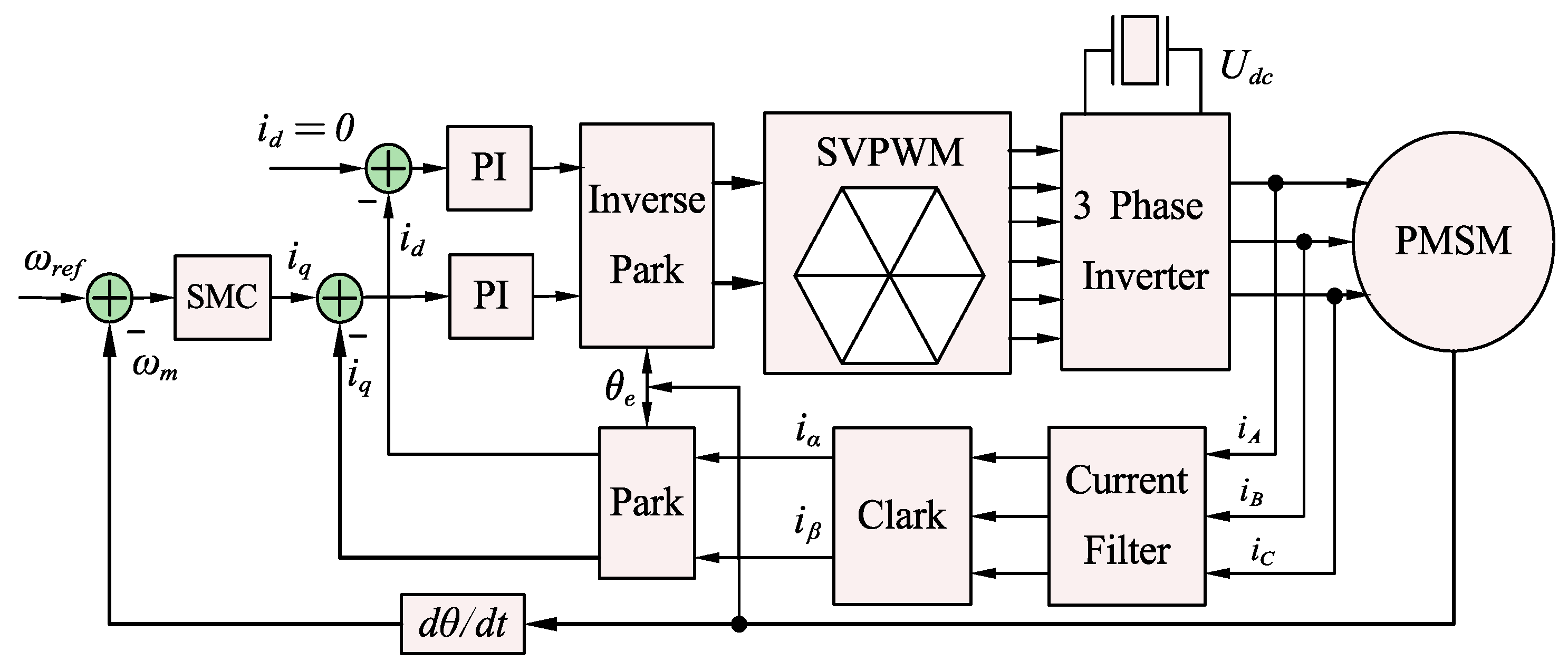
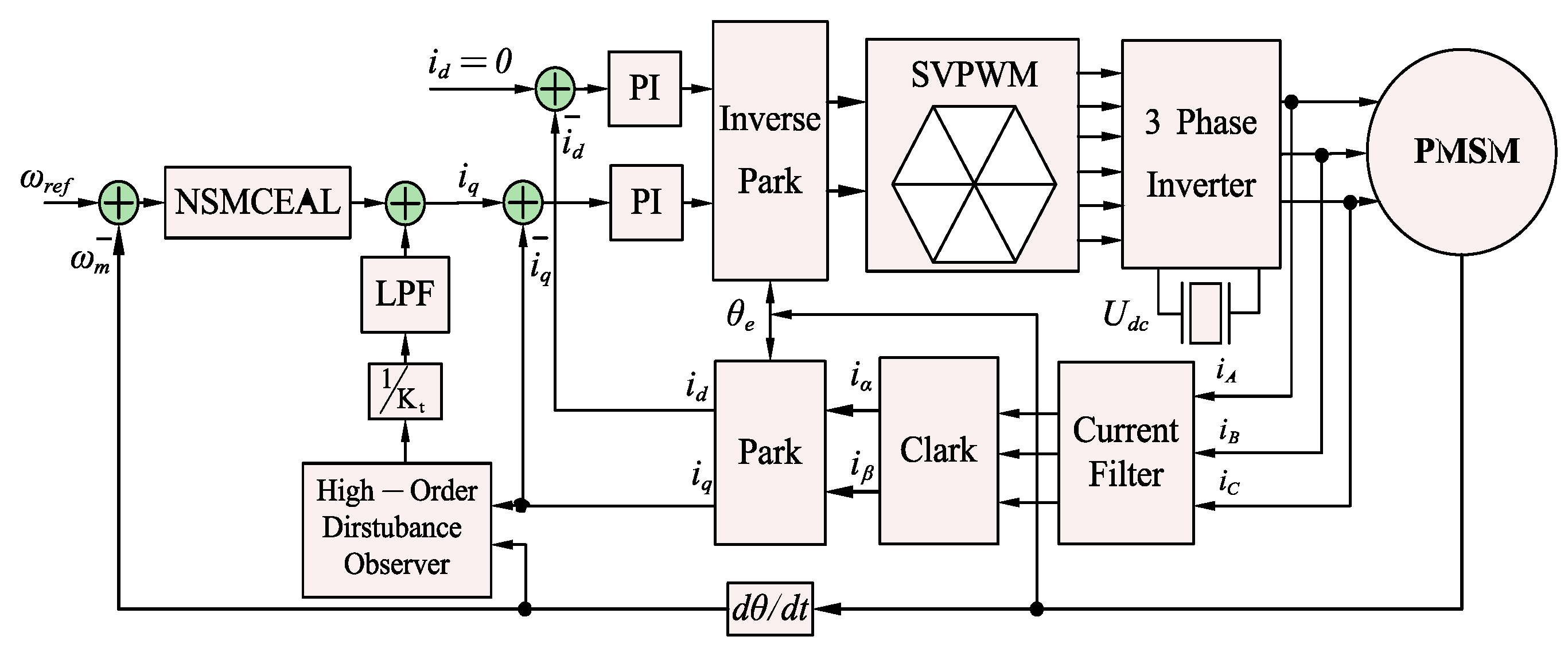
Figure 1 illustrates the control structure of a PMSM system using the FOC method, which includes two current controllers and a speed controller. The current control loop employs a conventional PI algorithm, where the d-axis reference current is set to zero, and the q-axis reference current is determined by the output signal of the speed loop. This study focuses on improving the speed controller.
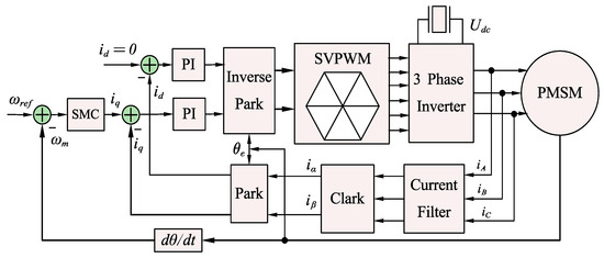
Figure 1.
Diagram illustrating SMC and VSI-FOC configuration in PMSM drive system.
The main characteristics of SMC are determined by the control law structure and the presence of a discontinuous control system on the switching surface. In the traditional SMC, the state trajectory is permitted to get close to a pre-established sliding-mode surface and then converge along this surface in the direction of the state origin. Nevertheless, the stability conditions are unable to illustrate the manner in which the system approaches the SMC regime.
Conversely, selecting the right law method and combining it with an optimal algorithm can guarantee the system’s motion phase quality. Selecting an appropriate reaching law can endow the system with a higher approaching velocity, thereby accelerating the system’s dynamic response when the state vector is distant from the sliding-mode surface. Once the system arrives at the sliding-mode surface, the approaching velocity is decreased to zero to ensure that the state vector remains in a steady state on this surface. Subsequently, the following is an example of a typical system:
The derivative of the sliding-mode surface function, which is based on the conventional exponential approach law (CEAL), is expressed as follows:
In this context, the term εsgn(s) represents the isokinetic reach component, while qs stands for the index reach component. The variable s denotes a sliding-mode surface function.
Regarding the CEAL, reaching the sliding-mode surface in a limited amount of time is unfeasible. Therefore, the isokinetic reach term εsgn(s) is added to ensure that when s is close to 0, the reaching velocity is ε instead of 0.
However, while the addition of the isokinetic reach term resolves the accessibility issue, the rate at which the exponential reaching law arrives at the sliding-mode surface is set by the parameter q’s design value. This gives rise to a conundrum: enhancing the approach speed runs counter to the aim of minimizing sliding chattering. To determine the reaching time of the sliding-mode surface, integrate Equation (6) from 0 to t with parameter s:
When 0 < s < t, the expression εsgn(s) is equal to ε. Once the system reaches the sliding-mode surface, s(t) = 0. The reaching time is expressed as follows:
According to Equation (8), to achieve swifter reaching performance, the value of q needs to be raised. However, a large q results in an overly high speed upon reaching the sliding surface, thereby augmenting the chattering level. Consequently, if the coefficient of the index term can be made variable and its value is correlated with the distance between the system state point and the sliding-mode surface, the conflict stemming from the selection of the q value can be resolved. This concept paves the way for the proposal of the new law in the subsequent paragraphs.
2.2. Proposed NSMCEAL Design
Drawing on the conventional exponential reaching law, the novel SMC exponential approach law (NSMCEAL) can adapt to the changes in the sliding-mode surface and system state. The formulation of this reaching law is as follows:
Regarding the reaching law, x indicates the system state.
In the system, the state approaches the sliding-mode surface in accordance with two distinct laws: the variable speed reaching law and the variable-index reaching law. F(x,t) is an additional function in the sign coefficient of the traditional variable speed reaching law. For the coefficient of the variable index reaching law, the function G(s) is added to help improve the sliding-mode.
The first, . The term is nonlinear because of the exponential function , which is the function of the magnitude of the sliding-mode surface function s. As |s| increases, decreases. Since is in the numerator of F(x,t), when |s| increases, increases from a value close to 1 towards as . Therefore |s|, to simplify (when |x|), and |s|, the function to .
For can be split into cases based on the sgn of s. When s > 0, , and when s < 0, . This shows that the influence of the qG(s) term on changes depending on the sgn and magnitude of the sliding-mode surface function s. This phenomenon indicates that as the system state gets closer to the sliding-mode surface, the coefficients of the reaching law gradually decrease, which helps to reduce chattering.
By analyzing and comparing the performance of each sliding rule, it is possible to show the advantages and disadvantages of NSMCEAL compared to other sliding rules.
2.3. Performance Analysis of NSMCEAL
In order to make a comparison between the conventional sliding-mode laws and NSMCEAL, the controlled system is delineated as follows:
where f(x,t) is a function that depends on the position instructions; u(t) denotes the control input, and d(t) stands for the external disturbance.
The traditional sliding-mode surface function is as follows:
where c must satisfy the Hurwitz condition, c > 0.
The tracking error, along with the corresponding derivative value, is given by the following:
where xd is the ideal position signal.
For the derivative of Equation (12), it can be obtained that
Utilizing the NSMCEAL and referring to Equations (9) and (13), the enhanced sliding-mode control rate can be expressed as follows:
In addition to sliding-mode controllers based on the CEAL law, where the designed function aims to ensure the quality of the normal motion phase, this study also compares it with the NSMC [20] and ASMC [21].
Utilizing MATLAB’s functionality, a simulation is run to compare the performance of CEAL, NSMC, ASMC and NSMCEAL. The details of the simulation parameters that have been set are presented below: , , b = 133, c = 15, ε = 10, q = 20, α = 0.5, λ = 1 and β = 0.3. The ideal position signal of the system, denoted as xd, is assigned the value of sin(t). Meanwhile, the initial state of the controlled object x(0) is configured as [x1, x2] = [–2, –2].
As depicted in Figure 2, there is a performance comparison chart that illustrates the differences among the CEAL, NSMC, ASMC, and the newly proposed NSMCEAL. The NSMCEAL demonstrates clear superiority over other control laws in tracking a given signal, minimizing position tracking errors, enhancing the convergence speed of position-related differentials, and suppressing noise. Consequently, compared to other approaches, the NSMCEAL proposed in this paper offers the benefits of a faster reaching speed and a more stable controller output.
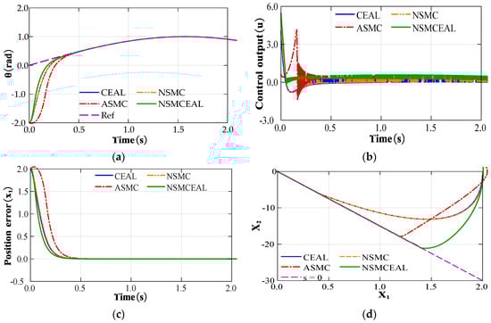
Figure 2.
Performance comparison of CEAL, NSMC, ASMC, and proposed NSMCEAL: (a) tracking performace; (b) control output; (c) position error convergence; (d) phase trajectory.
The proposed NSMCEAL law differs from the CEAL, NSMC, and ASMC laws. Instead of being a fixed constant, the constant speed parameter can change depending on how far away the system state is from the sliding surface. In reaching mode, when the system state is significantly distant from the sliding surface, both the exponential term and the constant speed term operate simultaneously. This causes the system’s reaching speed to increase, enabling the system state to reach the sliding surface within a shorter period of time. During the sliding mode, as the system state gets closer to the sliding mode surface, i.e., s→0, the sliding mode ignores the exponential term qG(s) and applies the constant velocity term. At this time, in the new reaching law ( →), the constant speed term is simplified to ε. When compared with the other laws, the system experiences a smaller decay, quantified by the value ε while on the sliding mode surface. This smaller decay effectively mitigates chattering, leading to a more stable and smoother operation of the system.
2.4. Analysis and Selection of a Novel Sliding-Mode Surface
Using the rotor magnetic field orientation control method with id = 0 can improve control efficiency for PMSM motors with PM mounted on the rotor surface. Given the current conditions, Equations (2) and (3) may be converted into the mathematical model presented below:
Ascertain the state variables associated with the PMSM system:
where ωref denotes the motor’s reference speed, and it is generally maintained as a constant quantity. According to Equations (15)–(17) and (28) it can be seen that
Set , and Equations (19) and (20) become the following:
Regarding sliding surfaces, in addition to conventional sliding-mode surfaces, two other sliding-mode surfaces are currently used: integral sliding-mode surfaces and differential integral sliding-mode surfaces.
The conventional sliding-mode surface (CSMS) function is as follows:
And a differential integral sliding-mode surface (DISMS) [20] is presented as follows:
where C1, C2, C3 > 0 is the parameter to be known.
Differentiating Equation (23), it can be obtained that:
From Equations (19) and (21), then
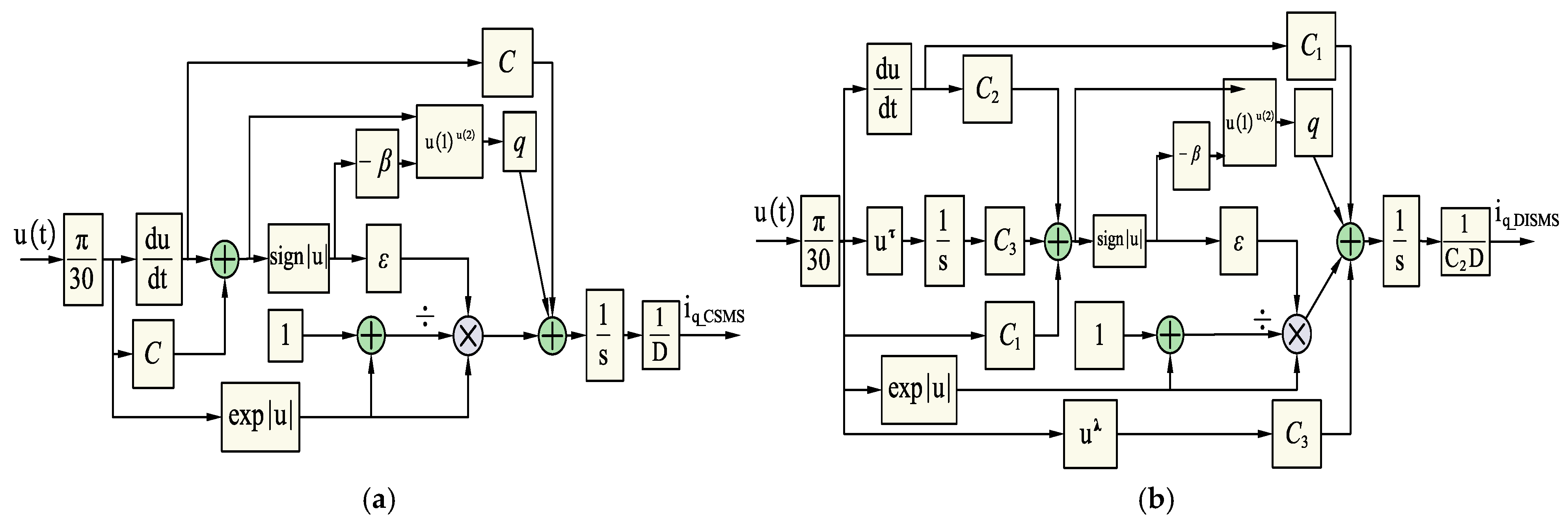
In order to design a sliding-mode controller that guarantees superior dynamic characteristics and tracking capability, the DISMS is employed. By leveraging the novel sliding-mode surface presented in Equation (23), the q-axis current can be expressed as follows:
With the CSMS in Equation (22) sliding surface, the q-axis currents can be described as follows:
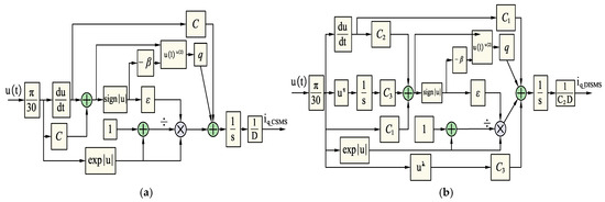
Figure 3.
The model simulates the SMC sliding controller according to sliding surfaces and NSMCEAL laws: (a) CSMS; (b) DISMS.
2.5. Stability Proof
It is possible to create the Lyapunov function as follows:
Combining Equations (9) and (28), the derivation of Equation (28) can be presented:
According to the Lyapunov stability theorem, it can be concluded that the sliding-mode controller designed in this work is progressively stable.
To ensure that the three-phase PMSM drive system has better dynamic quality, the NSMCEAL law with the DISMS surface method is used here, and the expression of the controller can be obtained as follows Equation (26). As can be observed from Equation (26), due to the presence of an integral term within the controller, it offers two significant advantages. Firstly, it has the ability to mitigate the oscillation phenomenon. Secondly, it is capable of eradicating the steady-state error of the system, thereby enhancing the overall quality of the system’s control performance.
3. LPF Filter Gets Integrated into the High-Order Disturbance Observer
Equation (3) expands into the following:
Consider x = ωm, u = Te, K = 1/J, and z = TL (which is a function of motor losses). The system of state equations is as follows:
where A = Ba/J; B = K; C = 1; D = −K; the following formula determines the k-level disturbance observer [23]:
where x is the internal variable of the function, is the estimated value of z, gk represents the kth derivative of the function, and L1, L2, L3,…, Lk+1 are the coefficients of the disturbance observer.
Assuming that the entire noise is a continuous function and the higher-order derivative of the function is bounded above, then we have the following system of disturbance observation matrix equations:
where: , .
The proposed general disturbance observer, of which the function is to estimate the total noise along with its higher-order derivatives, can be constructed as described below:
where the coefficient represents optimal gain of the observer. In the context, W0 is determined by solving the following equation:
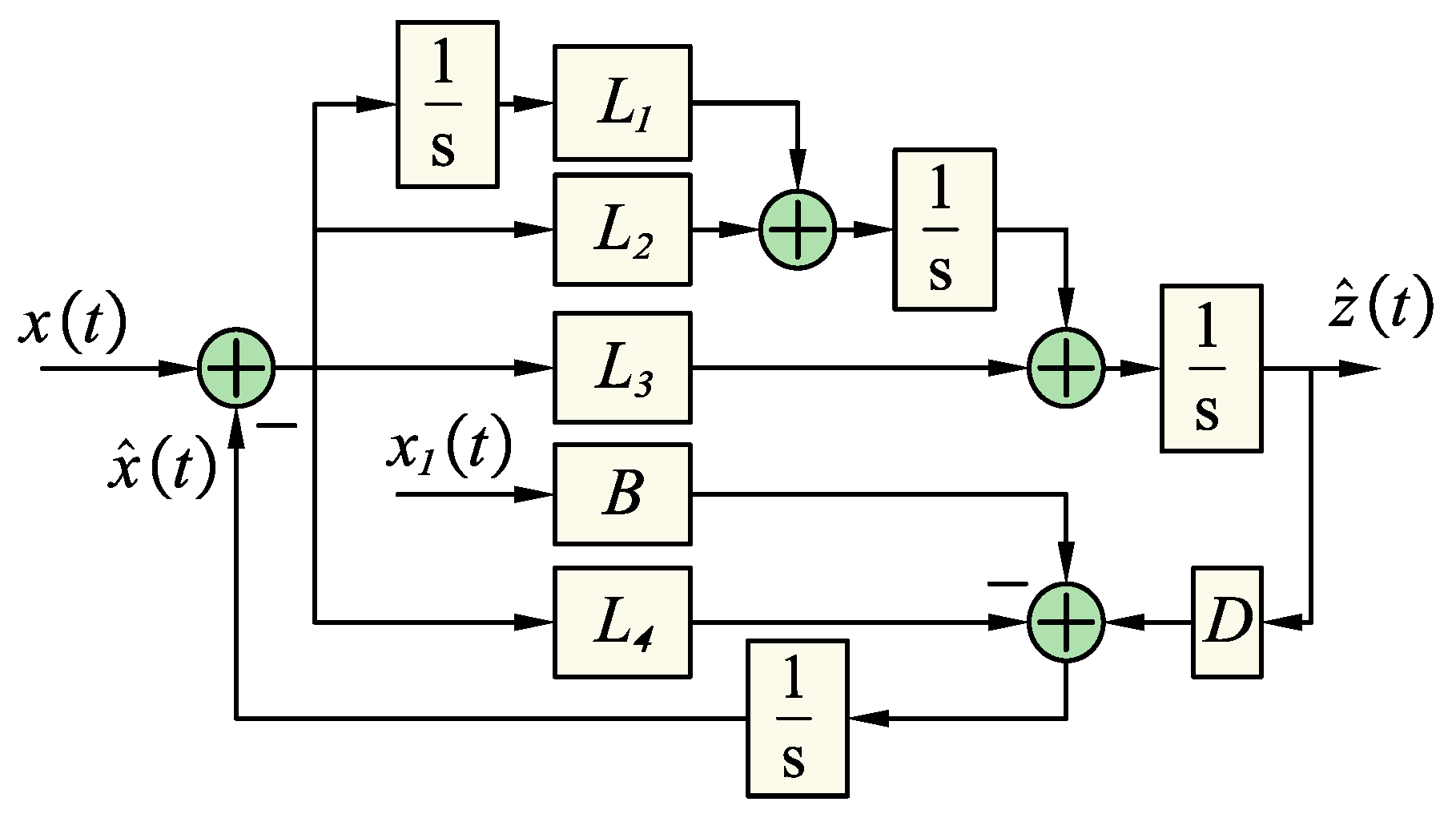
where Q0 and R0 are the weight matrix and scalar coefficients, respectively. When noise occurs, the component of the matrix Q0 will be small, R0 will be large, and vice versa. In the paper, the author will use experience to determine the values L1 to L4 with the observation set used as level 2, with the model built as shown in Figure 4.

Figure 4.
The block diagram of the second-order DOB with k = 2.
The transfer function of the LPF filter is established as described below:
where ωc is the cutoff frequency of the LPF filter. The LPF cutoff frequencies of the methods need to be set to very low values to achieve better detection efficiency, which will slow down the response speed.
Transfer function (36) represents the transfer function of a second-order Butterworth low-pass filter. The Butterworth filter is engineered to exhibit a maximally flat magnitude response within the passband. This characteristic ensures that the signal components falling within the passband undergo minimal distortion. Moreover, this filter is characterized by a simple architecture and relatively low phase delay in the passband. As a result, it can maintain a reasonable response speed while effectively performing noise-filtering operations.
Then, the amplitude of the frequency of the LPF filter will be as follows:
To reduce the magnitude of the fundamental current to 1/10 the harmonic current, should be bigger than 10.
The quadrature current iq of the motor is represented by the output of the SMC sliding-mode controller using the proposed NSMCEAL from Equation (26). To counteract the impact of the total noise, it has been suggested to include an LPF in the observer’s output as shown in Figure 5. As a result, the output quadrature current iq is calculated as follows:
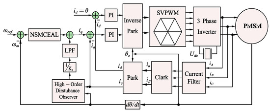
Figure 5.
Block diagram of sliding-mode control model with high-order disturbance observer and low-pass filter for PMSM.
4. Simulation Analysis
4.1. Set Up a Simulation Model
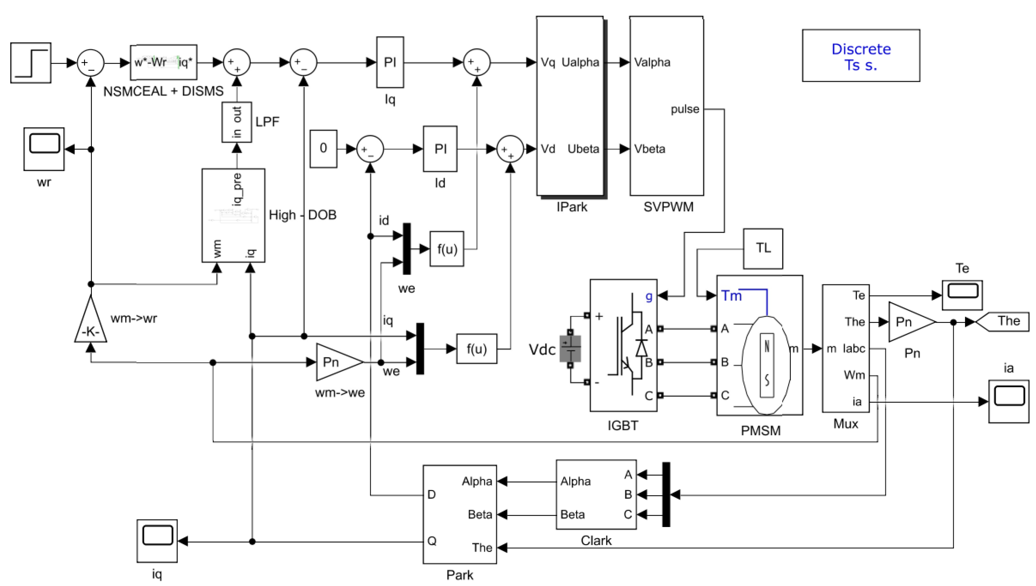
The simulation model of the sliding-mode control algorithm, the high-order disturbance observer, the low-pass filter algorithm, and the PMSM motor are built in MATLAB2019/Simulink as shown in Figure 6. Among them, the motor parameters in the simulation are set as follows in the Table 1.
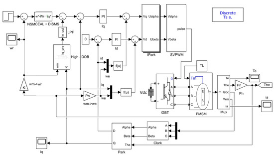
Figure 6.
Sliding-mode control model combined with high-order disturbance observer and low-pass filter for PMSM in MATLAB2019/Simulink.

Table 1.
PMSM motor system parameters.
The DOB observer estimates the disturbance values using the following equations:
The observer gain matrix value L is calculated using Matlab, and it was calculated as follows:
4.2. Simulation Results
4.2.1. Performance Analysis of Traditional Sliding-Mode Surface
This section presents a comparison of the PMSM’s dynamic performance with a constant torque reference of 10 Nm; the speed varies from 800 rpm to 1000 rpm. The control methods employed include CEAL, NSMC [20], ASMC [21], and NSMCEAL, all of which are based on the CSMS, as defined in Equation (24), along with PI control. The sliding-mode laws and parameters of the CSMS are detailed in Table 2.
Table 2.
The gains of the SMC controller and the disturbance observers for the simulation.
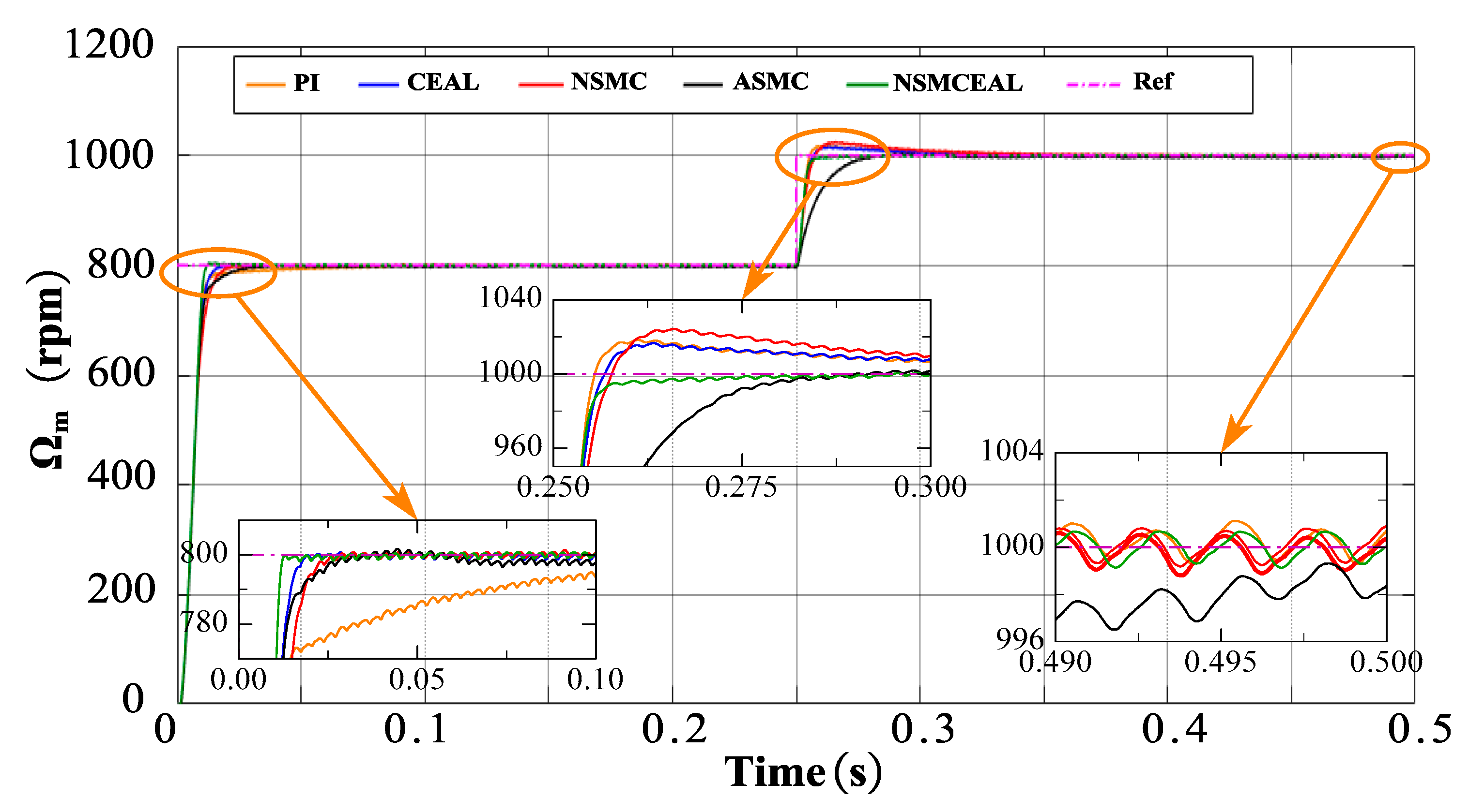
In the speed variation model (Figure 7), it is observed that during startup, the PI controller exhibits a slower convergence time compared to other sliding-mode control methods based on the CSMS. While all methods demonstrate comparable overshoot levels, the proposed NSMCEAL method achieves faster convergence. When the speed is increased from 800 rpm to 1000 rpm, the PI, CEAL, and NSMC methods show significant overshoot, whereas the remaining methods, particularly NSMCEAL, deliver superior performance with minimal overshoot and better stability.
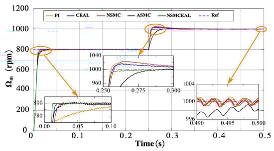
Figure 7.
Simulation results of the CSMS with CEAL, NSMC, ASMC, NSMCEAL, and PI: Ωm = 800 rpm to 1000 rpm and TL = 10 Nm.
To quantitatively validate the performance of the proposed method, several indices are employed, including the root mean square (RMS) [24], overshoot, and speed drop, where Ns represents the number of samples:
To conduct a thorough comparison of controller performance, a comprehensive evaluation method with a maximum score of 5 is employed. Leveraging the simulation outcomes, Table 3 and Figure 8 display the comprehensive evaluation schemes for speed controllers based on the CSMS and PI controllers.
Table 3.
Comparison of performance indices of controllers based on the CSMS.
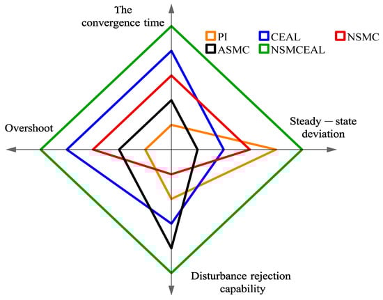
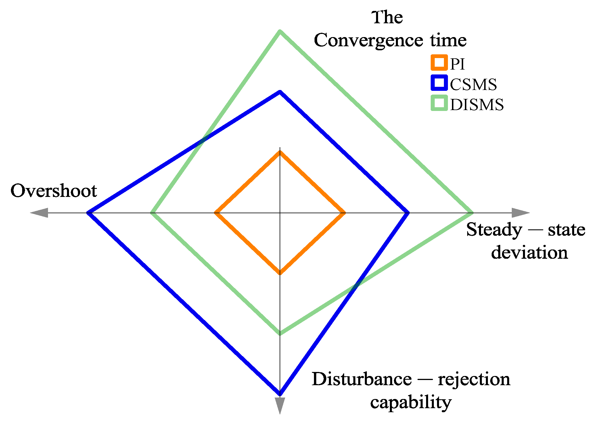
Figure 8.
Radar chart comparing the evaluation of CEAL, NSMC, and NSMCEAL laws based on the CSMS and PI controller.
Figure 8 shows that the controller with the best performance in terms of the convergence speed, steady-state deviation, overshoot, and disturbance rejection capability is the combination of the NSMCEAL law and the CSMS, which demonstrates superior overall performance (indicated by the green line) in the radar chart. The CEAL law and NSMC law with the CSMS surface ranks second.
4.2.2. Evaluating and Comparing the Dynamic Performance of Sliding Surfaces
This section compares the dynamic performance of systems controlled with the NSMCEAL law based on CSMS, DISMS, and PI controllers with a constant speed reference of 1000 rpm. The sliding-mode laws and CSMS parameters are as in Table 2.
As shown in Figure 9, the PI controller and NSMCEAL law with CSMS surface simulation results are similar to the simulation results in Figure 7. However, when the controller combines the other surfaces with the NSMCEAL law, the simulation results differ for ISMS and DISMS surfaces. Combining the NSMCEAL law with the CSMS and DISMS surfaces significantly improves the system’s speed control. The NSMCEAL law controller features a new DISMS surface that eliminates overshoot and ensures better convergence time and output signal speed.
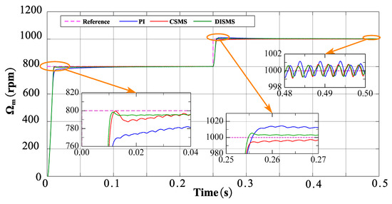
Figure 9.
Simulation results based on the CSMS and DISMS surfaces with NSMCEAL law, and PI controller: Ωm = 800 rpm to 1000 rpm and TL = 10 Nm.
Building on the previously utilized comprehensive evaluation approach, Table 4 and Figure 10 present an assessment and comparison of the control performance for four varieties of speed-robust controllers. In this evaluation, the maximum achievable score is set at 3.
Table 4.
Evaluating and comparing the performance indicators of controllers with the CSMS and DISMS surfaces.
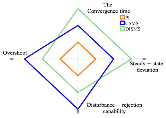
Figure 10.
Radar chart of the evaluations of the NSMCEAL law based on some surfaces and the PI controller.
In terms of the convergence time and disturbance rejection capability, the NSMCEAL law associated with the CSMS surface demonstrates a clear advantage. A more in-depth assessment of convergence rate factors and disturbance rejection robustness further reveals that the NSMCEAL control law on the CSMS-based surface exhibits significant and dominant superiority. Overall, the NSMCEAL law controller, when combined with the CSMS and DISMS surfaces, ranks highest due to its better overall performance in the radar chart. Figure 10 shows that the NSMCEAL law with the PI has the smallest overall performance.
4.2.3. Performance Analysis of Various Response Methods
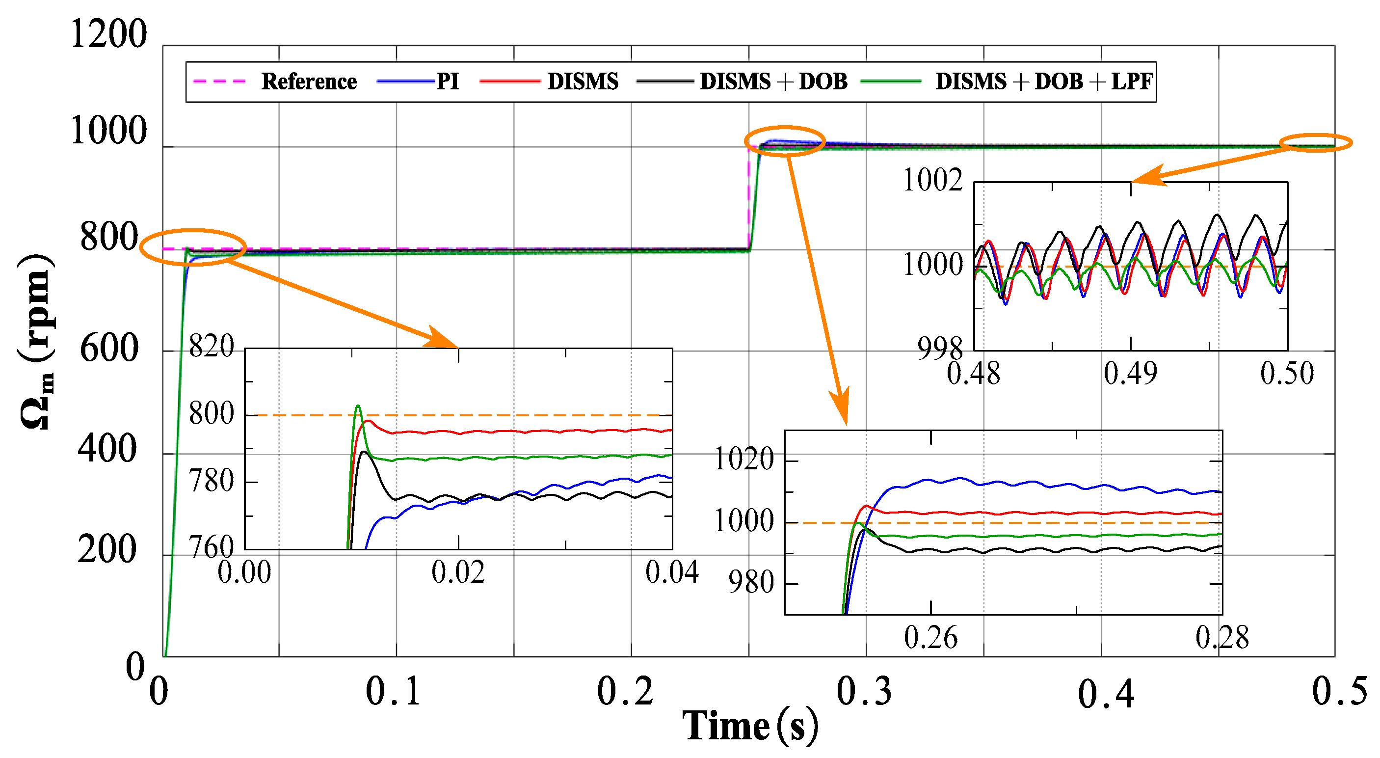
The fourth section presents a comparison of the dynamic performance of several systems. These include the system controlled by NSMCEAL + DISMS (DISMS), the one with NSMCEAL + DISMS + DOB (DISMS + DOB), the newly proposed NSMCEAL + DISMS + DOB + LPF (DISMS + DOB + LPF) in this paper, and the PI-controlled system. This comparison is made considering their relatively good performance characteristics.
Figure 11 demonstrates that the response speed of the DISMS, DISMS + DOB, and DISMS + DOB + LPF controllers during motor startup is faster than that of the PI controller. However, the maximum overshoot of the DISMS, DISMS + DOB, and DISMS + DOB + LPF controllers is higher than that of the PI controller. The response speed of the novel DISMS + DOB + LPF controller is superior to that of the DISMS, DISMS + DOB, and PI controllers when the load changes.
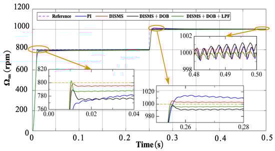
Figure 11.
Simulation result visualization: novel DIMS surface with NSMCEAL, DOB, LPF, and PI comparison: Ωm = 800 rpm to 1000 rpm and TL = 10 Nm.
For a comprehensive performance comparison, Table 5 and Figure 12 use an evaluation approach similar to the one employed previously. When considering key evaluation indices, such as steady-state deviation, overshoot, and disturbance rejection capability, the novel DISMS + DOB + LPF configuration outperforms the other alternatives.
Table 5.
Evaluating and comparing the performance indicators of controllers with the DISMS surface.
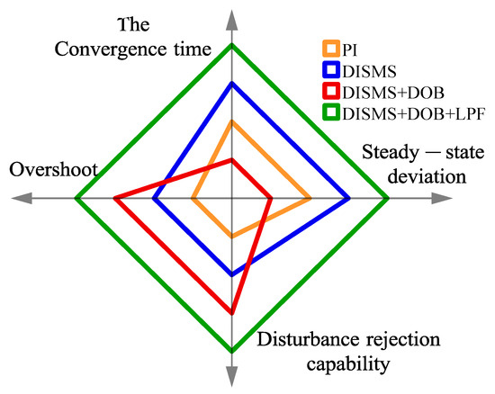
Figure 12.
The radar chart represents the evaluation of several controllers with better control performance.
In terms of the control system’s resilience against disruptions, the results from the novel DISMS + DOB + LPF setup clearly demonstrate that the proposed method achieves the desired performance levels. This is largely due to its ability to maintain stable speed even under challenging conditions.
4.2.4. Response Performance of Novel NSMCEAL + DISMS and Proposed NSMCEAL + DISMS + DOB + LPF
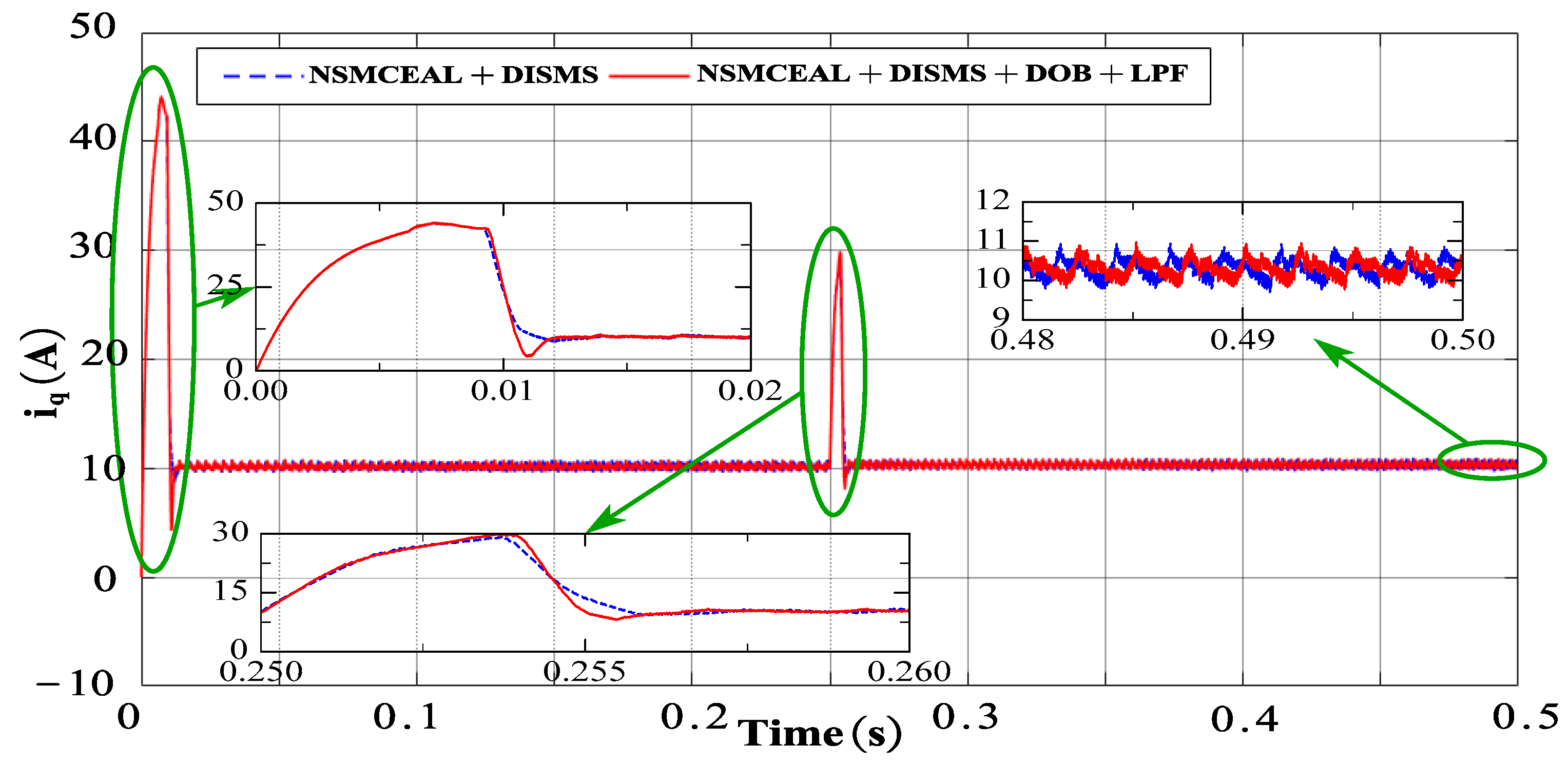
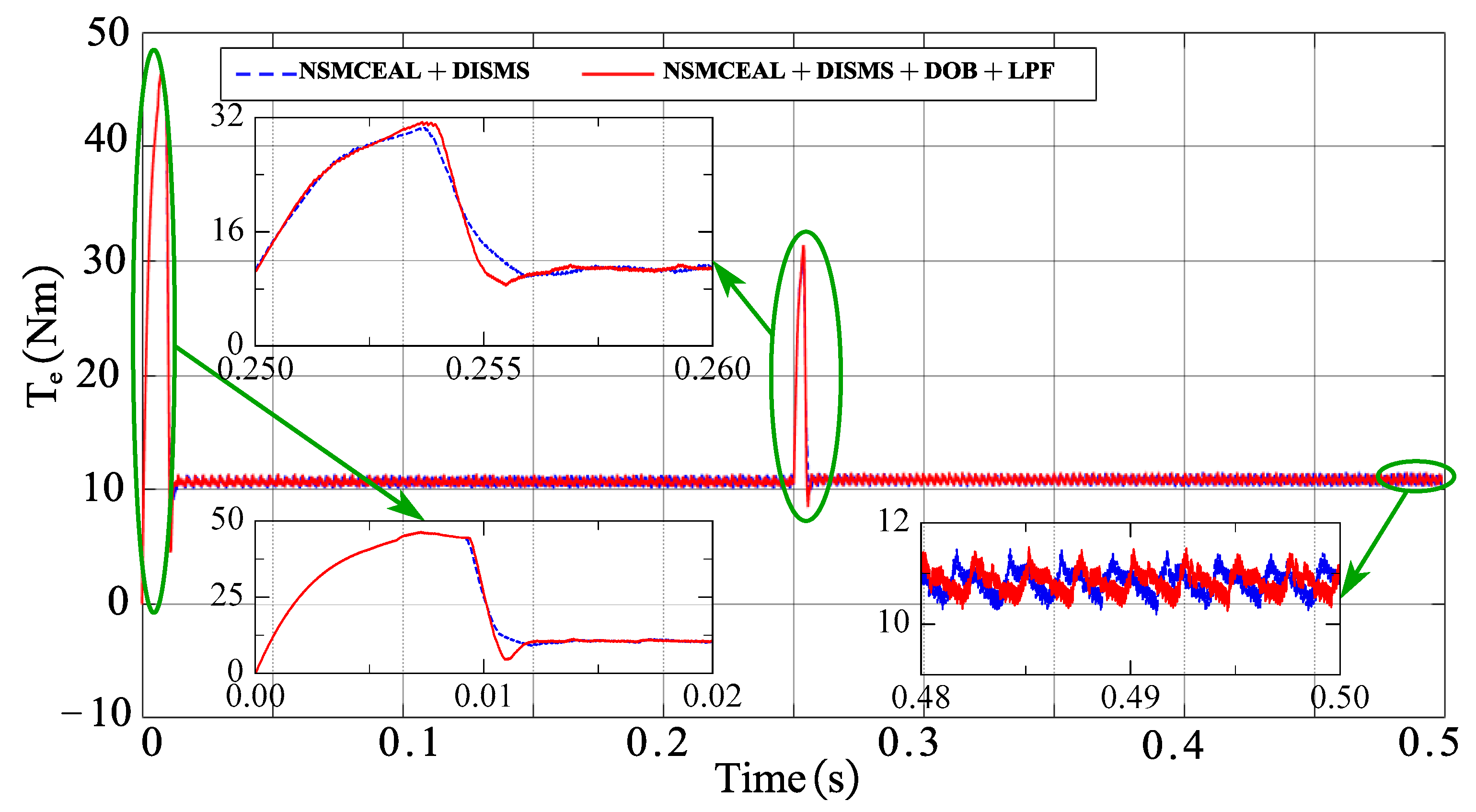
This section presents the simulation results for the novel NSMCEAL + DISMS combination and the newly proposed NSMCEAL + DISMS + DOB + LPF configuration. Figure 13, Figure 14, Figure 15 and Figure 16 show the speed curve, output current iq curve, output iA current curve, and torque curve of the novel NSMCEAL + DISMS and the proposed NSMCEAL + DISMS + DOB + LPF, respectively.
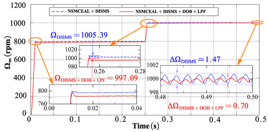
Figure 13.
Motor speed of the novel NSMCEAL + DISMS and proposed NSMCEAL + DISMS + DOB + LPF: Ωm = 800 rpm to 1000 rpm and TL = 10 Nm.

Figure 14.
Output iq current of the novel NSMCEAL + DISMS and proposed NSMCEAL + DISMS + DOB + LPF: Ωm = 800 rpm to 1000 rpm and TL = 10 Nm.
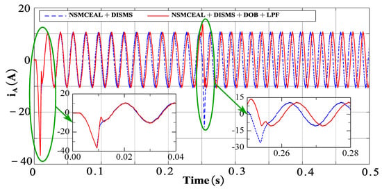
Figure 15.
Output iA current of the novel NSMCEAL + DISMS and proposed NSMCEAL + DISMS + DOB + LPF: Ωm = 800 rpm to 1000 rpm and TL = 10 Nm.
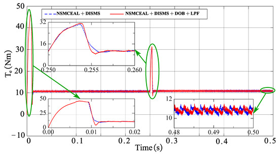
Figure 16.
Torque of the novel NSMCEAL + DISMS and proposed NSMCEAL + DISMS + DOB + LPF: Ωm = 800 rpm to 1000 rpm and TL = 10 Nm.
Additionally, the novel DISMS + DOB + LPF exhibits superior dynamic response speed. As shown in the radar chart, its overall performance, represented by the green section, is more favorable compared to other options, indicating its enhanced efficiency and responsiveness in dynamic scenarios.
The simulation results for the motor speed indicate that, compared to the new NSMCEAL + CSMS, the speed of the proposed steady-state deviation of NSMCEAL + DOB + LPF is 0.0276%, much lower than the novel NSMCEAL’s 0.04391%. In other cases, the parameters of the two controllers are equivalent.
5. Experimental Results
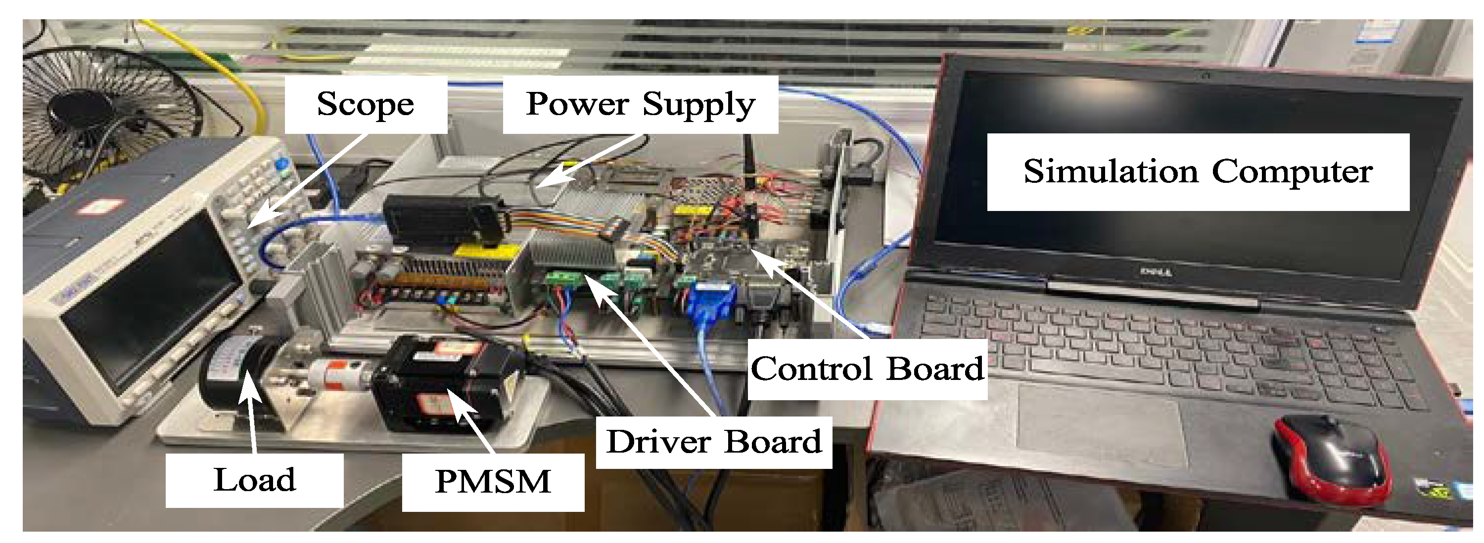
Figure 17 shows the construction of the experimental devices with a PMSM driver system. The system consists of a PMSM coupled with a Magnetic Damper (Model: MTB-06) providing an adjustable load torque range of 0.027–0.27 Nm. The motor is controlled using a TMS320F28335 DSP-based digital controller [25], which implements field-oriented control (FOC) for precise current and speed regulation. A three-phase FSBB30CH60 intelligent power module (IPM) serves as the inverter, operating at a switching frequency of 20 kHz with proper dead-time compensation. For data acquisition and real-time monitoring, the system utilizes an XDS100V3 debug probe connected via the JTAG interface, enabling parameter tuning and performance analysis. Experimental data are logged and processed using MATLAB/Simulink for graphical visualization and further analysis.

Figure 17.
The experiment platform.
The control algorithms are optimized based on the PMSM’s nominal parameters (provided in Table 6), ensuring stable and efficient operation under varying load conditions. Due to this limited range, the research team implemented fixed-step load adjustments (discrete torque levels) to evaluate the speed characteristics of the PMSM motor under controlled loading conditions. The effectiveness of the proposed control algorithm is verified through experimental results.
Table 6.
Experimental parameters of the PMSM motor.
In the following experiments, four SMC controller laws—CEAL, NSMC, ASMC, NSMCEAL, and PI—are designed and compared to verify the superiority of the proposed strategy. The controller gains and disturbance observer (DOB) parameters used in the experiment are listed in Table 7.
Table 7.
The gains of the SMC controller and the dob for experimental devices.
The DOB observer estimates the disturbance values using the following equations: The Q0 and R0 value is taken as the value from equation (39). The observer gain matrix L is calculated using Matlab, yielding the following new result:
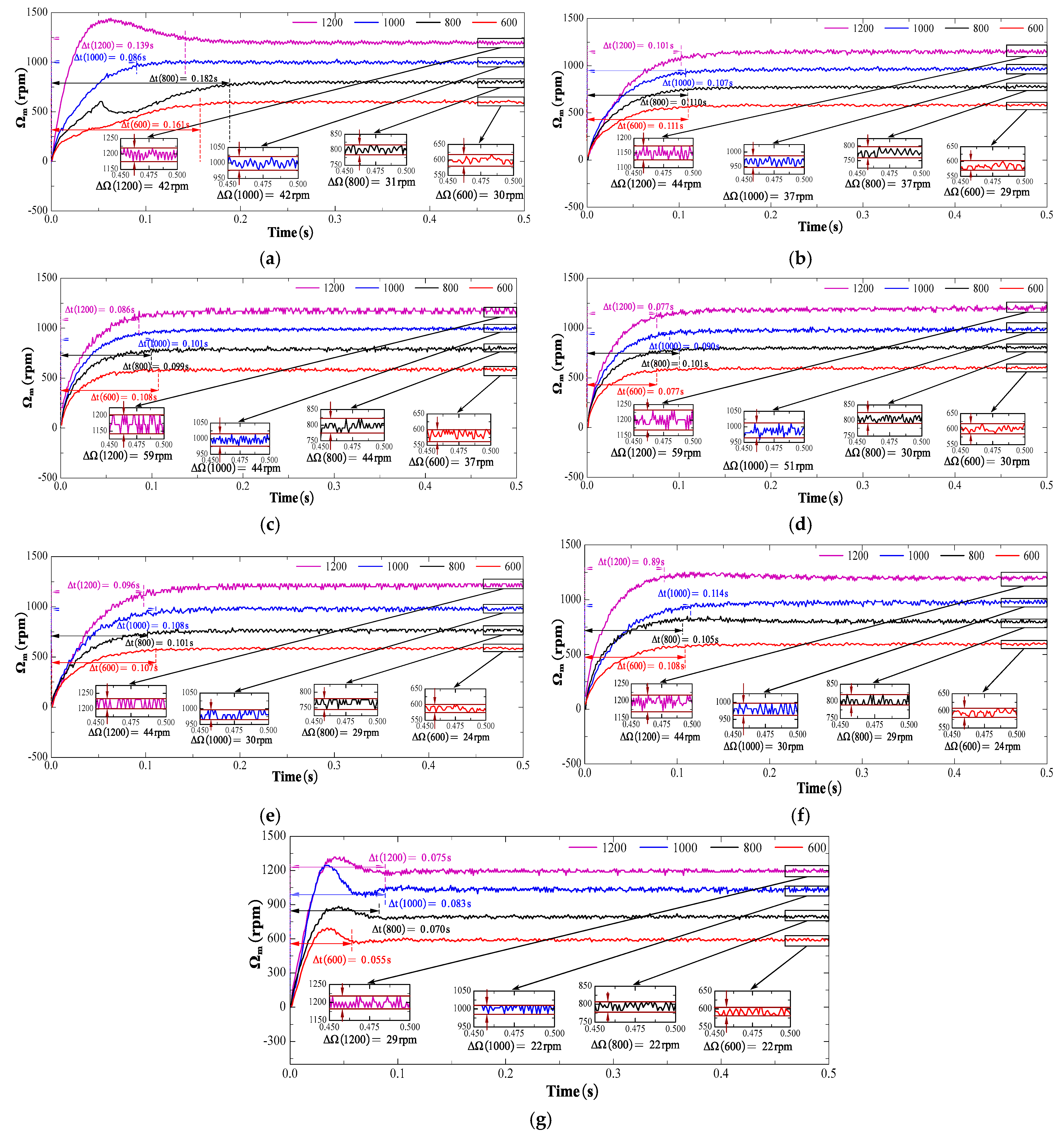
Figure 18 demonstrates the experiments in which the PMSM was tested across various speed levels, and the control performance was evaluated based on metrics, such as the startup time and speed error (TL = 0.057 Nm). Optimal compensation coefficients should be selected to ensure system stability and robustness while maximizing the disturbance-rejection capability. The Steady-State Error (SSE) is expressed as the ratio of the steady-state speed ripple to the rated speed of the PMSM drive and is calculated as follows:
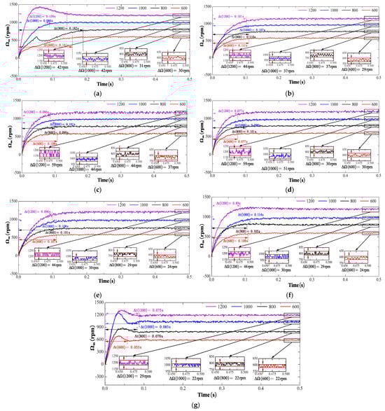
Figure 18.
Experimental speed results of the conventional sliding-mode surface with CEAL, NSMC, ASMC, NSMCEAL, and PI: (a) PI; (b) CEAL + CSMS; (c) NSMC + CSMS; (d) ASMC + CSMS; (e) NSMCEAL + CSMS; (f) NSMCEAL + DISMS; (g) NSMCEAL + DISMS + DOB + LPF.
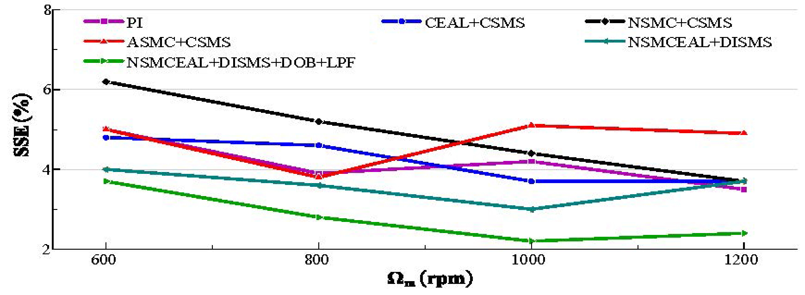
Figure 19 assesses the effectiveness of the designed control algorithm in comparison to conventional control methods. The speed varies among 600 rpm, 800 rpm, 1000 rpm, and 1200 rpm under a constant torque of 0.057 Nm. Ripple, which refers to unwanted oscillations in speed signals, is typically caused by disturbances or non-ideal system responses. The designed control algorithm achieves enhanced system robustness, with significant improvements in high-speed operation.
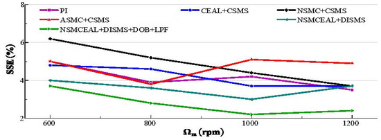
Figure 19.
The analysis of SSE for various speeds.
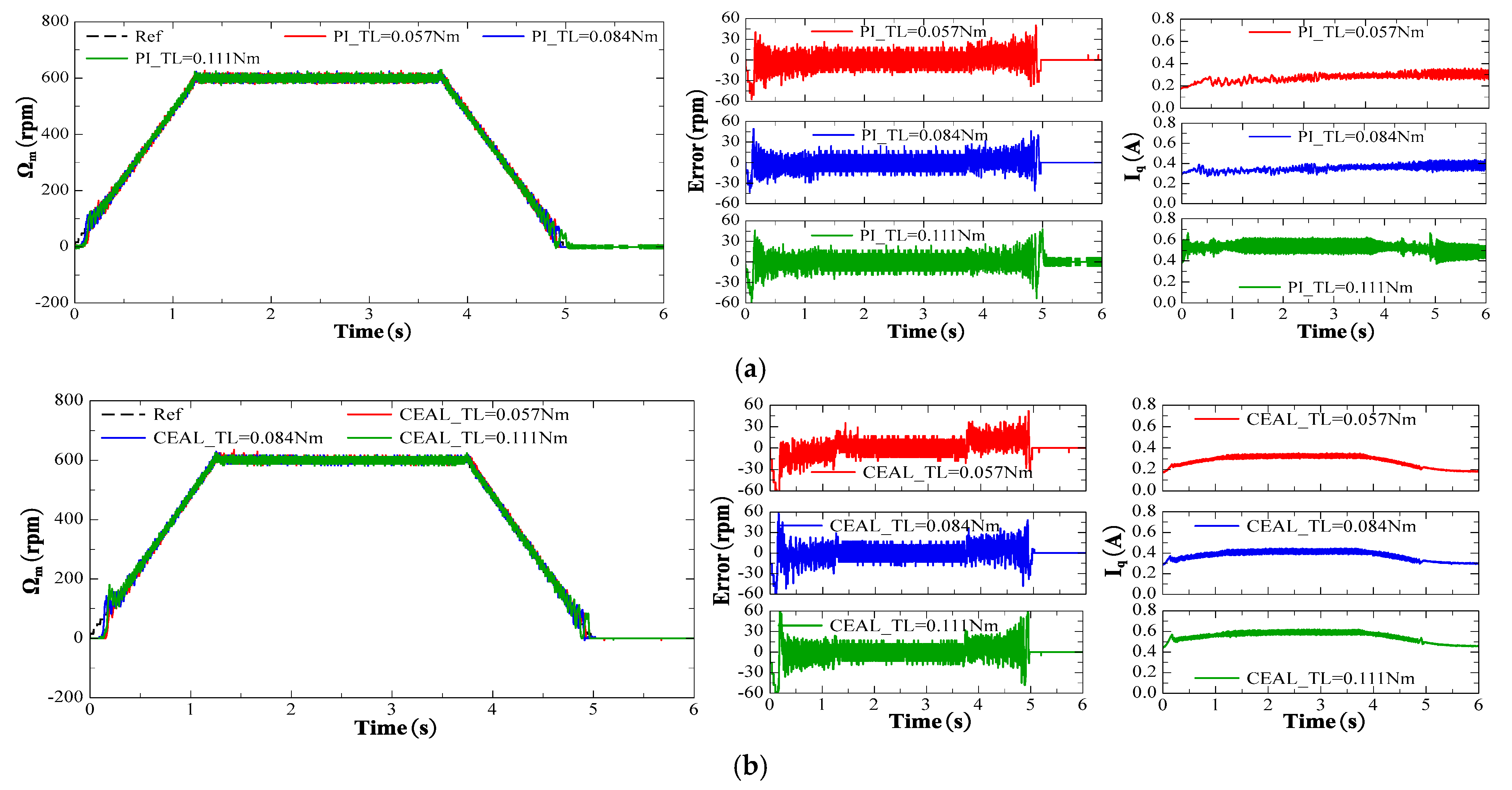
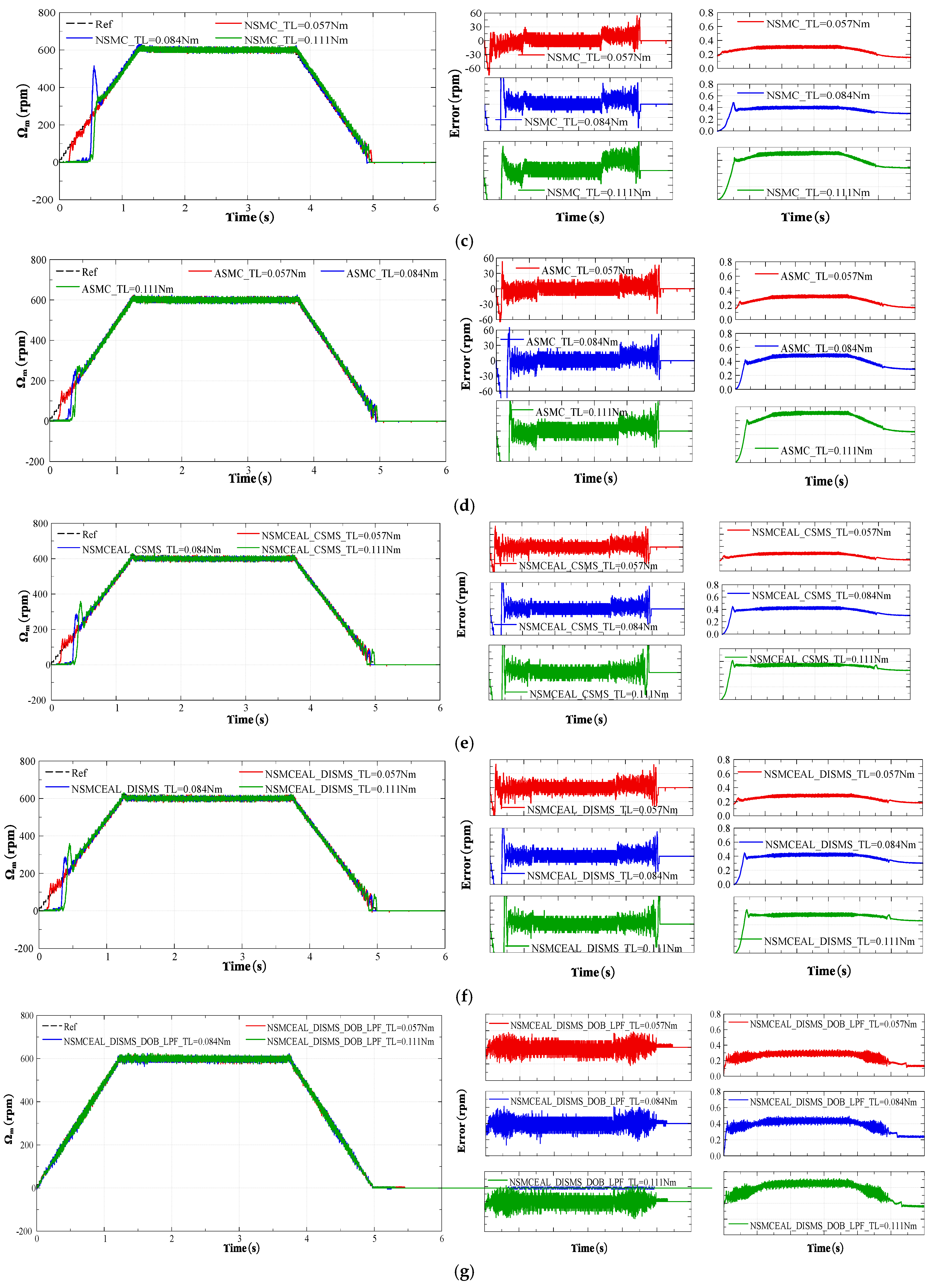
The same reference speed in the form of a ramp profile with different torque levels was used to compare various methods: PI control, CEAL, ASMC, NSMC, and NSMCEAL, as shown in Figure 20a–e, respectively. Figure 20e,f,g illustrate the NSMCEAL control method based on different sliding surfaces: CSMS, DISMS, and with the DOB + LPF (disturbance observer + low-pass filter).

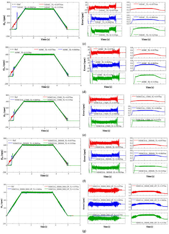
Figure 20.
Performance comparison of PI, CEAL, NSMC, ASMC, and the proposed NSMCEAL DISMS + DOB + LPF under a reference-speed ramp: (a) PI; (b) CEAL + CSMS; (c) NSMC + CSMS; (d) ASMC + CSMS; (e) NSMCEAL + CSMS; (f) NSMCEAL + DISMS; (g) NSMCEAL + DISMS + DOB + LPF.
The PI control exhibits significant speed errors when the speed changes, and torque variations lead to even larger oscillations, particularly in the iq current of the system, which shows substantial errors, especially under higher loads. The traditional SMC method demonstrates variations in the speed error, causing noticeable chattering, particularly when the torque increases. Additionally, there is an initial delay corresponding to different sliding-mode controllers, though the iq current error is smaller.
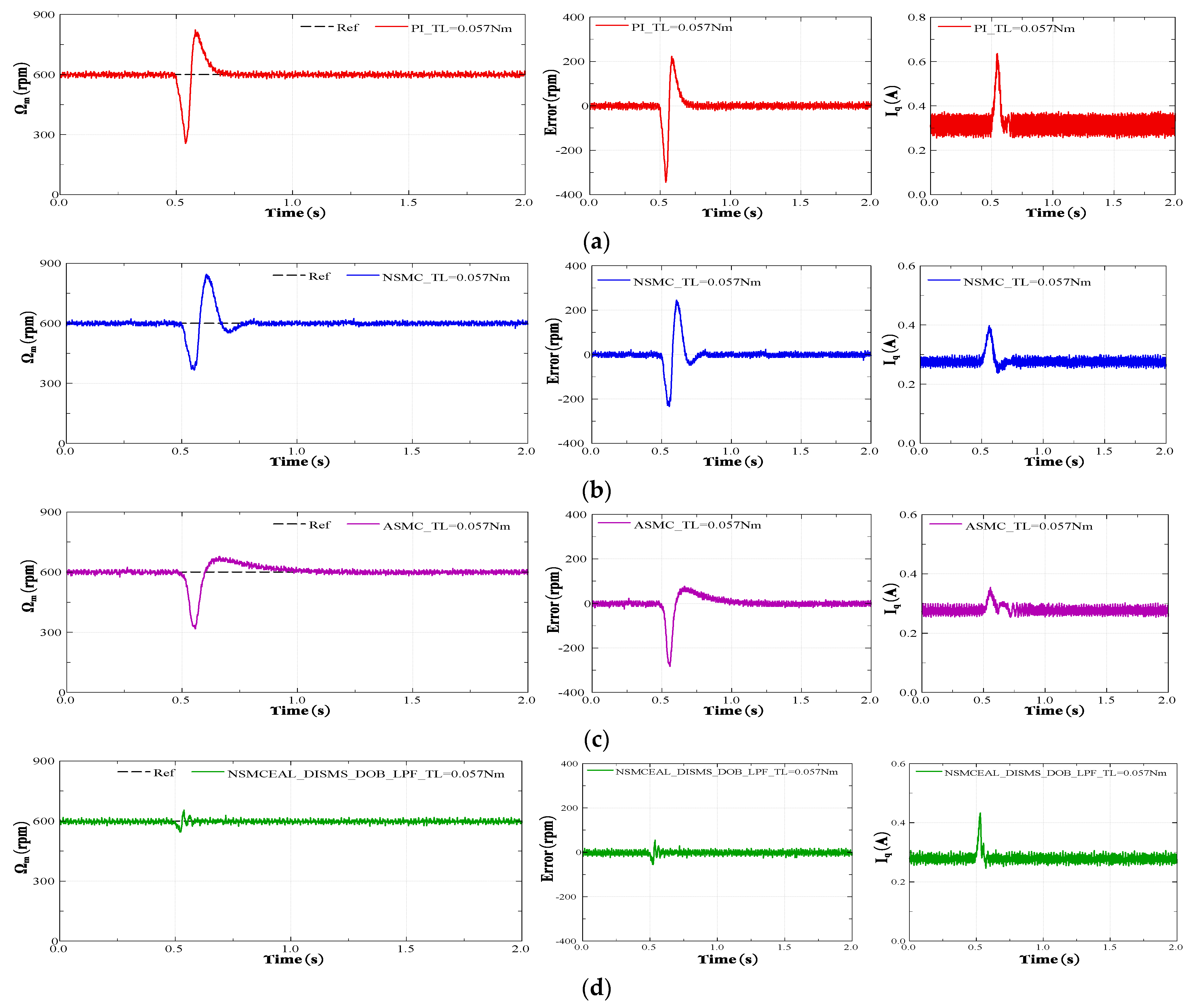
To assess the system’s robustness, an external load torque was abruptly applied to the motor shaft at t = 1 s. The subsequent variations in current and speed responses were monitored. The dynamic performance of the system using the PI controller, NSMC, ASMC, and the proposed method are illustrated in Figure 21. Results demonstrate the proposed method’s superior disturbance rejection capability compared to other approaches. The speed error is the largest with PI and NSMC when subjected to sudden impulse disturbances. ASMC exhibits smaller errors and lower overshoot. Meanwhile, the proposed new method is less affected by sudden impulses and achieves lower speed errors. However, the proposed method results in a higher iq current error compared to ASMC and NSMC, though it still performs better than the iq current error of the PI control.

Figure 21.
Speed response when the load torque suddenly occurs of PI, NSMC, ASMC, and the proposed NSMCEAL DISMS + DOB + LPF under a reference-speed ramp: (a) PI; (b) NSMC + CSMS; (c) ASMC + CSMS; (d) NSMCEAL + DISMS + DOB + LPF.
The NSMCEAL + DISMS + DOB + LPF method achieves superior performance by overcoming the drawbacks of other sliding-mode controllers while maintaining greater stability compared to PI control. Comparative performance of conventional and proposed control scheme is provided in Table 8.
Table 8.
Comparative performance of conventional and proposed control scheme.
6. Conclusions
This paper proposes an NSMCEAL + DISMS + DOB + LPF controller for PMSM systems. The controller is designed to enhance both the speed-tracking capability and disturbance rejection performance of the PMSM.
The NSMCEAL incorporates an adaptive reaching law that effectively reduces chattering phenomena and the reaching time compared to conventional SMC methods. Based on the proposed reaching law, the NSMCEAL controller has been specifically designed for the motor’s speed control loop.
Furthermore, the DOB + LPF combination successfully overcomes the inherent limitations of traditional sliding-mode control methods when handling varying load conditions. Experimental results validate that the integrated NSMCEAL + DISMS + DOB + LPF approach not only significantly reduces chattering but also achieves superior dynamic performance compared to conventional SMC.
While the current research focuses on improving the speed control loop, the impact of torque variations has not been fully evaluated. Therefore, torque fluctuation analysis will be addressed in future studies to further enhance the system’s performance.
Author Contributions
Conceptualization, T.T.T., J.Y. and J.Z.; methodology, T.T.T., J.Z. and L.L.; software, L.L.; validation, T.T.T., J.Y. and J.Z.; formal analysis, T.T.T. and J.Z.; investigation, T.T.T. and J.Y.; resources, T.T.T. and J.Y.; data curation, T.T.T. and J.Z.; writing—original draft preparation, T.T.T. and J.Y.; writing—review and editing, T.T.T., J.Y. and J.Z.; visualization, T.T.T. and J.Z.; supervision, J.Y. and L.L.; project administration, J.Y. and L.L.; funding acquisition, T.T.T. and J.Z. All authors have read and agreed to the published version of the manuscript.
Funding
This work was supported in part by the National Natural Science Foundation of China (52477071), in part by the Open Fund of the State Key Laboratory of High-Efficiency and High-Quality Conversion for Electric Power (No. 2024KF001).
Data Availability Statement
The data presented in this study are available on request from the corresponding author due to privacy reasons.
Conflicts of Interest
The authors declare no conflicts of interest.
References
- Huang, Z.; Zhou, D.; Wang, L.; Shen, Z.; Li, Y. A Review of Single-Stage Multiport Inverters for Multisource Applications. IEEE Trans. Power Electron. 2023, 38, 6566–6584. [Google Scholar] [CrossRef]
- Zhang, W.; Yang, Q.; Li, Y.; Lin, Z.; Yang, M. Temperature Dependence of Powder Cores Magnetic Properties for Medium-Frequency Applications. IEEE Trans. Magn. 2022, 58, 2300505. [Google Scholar] [CrossRef]
- Husain, I.; Ozpineci, B.; Islam, M.S.; Gurpinar, E.; Su, G.J.; Yu, W.; Chowdhury, S.; Xue, L.; Rahman, D.; Sahu, R. Electric Drive Technology Trends, Challenges, and Opportunities for Future Electric Vehicles. Proc. IEEE 2021, 109, 1039–1059. [Google Scholar] [CrossRef]
- Zhang, H.; Liu, W.; Chen, Z.; Jiao, N. An Overall System Delay Compensation Method for IPMSM Sensorless Drives in Rail Transit Applications. IEEE Trans. Power Electron. 2021, 36, 1316–1329. [Google Scholar]
- Hang, J.; Xia, M.; Ding, S.; Li, Y.; Sun, L.; Wang, Q. Research on Vector Control Strategy of Surface-Mounted Permanent Magnet Synchronous Machine Drive System with High-Resistance Connection. IEEE Trans. Power Electron. 2020, 35, 2023–2033. [Google Scholar]
- Tursini, M.; Parasiliti, F.; Zhang, D. Real-Time Gain Tuning of PI Controllers for High-Performance PMSM Drives. IEEE Trans. Ind. Appl. 2002, 38, 1018–1026. [Google Scholar]
- Maghfiroh, H.; Nizam, M. Improved LQR Control Using PSO Optimization and Kalman Filter Estimator. IEEE Access 2022, 10, 18330–18337. [Google Scholar]
- Systems, M. The Exact Model Matching of Linear Multivariable Systems. IEEE Trans. Automat. Contr. 1971, 17, 347–349. [Google Scholar]
- Tan, L.N.; Cong, T.P.; Cong, D.P. Neural Network Observers and Sensorless Robust Optimal Control for Partially Unknown PMSM with Disturbances and Saturating Voltages. IEEE Trans. Power Electron. 2021, 36, 12045–12056. [Google Scholar] [CrossRef]
- Shao, Y.; Yu, Y.; Chai, F.; Chen, T. A Two-Degree-of-Freedom Structure-Based Backstepping Observer for DC Error Suppression in Sensorless PMSM Drives. IEEE Trans. Ind. Electron. 2022, 69, 10846–10858. [Google Scholar] [CrossRef]
- Wang, Y.; Fang, S.; Hu, J. Active Disturbance Rejection Control Based on Deep Reinforcement Learning of PMSM for More Electric Aircraft. IEEE Trans. Power Electron. 2023, 38, 406–416. [Google Scholar] [CrossRef]
- Wang, C.; Zhu, Z.Q. Fuzzy Logic Speed Control of Permanent Magnet Synchronous Machine and Feedback Voltage Ripple Reduction in Flux-Weakening Operation Region. IEEE Trans. Ind. Appl. 2020, 56, 1505–1517. [Google Scholar] [CrossRef]
- Nguyen, T.T.; Tran, H.N.; Nguyen, T.H.; Jeon, J.W. Recurrent Neural Network-Based Robust Adaptive Model Predictive Speed Control for PMSM with Parameter Mismatch. IEEE Trans. Ind. Electron. 2023, 70, 6219–6228. [Google Scholar] [CrossRef]
- Lang, W.; Hu, Y.; Gong, C.; Zhang, X.; Xu, H.; Deng, J. Artificial Intelligence-Based Technique for Fault Detection and Diagnosis of EV Motors: A Review. IEEE Trans. Transp. Electrif. 2022, 8, 384–406. [Google Scholar] [CrossRef]
- Tang, B.; Lu, W.; Yan, B.; Lu, K.; Feng, J.; Guo, L. A Novel Position Speed Integrated Sliding Mode Variable Structure Controller for Position Control of PMSM. IEEE Trans. Ind. Electron. 2022, 69, 12621–12631. [Google Scholar] [CrossRef]
- Li, H.X.; Gatland, H.B.; Green, A.W. Fuzzy Variable Structure Control. IEEE Trans. Syst. Man. Cybern. Part B Cybern. 1997, 27, 306–312. [Google Scholar] [CrossRef]
- Zhang, Y.; Xu, D.; Huang, L. Generalized Multiple-Vector-Based Model Predictive Control for PMSM Drives. IEEE Trans. Ind. Electron. 2018, 65, 9356–9366. [Google Scholar] [CrossRef]
- Dai, C.; Guo, T.; Yang, J.; Li, S. A Disturbance Observer-Based Current-Constrained Controller for Speed Regulation of PMSM Systems Subject to Unmatched Disturbances. IEEE Trans. Ind. Electron. 2021, 68, 767–775. [Google Scholar] [CrossRef]
- Zhang, Y.; Jin, J.; Huang, L. Model-Free Predictive Current Control of PMSM Drives Based on Extended State Observer Using Ultralocal Model. IEEE Trans. Ind. Electron. 2021, 68, 993–1003. [Google Scholar]
- Feng, L.; Deng, M.; Xu, S.; Huang, D. Speed Regulation for PMSM Drives Based on a Novel Sliding Mode Controller. IEEE Access 2020, 8, 63577–63584. [Google Scholar] [CrossRef]
- Nguyen, T.H.; Nguyen, T.T.; Nguyen, V.Q.; Le, K.M.; Tran, H.N.; Jeon, J.W. An Adaptive Sliding-Mode Controller with a Modified Reduced-Order Proportional Integral Observer for Speed Regulation of a Permanent Magnet Synchronous Motor. IEEE Trans. Ind. Electron. 2022, 69, 7181–7191. [Google Scholar] [CrossRef]
- Liu, T.T.; Tan, Y.; Wu, G.; Wang, S.M. Simulation of PMSM Vector Control System Based on Matlab/Simulink. In Proceedings of the 2009 International Conference on Measuring Technology and Mechatronics Automation, ICMTMA, Zhangjiajie, China, 11–12 April 2009; Volume 2, pp. 343–346. [Google Scholar] [CrossRef]
- Suleimenov, K.; Do, T.D. Design and Analysis of a Generalized High-Order Disturbance Observer for PMSMs with a Fuzy-PI Speed Controller. IEEE Access 2022, 10, 42238–42246. [Google Scholar] [CrossRef]
- Seryasat, O.R.; Aliyari Shoorehdeli, M.; Honarvar, F.; Rahmani, A. Multi-Fault Diagnosis of Ball Bearing Using FFT, Wavelet Energy Entropy Mean and root Mean Square (RMS). In Proceedings of the 2010 IEEE International Conference on Systems, Man and Cybernetics, Istanbul, Turkey, 10–13 October 2010; pp. 4295–4299. [Google Scholar]
- Yang, J.; Zhou, J.; Zhou, H.; Yi, F.; Song, D.; Dong, M. High-Precision Harmonic Current Extraction for PMSM Based on Multiple Reference Frames Considering Speed Harmonics. IEEE Trans. Ind. Electron. 2023, 70, 9764–9776. [Google Scholar] [CrossRef]


Disclaimer/Publisher’s Note: The statements, opinions and data contained in all publications are solely those of the individual author(s) and contributor(s) and not of MDPI and/or the editor(s). MDPI and/or the editor(s) disclaim responsibility for any injury to people or property resulting from any ideas, methods, instructions or products referred to in the content. |
© 2025 by the authors. Licensee MDPI, Basel, Switzerland. This article is an open access article distributed under the terms and conditions of the Creative Commons Attribution (CC BY) license (https://creativecommons.org/licenses/by/4.0/).