Abstract
With the rapid development and widespread application of drones across various fields, drone recognition and classification at medium and long distances have become increasingly important yet challenging tasks. This paper proposes a novel network architecture called AECM-Net, which integrates an adaptive feature fusion (AF) module, an efficient channel attention (ECA), and a criss-cross attention (CCA) mechanism-enhanced multi-scale feature extraction module (MSC). The network employs both Mel-frequency cepstral coefficients (MFCCs) and Gammatone cepstral coefficients (GFCC) as input features, utilizing the AF module to adaptively adjust fusion weights of different feature maps while incorporating ECA channel attention to emphasize key channel features and CCA mechanism to capture long-range dependencies. To validate our approach, we construct a comprehensive dataset containing various drone models within a 50-m range and conduct extensive experiments. The experimental results demonstrate that our proposed AECM-Net achieves superior classification performance with an average accuracy of 95.2% within the 50-m range. These findings suggest that our proposed architecture effectively addresses the challenges of medium and long-range drone acoustic signal recognition through its innovative feature fusion and enhancement mechanisms.
1. Introduction
In recent years, with the increasing market demand and technological advancement, drones have been widely applied across various industries. In agriculture, monitoring and spraying tasks have been performed by drones, optimizing the efficiency of pesticide and fertilizer application while detecting pests and diseases [1]. In construction, remote inspection of hard-to-reach or dangerous areas has been enabled by drones’ compact size and maneuverability, including regular inspections of bridges, dams, and high-rise buildings [2]. Moreover, significant roles in military applications have been demonstrated by drones, as evidenced by recent events in Ukraine [3].
However, while social progress has been promoted by drones, various security risks have also been posed. Drugs may be transported or explosives may be carried by drones that could threaten human life [4]. In recent years, “illegal flying” incidents due to a lack of safety awareness have become increasingly common, posing major threats to public safety. Normal civil aviation operations have been affected by drones violating flight altitude restrictions [5]. Therefore, developing intelligent and efficient drone detection technology is imperative to address security issues arising from unregulated drone development.
Current drone identification technologies have been categorized into radar detection, video image detection, radiofrequency signal detection, and acoustic detection methods [6]. Due to the drones’ small size, traditional radar systems have encountered difficulties in detection. A 90% recognition rate in experimental conditions has been achieved using Doppler radar sensors for automatic detection and classification of micro-drones [7]. However, radar detection equipment remains expensive, and numerous restrictions are often faced in radar deployment. Drone presence was determined by analyzing camera-captured images using visual image-based detection methods. However, this method’s effectiveness has been limited by environmental dependence and the inability to detect drones at night or when obscured [8]. In RF signal-based drone identification, RF signal identification tags have been utilized for detection and tracking [9]. However, interference from other wireless devices or high-frequency power sources has been found to affect this method. Unique advantages have been offered by acoustic detection, overcoming certain limitations of visual, RF, and radar methods, with benefits including low equipment cost, easy miniaturization and integration, and compatibility with other methods [10].
Acoustic-signal-based drone detection is essentially a sound event detection (SED) technology, which typically involves extracting features from acoustic signals, followed by classifying these features using acoustic models to identify and determine the types of sounds [11,12]. Before deep learning was applied to sound signal recognition, various machine learning methods had been well-established for acoustic classification, including support vector machines (SVM) [13], Gaussian mixture models (GMM) [14], and hidden Markov models (HMM) [15]. Extensive studies in acoustic recognition have been conducted using these models. Environmental sound classification tasks have been completed by extracting MFCC features combined with GMM models [16]. Breath sound classification has been achieved using cepstral features and SVM [17]. Heart sound abnormalities have been identified through MFCC features combined with HMM classifiers [18]. Heart sound recognition has been accomplished by extracting short-time energy features combined with SVM [19]. Voiced and unvoiced speech signals have been distinguished by extracting short-time zero-crossing rate features combined with classifiers like SVM [20]. While good performance has been demonstrated by these traditional acoustic recognition models on small datasets, with high computational efficiency and strong interpretability, limitations have been found in handling large-scale data and capturing long-term dependencies.
The concept of deep learning was introduced in 2006 when it was demonstrated that neural networks with multiple hidden layer structures could better extract deep abstract features of targets [21]. Since then, deep learning techniques have been increasingly incorporated into sound signal recognition research, where superior recognition accuracy has been achieved through excellent feature extraction capabilities. Deep learning algorithms were first combined with restricted Boltzmann machines in acoustic signal recognition research, where superior recognition performance compared to traditional algorithms was achieved [22].
Katta et al. benchmarked multiple audio-based deep learning models for UAV detection and identification, comparing various architectures including CNNs, RNNs, and hybrid models, evaluating their robustness and performance across different noise environments, and providing practical guidelines for designing efficient acoustic-based drone monitoring systems [23]. The recognition effects of CNN and SVM classifiers have been compared using MFCC features from drone acoustic signals, where the potential of deep learning technology in improving recognition accuracy was proven [24]. A method combining Gammatone GFCC features and sound signal spectrograms with the AlexNet network has been proposed, providing important evidence for the acoustic diagnosis of typical mechanical faults in power transformers [25]. A drone detection method based on short-time Fourier transform (STFT) features and CNN has been developed [26].
The feature fusion has been recognized as a powerful technique for integrating features from different sources or processing stages to extract richer and more valuable information, significantly enhancing machine learning model performance. Chroma features have been introduced and concatenated with commonly used Log-Mel spectrograms and MFCCs to enrich single feature representation capabilities [27]. MFCC and time-domain features (MFCCT) have been combined, integrating the effectiveness of both to improve text-independent speaker recognition system accuracy [28]. Three fusion strategies at the feature level have been implemented: concatenation of prenormalized features, the merging of normalized features, and the product of face and voice feature [29].
Low-frequency and timbre information have been extracted from bird songs using Mel and Sincnet filters. Two feature sets have been fused using a dual-feature fusion module. These methods have been shown to effectively improve feature expression and classification accuracy while suppressing noise and maintaining generalization ability [30]. An SE-TDNN-LSTM speaker recognition model based on residual connections has been proposed, where SE-TDNN modules are first used to extract local features of speech signals, then residual connections are utilized for feature information sharing, passing learned multi-scale features to LSTM-TDNN modules to capture long-term dependencies and extract higher-level features, completing global contextual information modeling [31]. The combination of the five-layer CA attention mechanism with the GoogLeNet algorithm has been proposed to improve new algorithm accuracy [32].
In drone acoustic recognition tasks, single features often struggle to comprehensively represent acoustic characteristics. Although MFCC and GFCC features each possess distinct advantages, effectively integrating these complementary features remains a significant challenge. Simple feature concatenation methods fail to adequately utilize the varying importance of different features and tend to introduce redundant information. To address this challenge, we propose an adaptive feature fusion (AF) module. This innovative module incorporates self-calibration operations to adaptively adjust fusion weights based on feature significance, thereby emphasizing crucial feature information while suppressing redundant features. Furthermore, to enhance feature expressiveness, we introduce the efficient channel attention (ECA) mechanism following the AF module. This mechanism models the importance of different channel features, enabling the network to highlight key channel characteristics and improve model performance.
Considering that traditional convolution operations’ limited receptive field constrains the modeling of long-range dependencies, we embed a criss-cross attention (CCA) module after each multi-scale feature extraction module. The CCA module establishes correlations between different positions in feature maps, effectively capturing long-range dependencies and significantly enhancing feature representation capabilities [33]. Based on these considerations, we propose AECM-Net, a network architecture for high-precision acoustic recognition of drones at medium and long distances. This network achieves comprehensive and efficient modeling of drone acoustic features through adaptive feature fusion and multi-level attention enhancement. The main contributions of this paper are as follows:
- Construction of an audio dataset containing four types of drones within a range of 0–50 m. This dataset enriches the sample diversity of medium to long-distance drone acoustic signals, providing strong support for studying drone recognition in complex environments.
- Proposal of an innovative feature fusion method: adaptive dual-feature fusion module (AF) combined with ECA channel attention mechanism. The AF module effectively highlights strong expressive features while suppressing redundant or noisy features through adaptive weight adjustment of different features. The introduction of the ECA channel attention mechanism after the AF module further enhances the representation capability of fused features, enabling the network to focus more on key channel features.
- Integration of a CCA cross-attention mechanism after each multi-scale feature extraction module in the AECM-Net network. The CCA attention mechanism improves the speed and accuracy of information transmission between internal modules, effectively enhancing the network’s recognition accuracy.
The rest of this paper is organized as follows. Section 2 presents the details of AECM-Net architecture, including the feature extraction process, the innovative AF feature fusion module, the ECA attention mechanism, and the CCA-MSC feature enhancement algorithm. Section 3 presents experimental results and analysis, including dataset description, comparative experiments of different fusion methods, ablation studies, and performance comparison with other state-of-the-art methods. Section 4 concludes the paper by summarizing the main findings and suggesting future research directions.
2. The Proposed Method
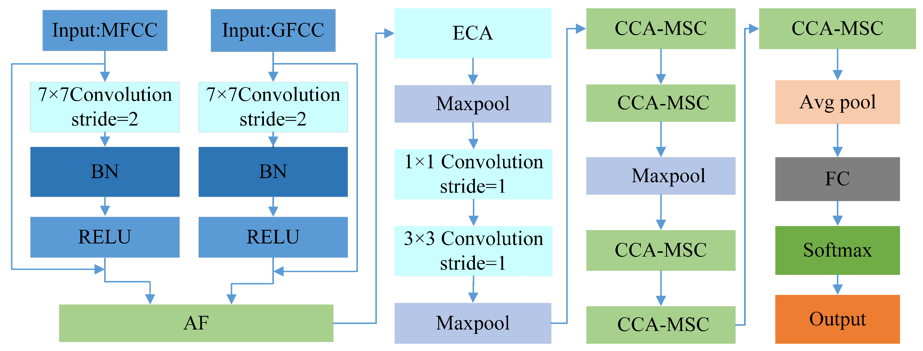
The acoustic model employed in this paper is a deep-learning-based acoustic recognition model. Specifically, we propose a novel network architecture, AECM-Net, with innovations manifested in both feature fusion and feature enhancement aspects. The network utilizes MFCC and GFCC features as input features. In terms of feature fusion, we introduce an adaptive feature fusion module, implemented in the intermediate network layers, which effectively integrates the advantages of both MFCC and GFCC feature maps obtained after feature extraction modules while adaptively adjusting fusion feature weights. To further enhance the representation capability of fused features, we incorporate an ECA (efficient channel attention) mechanism to emphasize the importance of key channel features. Regarding feature enhancement, we embed the CCA (criss-cross attention) mechanism into each multi-scale feature extraction module. The CCA mechanism effectively captures long-range dependencies and significantly enhances feature map representation capability.
The network architecture adopts a dual-input branch design, receiving MFCC and GFCC features separately. Both branches initially pass through residual-connection-based feature extraction modules to generate two types of feature maps. These feature maps are then input into the AF module for fusion. The fused features undergo the ECA channel attention mechanism, further highlighting the channel importance of the fused features. The feature maps processed by the ECA mechanism sequentially pass through max pooling, 1 × 1 convolution, and 3 × 3 convolution operations (all with stride 1), followed by another max pooling layer. Subsequently, they enter a series of CCA-MSC modules. The multi-scale feature extraction module (MSC) primarily aims to extract features at different scales and abstraction levels from feature maps, enhancing the network’s comprehension and representation capabilities of targets. By introducing the cross-channel attention mechanism in the MSC modules, the feature expression capability is effectively enhanced. After feature enhancement through the CCA mechanism, the network completes final feature processing and classification output through average pooling, fully connected layers, and Softmax activation function. The network structure is illustrated in Figure 1.
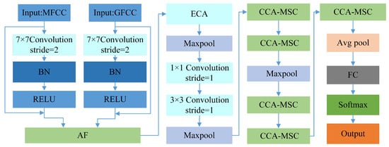
Figure 1.
The overall architecture of the AECM-Net Network.
2.1. Input Features
In drone acoustic signal recognition research, feature selection is crucial for recognition performance. As a classical acoustic feature, MFCC has demonstrated its effectiveness in drone sound recognition tasks across multiple studies [34]. MFCC effectively captures the spectral characteristics of drone sounds and shows excellent performance in multi-type drone classification.
On the other hand, GFCC features, based on the human auditory model, show unique advantages in certain scenarios. Research indicates that GFCC exhibits better robustness compared to MFCC in low signal-to-noise ratio environments, which is particularly significant for long-range drone recognition [35].
Considering the respective advantages of MFCC and GFCC, this paper chooses to extract both features simultaneously, fully utilizing their complementarity through subsequent feature fusion to enhance recognition performance. Next, we will provide a detailed introduction to the extraction process of both MFCC and GFCC features.
2.1.1. MFCC Feature Extraction
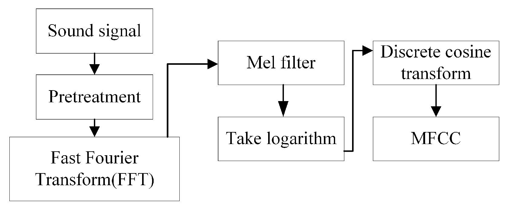
As shown in Figure 2, the preprocessing stage includes pre-emphasis, framing, and windowing of the acoustic signal. Below is a detailed description of the MFCC feature extraction process.
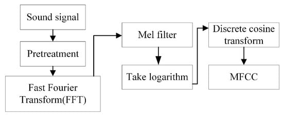
Figure 2.
The MFCC feature extraction.
Step 1: Pre-emphasis
The horn sounds collected by microphones at intersections are significantly affected by noise. Pre-emphasis can improve the signal-to-noise ratio as follows:
where the pre-emphasis coefficient is , represents the current audio signal, represents the previous audio sample, and is the signal after pre-emphasis.
Step 2: Framing
Since audio signals continuously change over time, making them difficult to analyze, the sound is divided into multiple frames, after which the signal can be considered stationary. Frameshift is introduced to smooth the transitions between adjacent frames. In this paper, the frame length is 2048 with a frameshift of 512, resulting in a frame duration of approximately 0.046 seconds at a 44.1 kHz sampling rate.
Step 3: Windowing
A window function is a finite-length signal in the time domain used to truncate infinite-length signals, enabling FFT to process only the truncated signal. Window functions reduce spectral leakage from signal truncation and improve spectral analysis accuracy. Common window functions include rectangular, Hanning, flat-top, Hamming, and Blackman windows. The Hanning window, offering balanced performance, features rapid side-lobe attenuation and effectively suppresses interference from frequency components far from the main lobe while maintaining good frequency resolution with its narrow main lobe width. Due to these characteristics, the Hanning window is widely used in MFCC feature extraction. The Hanning window is mathematically expressed as:
where n is the sample index, M is the window length (number of samples), and is the window function.
Step 4: Fast Fourier Transform (FFT)
The purpose of this step is to transform the framed and windowed signal into the frequency domain. While signal characteristics are difficult to discern in the time domain, Fourier transformation provides richer information about the acoustic signal. The FFT output is expressed as:
where is the original time-domain signal, N is the total number of samples, k is the frequency index, and n is the sample index. After the Fourier transform, the absolute value of the signal is taken and squared to obtain the power spectrum.
Step 5: Mel Filter Bank
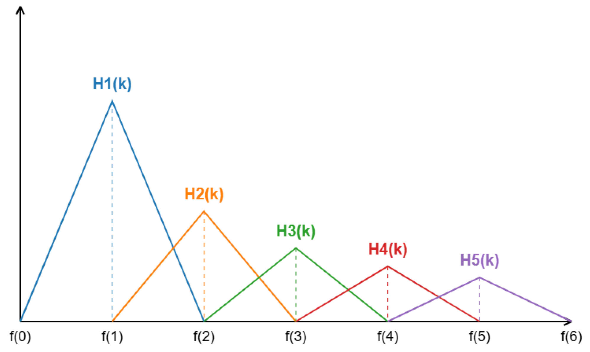
After obtaining the energy spectrum through FFT in Step 4, a Mel filter bank needs to be constructed and dot-multiplied with the energy spectrum. This aims to convert the energy spectrum into a Mel spectrum that better approximates the human auditory perception characteristics. The constructed Mel frequency filter bank is shown in Figure 3.
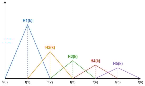
Figure 3.
The Mel filter bank.
The frequency response of the triangular filter is defined as follows
where is the response of the mth filter at frequency k, m is the filter index, and k is the frequency bin index corresponding to frequency points in the FFT output. , , and represent the center frequencies of the current, previous, and next filters, respectively.
Step 6: Take logarithm
The human ear exhibits remarkable sensitivity to small increases in sound intensity at low volumes, capable of detecting subtle changes. However, when sound intensity reaches higher levels, even significant changes become less perceptible to human hearing. This logarithmic perception of sound intensity is known as the logarithmic characteristic of human auditory perception. Therefore, the logarithmic operation is applied to better match the signal processing with this logarithmic nature of human hearing.
where is the power spectrum of the FFT, is the response of the mth Mel filter at frequency k, N is the number of FFT points, and M is the number of Mel filters (typically ranging from 20 to 40).
Step 7: Discrete Cosine Transform (DCT)
The purpose of this step is to redistribute the data and distinguish redundant information. After the transform, most of the signal data become concentrated in the low-frequency region, and thus, typically only the first portion of the transformed data needs to be retained.
where represents the nth MFCC coefficient, is the logarithmic Mel band energy of the mth filter, M is the number of Mel filters, and n is the number of MFCC coefficients we wish to retain (typically between 12 and 20).
2.1.2. GFCC Feature Extraction
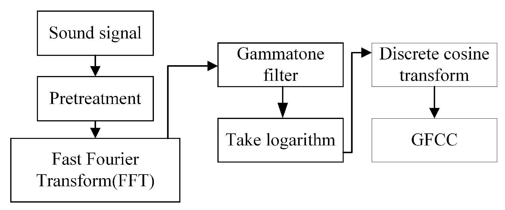
As shown in Figure 4 above, the GFCC feature extraction process is similar to that of MFCC feature extraction, with the main difference being the filter bank used. The Gammatone filter used in this process is described below.
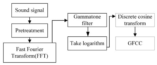
Figure 4.
The GFCC feature extraction.
The continuous impulse response of the Gammatone filter is as follows:
where a is the amplitude factor of the filter; represents time; is the filter order that simulates human auditory perception; is the phase factor, typically set to ; is the center frequency corresponding to the ith filter; is the bandwidth of the ith filter, which determines the decay rate of the impulse response; and represents the Equivalent Rectangular Bandwidth, and its relationship with frequency f is as follows:
where is the number of filters, determined by the frequency coverage range of the entire filter bank.
where and represent the lower and upper frequency bounds, respectively, and denotes the ceiling function.
In the Gammatone filter bank, the center frequencies of the filters are equally spaced in the ERB domain. Therefore, after determining the number of filters N based on the frequency coverage range of the filter bank, we have the following:
Based on (11), the center frequency corresponding to the ith filter can be calculated using Equation (9).
2.2. Feature Extraction Module Based on Residual Connection
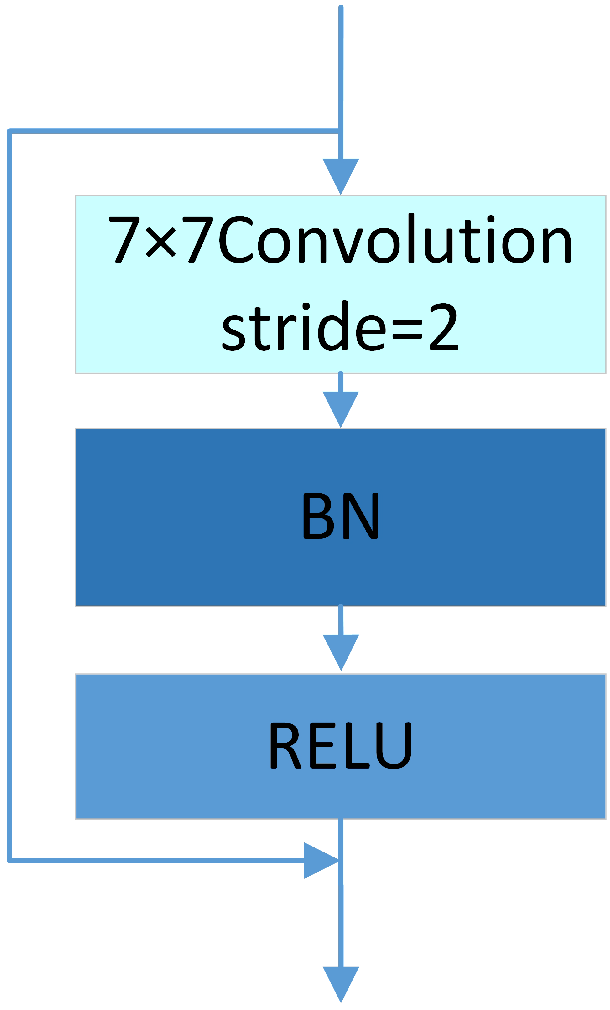
The combination of convolutional layers and Batch Normalization (BN) layers is a very common and effective feature extraction module design. The BN layer normalizes feature maps for each batch, making their mean close to 0 and variance close to 1. This helps accelerate network convergence and improve training stability.
As the number of neural network layers increases, the network becomes deeper, allowing it to learn richer features. However, during training, data not only need to propagate forward but also require backpropagation of errors from the final layer to earlier layers. If there are too many neural network layers, the gradient can easily vanish when passing through activation functions, a phenomenon known as gradient vanishing. Therefore, this paper introduces a residual structure in the dual feature fusion module. Figure 5 shows the feature extraction module based on residual connection. Figure 6 illustrates the residual structure diagram.
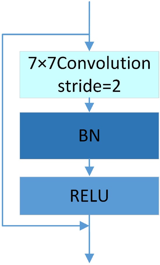
Figure 5.
Feature extraction module based on residual connections.
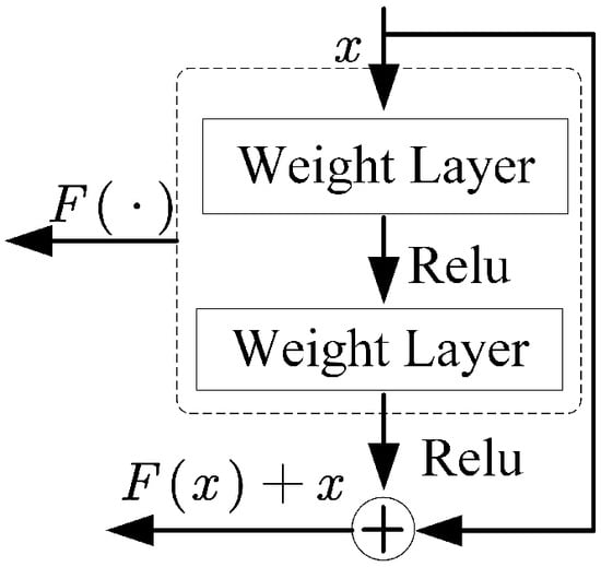
Figure 6.
Residual structure diagram.
2.3. Adaptive Feature Fusion (AF) Module
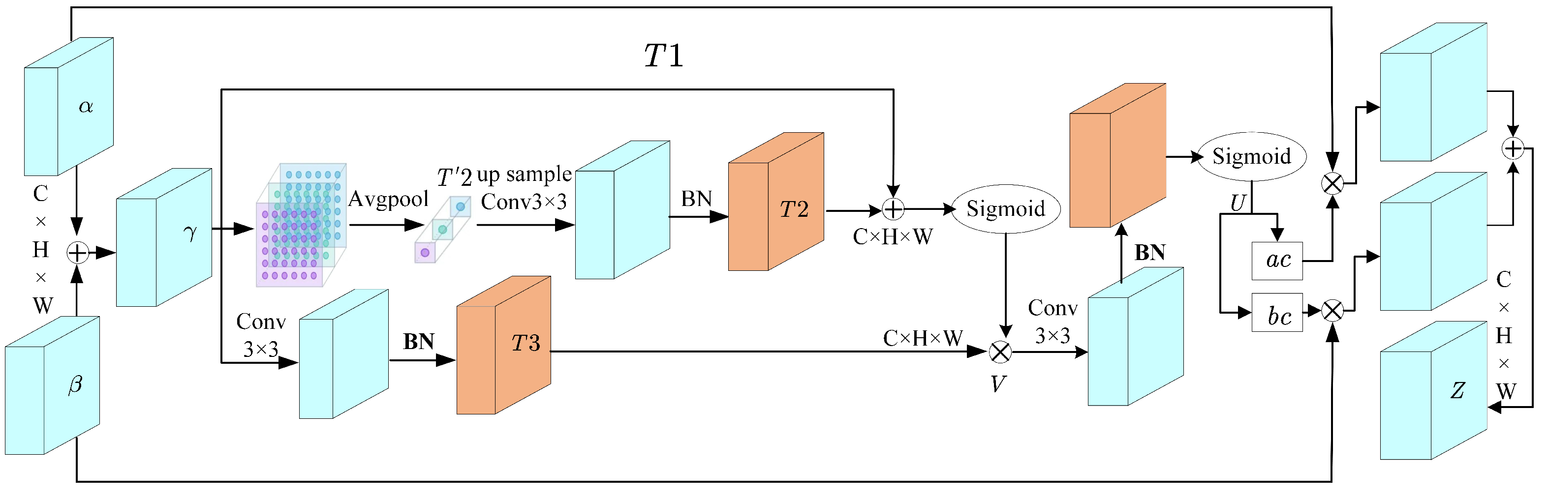
To effectively integrate the complementary acoustic features of MFCC and GFCC, this paper innovatively proposes an adaptive feature (AF) fusion module. A key characteristic of the AF module is its self-calibration mechanism, which adaptively adjusts the weights of different feature maps. In convolutional neural networks, feature maps in intermediate layers typically contain higher-level, more abstract feature representations. These feature maps may exhibit certain correlations and complementary relationships. By fusing intermediate-layer features through the AF module, these correlations and complementarities can be utilized to improve the quality of feature representation. Furthermore, the self-calibrating weights can emphasize important features while suppressing noise or redundant information, helping enhance the discriminative power of intermediate-layer features. Figure 7 illustrates the internal structure of the AF module.

Figure 7.
AF module structure diagram.
According to Figure 7, the steps of the AF module are as follows:
Add the two feature maps and element-wise after convolution pooling to obtain feature map .
The input is processed in three branches, where the first branch preserves the original input features . The second branch applies average pooling with a 2 × 2 filter and stride of 2 to obtain , then maps it back to the original feature space through upsampling to obtain :
where BN represents the normalization operation, is a predefined set of filter banks, Up denotes bilinear interpolation upsampling, and ∗ denotes the convolution operation. The third branch directly performs the convolution operation followed by batch normalization on to obtain
The self-calibration operation is then performed on the three branches to obtain V:
where is the activation function, ⊙ represents element-wise multiplication, and serves as the residual, which helps form self-calibration weight information.
After the self-calibration result V goes through convolution and Sigmoid function activation, it outputs U is given as:
The output U is mapped to the fusion weight dimension to calculate the fusion weights:
The final output Z, which is the fused feature, is:
where does not represent traditional matrix multiplication, but rather element-wise multiplication.
Below, we will explain the principles of adaptive fusion based on the internal structure of the AF module:
- Multi-scale Feature Extraction:
- Fusion module first performs multi-scale feature extraction on the initial fusion feature map, generating three feature maps (, , and ) at different scales through average pooling and convolution operations.
- This step extracts features from different receptive fields and resolutions, capturing different levels of feature information.
- Gate Signal Generation:
- Next, the fusion module adds and the resized , then generates a gate signal through a sigmoid activation function.
- This gate signal regulates the degree of fusion between different scale features, acting as an adaptive switch.
- The sigmoid function maps the sum to values between 0 and 1, serving as fusion weight coefficients.
- Selective Feature Fusion:
- The fusion module performs element-wise multiplication between the gate signal and to obtain feature map V. Through this operation, the gate signal selectively modulates features in .
- This step performs adaptive feature selection and modulation on through the gate signal, resulting in a new feature map V where important features are emphasized and minor features are suppressed.
- Fusion Weight Learning:
- To further optimize the fusion process, the fusion module performs convolution and sigmoid operations on V to obtain fusion weights (U). These fusion weights act as an adaptive fusion strategy, guiding the weight distribution of different features during fusion.
- Weighted Fusion:
- Finally, the fusion module uses the fusion weights (U) to perform weighted fusion of the original two feature maps ( and ), obtaining the final fused feature map (Z).
- This step adaptively fuses features from different sources according to their importance, resulting in a feature representation with enhanced discriminative power and complementarity.
2.4. ECA Attention Mechanism
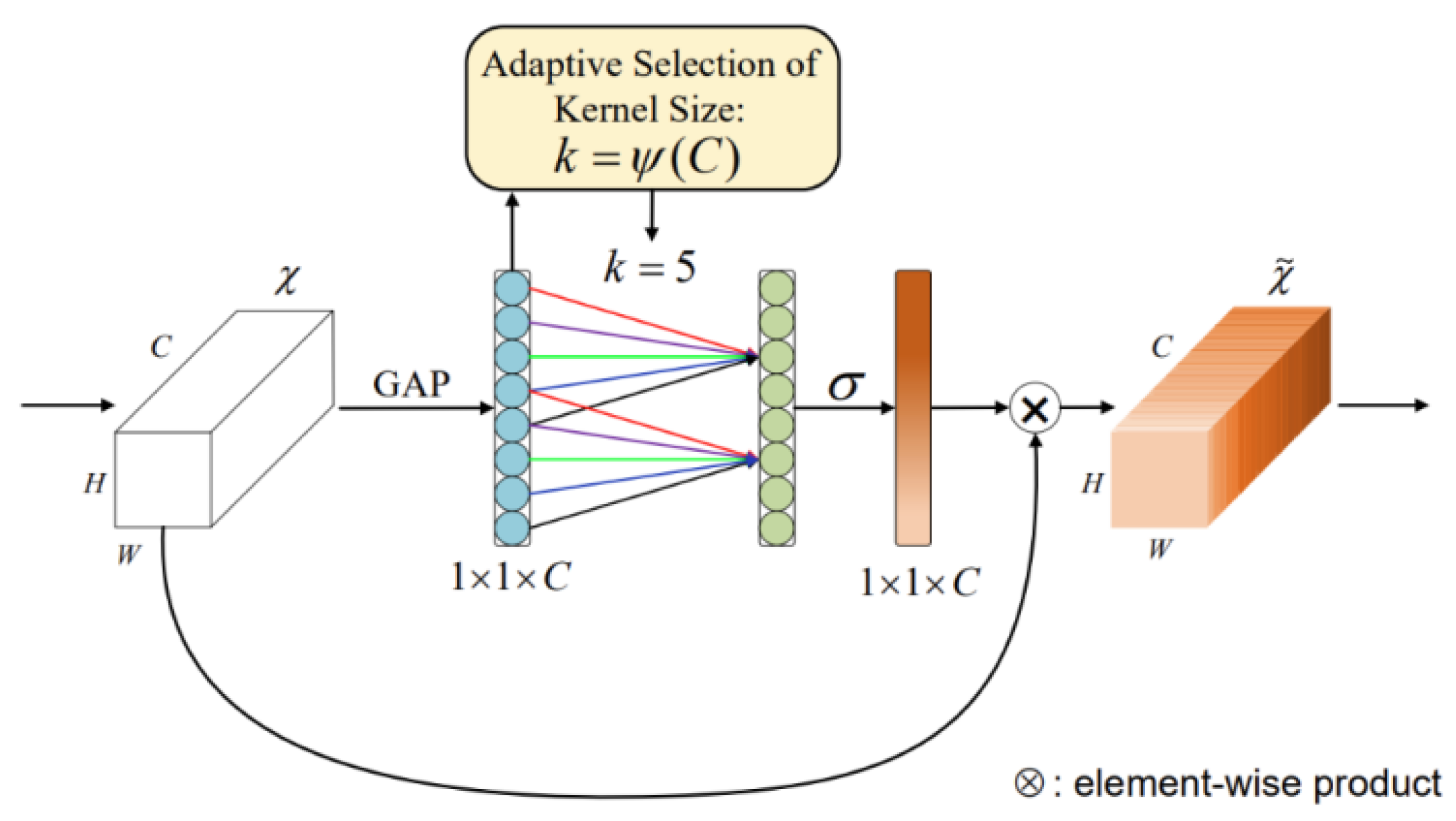
The ECA attention mechanism is a lightweight module, as shown in Figure 8. ECA attention is essentially a modified SE attention mechanism that proposes a no-dimensionality-reduction local cross-channel interaction strategy and an adaptive method for selecting one-dimensional convolution kernel size, thereby improving performance. Here are the detailed steps of the ECA attention mechanism:

Figure 8.
ECA module diagram.
- Global Average Pooling: Performs global average pooling operation on the input tensor, compressing the spatial dimension information of each channel into a scalar value.
- Dimension Adjustment: Adjusts the dimensions of the pooled tensor to prepare for subsequent convolution operations.
- Channel Convolution: Performs one-dimensional convolution operation on the adjusted tensor, with the convolution kernel sliding along the channel dimension. The formula for calculating the convolution kernel size in the ECA attention mechanism is as follows:where k represents the kernel size, c represents the number of channels, denotes logarithm with base 2, and and b represent hyperparameters, Here, can be set to 2, b can be set to 1, and denotes rounding to the nearest odd number.
- Activation Function: Apply the Sigmoid activation function to the convolved tensor to obtain attention weights for each channel.
- Weighted Output: Multiply these values with the corresponding elements of the original input features to obtain the final feature map.
As shown in Figure 8. The different colored lines (red, green, purple, blue, etc.) represent connections in the one-dimensional convolution operation, where the kernel size k is adaptively set to 5, as calculated using (19). These differently colored connections illustrate the channel interaction method, demonstrating how the ECA module achieves local cross-channel interaction without dimensionality reduction.
2.5. CCA-MSC Feature Enhancement Algorithm
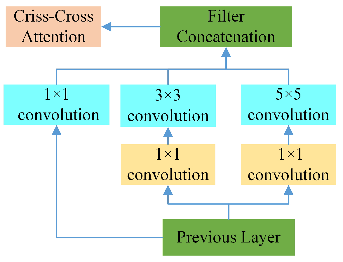
To enhance the network’s capability in capturing long-range dependencies, this research introduces a criss-cross attention (CCA) mechanism into the multi-scale convolutional feature extraction module (MSC), forming a novel CCA-MSC module. This innovative design aims to enhance feature representation capability, particularly in processing medium to long-range UAV acoustic signals.
The core concept of the CCA-MSC module is the application of criss-cross attention following the multi-scale feature extraction of the MSC module to capture long-range dependencies in feature maps. While the conventional MSC module extracts multi-scale features through parallel convolutions with varying kernel sizes, CCA effectively expands the receptive field by alternately computing attention in horizontal and vertical directions, enabling each position to acquire global contextual information. The structural diagram of this module is illustrated in Figure 9.
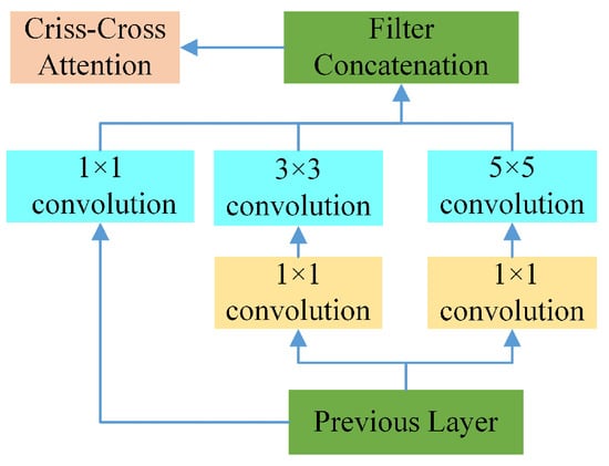
Figure 9.
CCA-MSC module.
2.5.1. Multi-Scale Convolution Feature Extraction Module (MSC)
Multi-scale convolution is a methodology in convolutional neural networks that extracts multi-scale features from input data through convolution kernels of varying sizes. This approach enables the capture of features with diverse dimensions and morphologies within the data, thereby enhancing model robustness and detection accuracy across heterogeneous inputs. It has found widespread applications in object detection, image segmentation, and classification tasks. The integration of features across multiple scales through multi-scale convolution facilitates richer feature representations. While this approach introduces additional computational complexity to the model architecture, it typically yields substantial performance improvements.
2.5.2. Attention Module CCA
Incorporating the CCA module into the network offers significant advantages. First, the CCA module effectively captures context information across the entire image, addressing the limitation of MSC’s primary reliance on local convolution operations. This introduction of global information is particularly crucial for tasks requiring comprehensive scene understanding. Second, CCA enhances feature representation capability at each pixel location through attention mechanisms while maintaining computational efficiency. Compared to fully connected attention mechanisms, CCA adopts a sparse connection approach, substantially reducing computational complexity. Overall, integrating the CCA module into the MSC module achieves an effective combination of local feature extraction and global context capture. While preserving the advantages of the original network structure, it significantly enhances its global information processing capabilities and feature representation abilities. This potentially improves performance across various classification tasks while maintaining computational efficiency and structural simplicity. The specific steps of the CCA module are outlined below:
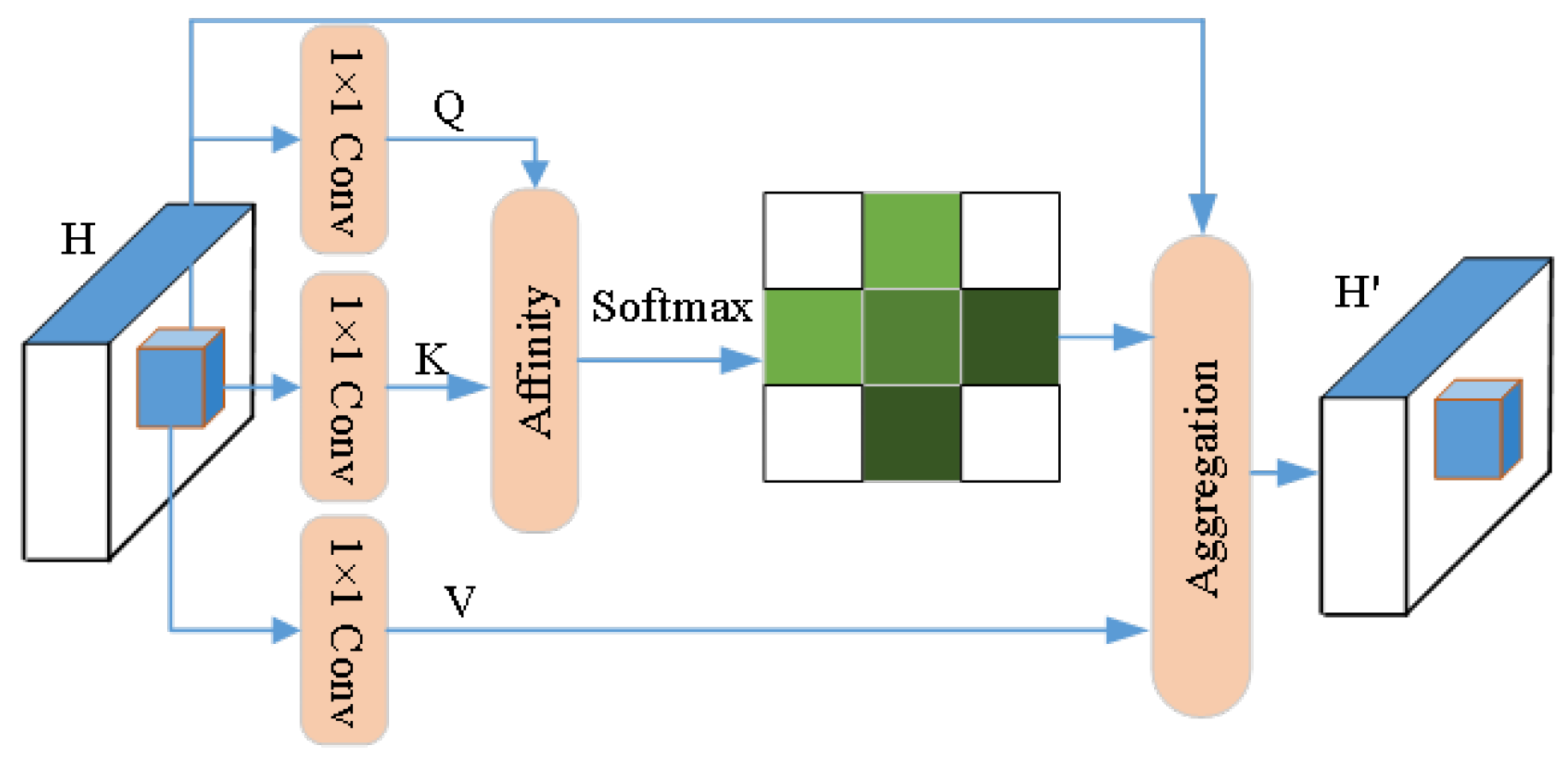
- Given an input feature map , the CCA module first applies 1 × 1 convolution to generate two feature maps Q and K, where . Here, represents the number of channels, typically smaller than C to reduce dimensionality. Subsequently, through the Affinity operation, an attention map is generated. For each point u in feature map Q, we extract its feature vector . Meanwhile, we collect a set of feature vectors from K, containing features at positions sharing the same row or column with u, where is the i-th element of . The Affinity operation is defined as:where represents the correlation between feature and . Subsequently, a softmax layer is applied to matrix D to compute the attention map.
- The feature projection is obtained by applying 1 × 1 convolution with the same number of channels to the feature mapping. As described above, for each feature point u in V’s spatial dimensions, we can obtain a vector . At the position corresponding to u, features are collected in both horizontal and vertical directions to form a collection . Through the aggregation operation to capture information, the attention matrix A is applied to the feature map V. The formula is defined as follows:where represents the scalar value of A at channel i and position u and denotes the feature vector in the output feature map. Figure 10 illustrates the schematic diagram of the CCA criss-cross attention mechanism.
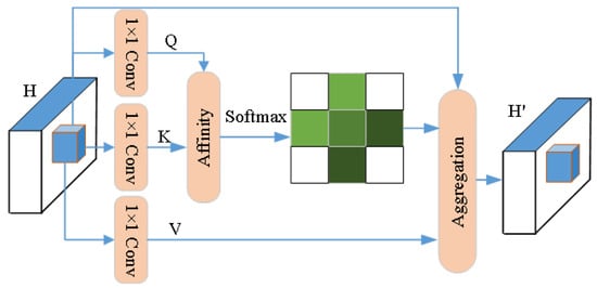 Figure 10. The CCA cross-attention mechanism.
3. Results and Discussion
3.1. Dataset Introduction
In this experiment, professional sound acquisition equipment was used to collect audio samples from four different types of drones at both short-range (0–10 m) and long-range (50 m) distances. The sampling frequency was set to 44,100 kHz with a single-channel configuration, and the recordings were segmented into 0.5-s audio clips. The short-range data were collected when the drones were flying within 0–10 m from the microphone, while the long-range (50 m) data were obtained when the drones were flying at the perimeter of a 50 m radius from the microphone. Subsequently, three main folders—training set, validation set, and test set—were created, with each containing four subfolders labeled “0”, “1”, “2”, and “3”, corresponding to the four drone types. The audio segments for each drone type were then distributed among these sets following a ratio, allocating 60% for training, 20% for validation, and 20% for testing. This methodology ensures a structured organization of the dataset while maintaining consistency and balance between the training and test sets. Table 1 presents the relevant dataset information for this experiment.

Table 1.
Dataset introduction.
This experiment employs a cross-distance noise recognition approach, where noise data collected at close range are used for training, while data collected at long range are used for testing. This cross-distance noise recognition method is used to verify whether the model has merely memorized the characteristic patterns of close-range signals or has truly learned the essential acoustic features of drones. If the model performs well on long-range data, it demonstrates strong recognition capabilities.
3.2. Experimental Environment and Indicators
Hardware Environment: CPU: Intel Core i9-13900HX, 16 GB RAM; Graphics card: NVIDIA RTX4060, 24 GB VRAM; Disk capacity: 1.2 TB.
Software Environment: Python: 3.7; TensorFlow: 1.15.
Operating System: Windows 11.
Evaluation Metrics: , , , and , which are defined as follows:
where , , , and represent True Positive, True Negative, False Positive, and False Negative, respectively. In multi-class classification problems, these metrics can be calculated in two ways:
- Macro-averaging: For each class, binary classification metrics are calculated separately (treating the current class as positive and all other classes as negative), and then the average is taken across all classes.
- Micro-averaging: The , , , and from all classes are accumulated, and then the overall metrics are calculated.
In our experiments, we adopted the macro-averaging method, which means we calculated the metrics for each class (four types of drones) separately and then took the average as the overall performance evaluation. This approach treats each class equally, regardless of class imbalance in the sample distribution.
3.3. Comparison of Experimental Results of Feature Fusion
This paper compares the proposed AF fusion algorithm with linear concatenation fusion algorithm and intermediate layer linear concatenation fusion algorithm through comparative experiments. The linear concatenation fusion algorithm operates at the feature level, with its core idea being the direct concatenation of different types of feature matrices along the feature dimension, forming a feature matrix with higher feature dimensions. This method preserves all information from the original features without introducing additional computational complexity. The middle layer feature map direct addition fusion method (Middle Fusion) is an acoustic feature fusion technique, which can be mathematically defined simply as directly adding MFCC and GFCC features after convolutional processing:
where and represent the initial acoustic features extracted by MFCC and GFCC, respectively, and denotes the convolution operation. In the specific implementation, we first apply identical parameterized convolution operations to both MFCC and GFCC acoustic features. Subsequently, we perform element-wise addition on these two processed feature maps to form the fused features, which are then fed into the subsequent network layers. Table 2 shows the results of the feature fusion experiments. Figure 11 present the confusion matrices for the three fusion algorithms.
Table 2.
Comparison results of three fusion methods.
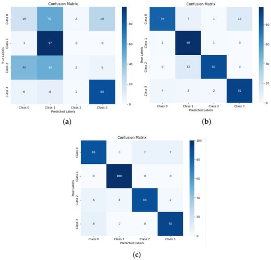
Figure 11.
Confusion matrices under three fusion methods: (a) the confusion matrix of the linear fusion method, (b) the confusion matrix of the middle fusion method, and (c) the confusion matrix of the AF fusion method.
This chapter compares three fusion methods: linear concatenation fusion, intermediate layer linear concatenation fusion, and AF module-based intermediate fusion. Among them, the AF-module-based fusion method demonstrates superior performance, achieving approximately 91.5% across metrics including recognition accuracy, precision, F1 score, and recall rate, significantly outperforming the other two methods. The advantage of the AF module lies in its innovative adaptive feature fusion mechanism, which effectively integrates MFCC and GFCC, two complementary acoustic features. Through its self-calibration mechanism, it dynamically adjusts the weights of different feature maps, highlighting important features while suppressing noise. This adaptive fusion approach not only enhances the discriminative ability of intermediate layer features but also fully utilizes the correlation and complementarity between feature maps, ultimately improving overall recognition performance.
3.4. Ablation Experiment
This paper systematically evaluates the impact of feature fusion methods and feature enhancement methods on UAV sound recognition performance through a series of ablation experiments. We first evaluated MFCC and GFCC as individual features to establish baseline performance. Subsequently, four key improvement steps were conducted:
- Intermediate Layer Feature Fusion: Simple fusion of MFCC and GFCC features at the network’s intermediate layer to explore the effectiveness of multi-feature combinations.
- AF Module Fusion: Introduction of the AF (Spatial and Channel Decorrelation Feature Fusion) module for more efficient intermediate layer feature fusion, forming the AF-MSC network architecture.
- Channel Attention Mechanism: Integration of channel attention (ECA) mechanism based on the AF module, constructing the AF-ECA-MSC architecture to further enhance the feature fusion algorithm’s effectiveness.
- (Criss-Cross Attention) Mechanism: While retaining the AF-ECA algorithm, introducing cross-channel attention (CCA) mechanism to the backbone network’s MSC module, ultimately forming the AF-ECA-CCA-MSC structure.
This series of experimental designs progressively optimized the feature fusion strategy and enhanced the fused features, progressing from single features to complex multi-feature fusion mechanisms and subsequent feature enhancement. Each step aimed to improve the model’s ability to recognize UAV sounds. Through this progressive improvement and systematic ablation experiments, the research clearly demonstrated the contribution of each innovative component in improving UAV sound recognition performance, validating the effectiveness and superiority of the proposed method. Table 3 presents the results of these ablation experiments.
Table 3.
Ablation study.
3.5. Comparative Experiments
The method proposed in this paper was compared with references [36,37] as well as three studies in the field of drone detection [38,39,40] for comparative experiments. The experimental results are shown in Table 4, using the dataset collected for this experiment. Reference [36] adopted a lightweight compact 1D-DCNN to reduce computational complexity and model the long-term dependency of speech emotion signals, using a fusion feature containing MFCC, RMS, zero-crossing rate, spectral centroid, spectral roll-off, LPCC, and other features. Reference [37] used a network called CNN-ATN for speaker emotion recognition, which adds an attention mechanism to the traditional convolutional neural network. The convolutional layer can effectively extract local features from speech signals, while the attention mechanism helps the network better focus on features important for emotion recognition. The paper extracts Mel-frequency cepstral coefficients (MFCCs) from audio to represent speech emotion information.
Table 4.
Comparative experiments on our collected dataset.
Reference [38] proposed a drone sound detection system based on feature result-level fusion, which uses Log-Mel spectrogram and Mel-frequency cepstral coefficients (MFCCs) to extract features from sound signals, inputs them separately into convolutional neural networks, and then fuses the results from the two networks using evidence theory to obtain the final detection result. This method achieved a detection accuracy of 94.5% within a range of 50 m, significantly outperforming traditional machine learning methods. Reference [39] proposed a machine-learning-inspired amateur drone sound detection method by extracting time-domain and frequency-domain features and using multilayer perceptron (MLP) and support vector machine (SVM) for classification. This method achieves 92% detection accuracy in noisy environments with low computational complexity, making it suitable for real-time application scenarios. Reference [40] developed an automated drone sound detection method based on skinny pattern analysis, which first uses wavelet transform to extract sound features, then employs skinny pattern analysis to capture the unique acoustic characteristics of drones, and finally performs detection through a random forest classifier. This method demonstrates high accuracy and robustness under various environmental conditions.
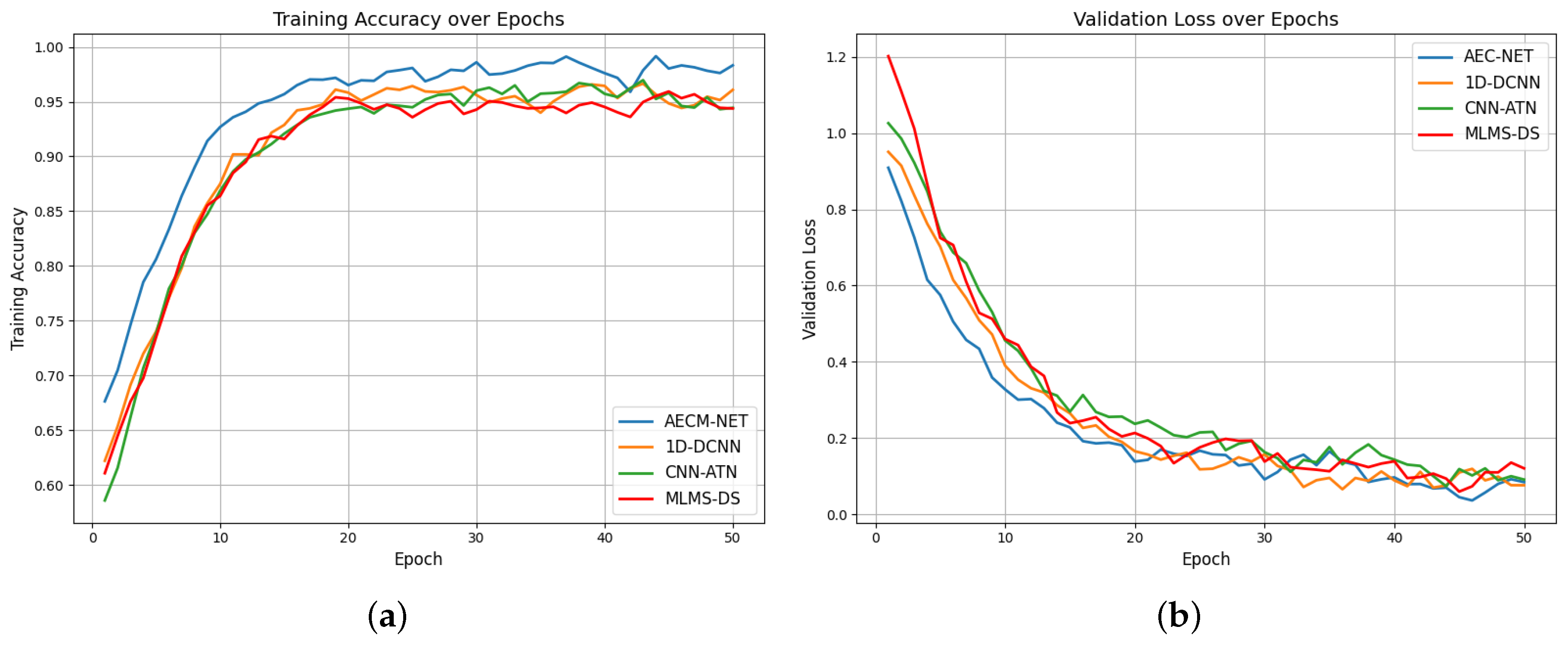
For the deep-learning-based methods, we further analyzed their performance changes during the training process, as shown in Figure 12. Since the ML-based method [39] using SVM and the Skinny pattern method [40] using random forest classifier are traditional machine learning techniques without epoch-based iterative training processes, Figure 12 only presents the training accuracy and validation loss curves for the four deep learning methods. From Figure 12a, it can be observed that our proposed ACEM-Net method consistently maintains higher accuracy throughout the training process and converges faster than the other two methods; Figure 12b shows that ACEM-Net’s validation loss decreases more rapidly and stabilizes better, indicating superior generalization capability.
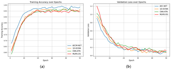
Figure 12.
The training and loss function curves of four network methods. Figure (a) shows the network training curves under four methods and Figure (b) shows the loss function curves.
As shown in Table 4, the proposed ACEM-Net method achieves the highest performance with 94.50% accuracy and an F1 score of 94.8%, outperforming all comparison methods. The CNN-ATN approach [37] ranks second with 92.60% accuracy, while the 1D-DCNN method [36] achieves 91.75% accuracy, despite utilizing multiple acoustic features. The three drone-specific detection methods [38,39,40] show relatively lower performance with accuracy rates between 89.50% and 90.80%. These results demonstrate that our ACEM-Net’s combination of MFCC and GFCC features with an efficient network architecture provides significant advantages (approximately 2–5% improvement) over existing approaches for drone sound detection tasks.
Cross-Dataset Validation
To further validate the robustness of our proposed ACEM-Net method, we conducted additional experiments using a publicly available drone sound dataset. For this cross-validation experiment, we utilized the drone audio dataset released by [41], which contains audio recordings of two commercial drone models: Bebop and Mambo, both manufactured by Parrot. This dataset is particularly valuable, as it includes both clean recordings and artificially augmented versions with various environmental noises, allowing for realistic testing scenarios.
The Al-Emadi dataset presents a challenging scenario, as it includes audio recordings from two distinct drone models with various background noise conditions. In their original work, Al-Emadi et al. [41] tested three deep learning approaches on this dataset for drone identification: CNN, RNN, and CRNN. Based on their comprehensive evaluation, they concluded that while CNN achieved the highest accuracy in their experiments, CRNN offered the most balanced performance considering both accuracy and computational efficiency, making it their recommended approach for practical applications.
As shown in Table 5, we implemented our ACEM-Net method on this same dataset and compared the results with the CRNN method from the original paper. Our ACEM-Net achieved 94.25% accuracy, outperforming the CRNN method by 2.03 percentage points. The precision, recall, and F1 scores of our method were also consistently higher, with improvements of 2.06%, 2.02%, and 2.17% respectively.
Table 5.
Performance comparison on the dataset of [41].
These results demonstrate that our ACEM-Net model maintains its performance advantage even when tested on an entirely different dataset with unique characteristics. The improved performance on the Al-Emadi dataset confirms the model’s strong generalization capabilities across different recording environments, drone types, and noise conditions. This cross-dataset validation provides compelling evidence for the robustness of our approach in real-world drone sound detection applications.
4. Conclusions
This paper proposes a novel network architecture, ACEM-Net, for high-precision recognition of UAV acoustic signals at medium to long distances. The innovations primarily focus on feature fusion and feature enhancement. In terms of feature fusion, the research utilizes MFCC and GFCC as complementary acoustic features and introduces an adaptive feature fusion (AF) module with a self-calibration mechanism. This module can dynamically adjust weights of different features, effectively highlighting important features while suppressing noise, demonstrating significant advantages over traditional linear concatenation and intermediate layer fusion methods.
For feature enhancement, the study incorporates an ECA channel attention mechanism after the AF module and embeds a CCA cross-attention mechanism in multi-scale feature extraction modules. This design not only captures long-range dependencies but also significantly enhances feature map representation capability. Additionally, the introduction of residual connections effectively addresses the gradient vanishing problem, further improving network performance.
To validate the method’s effectiveness, the research constructed a dataset containing audio samples from four types of UAVs at distances ranging from 0 to 50 m, using a cross-distance noise recognition approach for experimental validation. Through detailed ablation studies, the effectiveness of each innovative component was demonstrated. Comprehensive comparative experiments show that the proposed ACEM-Net achieves 94.50% accuracy and an F1 score of 94.8% on our collected dataset, significantly outperforming existing methods including 1D-DCNN (91.75%), CNN-ATN (92.60%), and other drone-specific detection approaches (with accuracy rates between 89.50% and 90.80%). The training process analysis further demonstrates that our method not only achieves higher overall accuracy but also converges faster with better stability compared to other deep learning approaches.
Moreover, cross-dataset validation on the publicly available Al-Emadi dataset confirms the robustness of our approach, with ACEM-Net achieving 94.25% accuracy and outperforming the CRNN method (92.22%) by approximately 2 percentage points across all metrics. This demonstrates the strong generalization capabilities of our model across different recording environments, drone types, and noise conditions.
This paper not only provides new theoretical insights into deep learning applications in acoustic signal processing but also makes important practical contributions to improving UAV recognition accuracy at medium to long distances and enhancing public safety. Future research directions include expanding the dataset to include more UAV types and environmental conditions, optimizing real-time performance, enhancing noise resistance capabilities, and integration with other sensing modalities. These advancements will further promote the development of acoustic-based UAV detection technologies.
Author Contributions
Conceptualization, X.L.; Methodology, J.R., Z.W. and J.Z.; Software, Z.W.; Validation, Z.W.; Formal analysis, J.R., Z.W. and J.Z.; Data curation, J.Z.; Writing—original draft, J.R.; Writing—review & editing, J.Z. and X.L.; Visualization, J.R.; Supervision, X.L.; Project administration, X.L. All authors have read and agreed to the published version of the manuscript.
Funding
This work was supported in part by the Science and Technology Plan Project of Yunnan Province Science and Technology Department (Grant No. 202301BD070001-194), in part by the National Natural Science Foundation of China (Grant Nos. 62363035 and 62201478), and in part by the Sichuan Science and Technology Program (Grant Nos. 2024NSFSC1434, 2024ZDZX0012).
Data Availability Statement
The code used in this study is publicly available on GitHub at https://github.com/wzjjjjjj/ECAM-NET-Code-and-UAV-datas/tree/main, accessed on 28 March 2025. The original contributions presented in this study are included in the article. The datasets used during the current study will be made available in the same GitHub repository in the future.
Conflicts of Interest
The authors declare no conflicts of interest.
References
- Radoglou–Grammatikis, P.; Sarigiannidis, P.; Lagkas, T.; Moscholios, I. A compilation of UAV applications for precision agriculture. Comput. Netw. 2020, 172, 107148. [Google Scholar]
- Liu, P.; Chen, A.Y.; Huang, Y.N.; Han, J.-Y.; Lai, J.-S.; Kang, S.-C.; Wu, T.-H.; Wen, M.-C.; Tsai, M.-H. A review of rotorcraft unmanned aerial vehicle (UAV) developments and applications in civil engineering. Smart Struct. Syst. 2014, 13, 1065–1094. [Google Scholar]
- Chávez, K. Learning on the fly: Drones in the Russian-Ukrainian war. Arms Control Today 2023, 53, 6–11. [Google Scholar]
- Fu, H.; Abeywickrama, S.; Zhang, L.; Yuen, C. Low-complexity portable passive drone surveillance via SDR-based signal processing. IEEE Commun. Mag. 2018, 56, 112–118. [Google Scholar]
- Jackman, A.; Hooper, L. Drone Incidents And misuse; University of Reading: Reading, UK, 2023. [Google Scholar]
- Guvenc, I.; Koohifar, F.; Singh, S.; Sichitiu, M.L.; Matolak, D. Detection, tracking, and interdiction for amateur drones. IEEE Commun. Mag. 2018, 56, 75–81. [Google Scholar]
- Yan, J.; Hu, H.; Gong, J.; Kong, D.; Li, D. Exploring Radar Micro-Doppler Signatures for Recognition of Drone Types. Drones 2023, 7, 280. [Google Scholar] [CrossRef]
- Lee, D.; La, W.G.; Kim, H. Drone detection and identification system using artificial intelligence. In Proceedings of the 2018 International Conference on Information and Communication Technology Convergence (ICTC), Jeju, Republic of Korea, 17–19 October 2018; IEEE: New York, NY, USA, 2018; pp. 1131–1133. [Google Scholar]
- Aouladhadj, D.; Kpre, E.; Deniau, V.; Kharchouf, A.; Gransart, C.; Gaquiere, C. Drone Detection and Tracking Using RF Identification Signals. Sensors 2023, 23, 7650. [Google Scholar] [CrossRef]
- Kolamunna, H.; Dahanayaka, T.; Li, J.; Seneviratne, S.; Thilakaratne, K.; Zomaya, A.Y.; Seneviratne, A. Droneprint: Acoustic signatures for open-set drone detection and identification with online data. Proc. ACM Interact. Mob. Wearable Ubiquitous Technol. 2021, 5, 1–31. [Google Scholar]
- Cerutti, G.; Prasad, R.; Brutti, A.; Farella, E. Compact recurrent neural networks for acoustic event detection on low-energy low-complexity platforms. IEEE J. Sel. Top. Signal Process. 2020, 14, 654–664. [Google Scholar]
- Kong, Q.; Xu, Y.; Sobieraj, I.; Wang, W.; Plumbley, M.D. Sound event detection and time-frequency segmentation from weakly labelled data. IEEE-ACM Trans. Audio Speech Lang. 2019, 27, 777–787. [Google Scholar]
- Solera-Ureña, R.; Padrell-Sendra, J.; Martín-Iglesias, D.; Gallardo-Antolín, A.; Peláez-Moreno, C.; Díaz-de-María, F. SVMs for automatic speech recognition: A survey. In Progress in Nonlinear Speech Processing; Springer: Berlin/Heidelberg, Germany, 2007; pp. 190–216. [Google Scholar]
- Kumar, G.S.; Raju, K.A.P.; Cpvnj, M.R.; Satheesh, P. Speaker recognition using GMM. Int. J. Eng. Sci. Technol. 2010, 2, 2428–2436. [Google Scholar]
- Jarng, S.S. HMM voice recognition algorithm coding. In Proceedings of the 2011 International Conference on Information Science and Applications, Jeju, Republic of Korea, 26–29 April 2011; IEEE: New York, NY, USA, 2011; pp. 1–7. [Google Scholar]
- Mohanapriya, S.P.; Sumesh, E.P.; Karthika, R. Environmental sound recognition using Gaussian mixture model and neural network classifier. In Proceedings of the 2014 International Conference on Green Computing Communication and Electrical Engineering (ICGCCEE), Coimbatore, India, 6–8 March 2014; IEEE: New York, NY, USA, 2014; pp. 1–5. [Google Scholar]
- Palaniappan, R.; Sundaraj, K. Respiratory sound classification using cepstral features and support vector machine. In Proceedings of the 2013 IEEE Recent Advances in Intelligent Computational Systems (RAICS), Thiruvananthapuram, India, 3–5 December 2020; IEEE: New York, NY, USA, 2013; pp. 132–136. [Google Scholar]
- Chauhan, S.; Wang, P.; Lim, C.S.; Anantharaman, V. A computer-aided MFCC-based HMM system for automatic auscultation. Comput. Biol. Med. 2008, 38, 221–233. [Google Scholar] [PubMed]
- Wang, Y.; Sun, B.; Yang, X.; Meng, Q. Heart sound identification based on MFCC and short-term energy. In Proceedings of the 2017 Chinese Automation Congress (CAC), Jinan, China, 20–22 October 2017; IEEE: New York, NY, USA, 2017; pp. 7411–7415. [Google Scholar]
- Hanifa, R.M.; Isa, K.; Mohamad, S.; Shah, S.M.; Nathan, S.S.; Ramle, R.; Berahim, M. Voiced and unvoiced separation in Malay speech using zero crossing rate and energy. Indones. J. Electr. Eng. Comput. Sci. 2019, 16, 775–780. [Google Scholar]
- Hinton, G.E.; Osindero, S.; Teh, Y.W. A fast learning algorithm for deep belief nets. Neural Comput. 2006, 18, 1527–1554. [Google Scholar]
- Bae, H.S.; Lee, H.J.; Lee, S.G. Voice recognition based on adaptive MFCC and deep learning. In Proceedings of the 2016 IEEE 11th Conference on Industrial Electronics and Applications (ICIEA), Hefei, China, 5–7 June 2016; IEEE: New York, NY, USA, 2016; pp. 1542–1546. [Google Scholar]
- Katta, S.S.; Nandyala, S.; Viegas, E.K.; Agrawal, N.; Fitwi, A.; Detweiler, C.; Ly, N.T.; Mohanty, S.P. Benchmarking audio-based deep learning models for detection and identification of unmanned aerial vehicles. In Proceedings of the 2022 Workshop on Benchmarking Cyber-Physical Systems and Internet of Things (CPS-IoTBench), Pittsburgh, PA, USA, 17 May 2022; IEEE: New York, NY, USA, 2022; pp. 7–11. [Google Scholar]
- Solis, E.R.; Shashev, D.V.; Shidlovskiy, S.V. Implementation of audio recognition system for unmanned aerial vehicles. In Proceedings of the 2021 International Siberian Conference on Control and Communications (SIBCON), Kazan, Russia, 13–15 May 2021; IEEE: New York, NY, USA, 2021; pp. 1–8. [Google Scholar]
- Geng, Q.S.; Wang, F.H.; Zhou, D.X. Mechanical fault diagnosis of power transformer by GFCC time-frequency map of acoustic signal and convolutional neural network. In Proceedings of the 2019 IEEE Sustainable Power and Energy Conference (iSPEC), Beijing, China, 21–23 November 2019; IEEE: New York, NY, USA, 2019; pp. 2106–2110. [Google Scholar]
- Seo, Y.; Jang, B.; Im, S. Drone detection using convolutional neural networks with acoustic STFT features. In Proceedings of the 2018 15th IEEE International Conference on Advanced Video and Signal Based Surveillance (AVSS), Auckland, New Zealand, 27–30 November 2018; IEEE: New York, NY, USA, 2018; pp. 1–6. [Google Scholar]
- Yan, N.; Chen, A.; Zhou, G.; Zhang, Z.; Liu, X.; Wang, J.; Liu, Z.; Chen, W. Birdsong classification based on multi-feature fusion. Multimed. Tools Appl. 2021, 80, 36529–36547. [Google Scholar]
- Jahangir, R.; Teh, Y.W.; Memon, N.A.; Mujtaba, G.; Zareei, M.; Ishtiaq, U.; Akhtar, M.Z.; Ali, I. Text-independent speaker identification through feature fusion and deep neural network. IEEE Access 2020, 8, 32187–32202. [Google Scholar]
- Dalila, C.; Saddek, B.; Amine, N.A. Feature level fusion of face and voice biometrics systems using artificial neural network for personal recognition. Informatica 2020, 44, 1. [Google Scholar]
- Hu, S.P.; Chu, Y.H.; Tang, L.; Zhou, G.X.; Chen, A.B.; Sun, Y.R. A lightweight multi-sensory field-based dual-feature fusion residual network for bird song recognition. Appl. Soft Comput. 2023, 146, 17. [Google Scholar]
- Chen, L.; Liu, L. SE-TDN-LSTM speaker recognition algorithm based on residual connection. In Proceedings of the 2024 5th International Conference on Computer Engineering and Application (ICCEA), Hangzhou, China, 12–14 April 2024; IEEE: New York, NY, USA, 2024; pp. 1324–1328. [Google Scholar]
- Zhang, J.; Wei, X.; Wang, Z. The Recognition Algorithm of Two-Phase Flow Patterns Based on GoogLeNet+ 5 Coord Attention. Micromachines 2023, 14, 462. [Google Scholar]
- Huang, Z.; Wang, X.; Huang, L.; Huang, C.; Wei, Y.; Liu, W. CCNet: Criss-cross attention for semantic segmentation. In Proceedings of the IEEE/CVF International Conference on Computer Vision, Seoul, Republic of Korea, 27 October–2 November 2019; pp. 603–612. [Google Scholar]
- Shi, L.; Ahmad, I.; He, Y.J.; Chang, K. Hidden Markov model based drone sound recognition using MFCC technique in practical noisy environments. J. Commun. Netw. 2018, 20, 509–518. [Google Scholar]
- Xue, S.; Li, G.; Lü, Q.; Mao, Y. Sound recognition method of an anti-UAV system based on a convolutional neural network. Chin. J. Eng. 2020, 42, 1516–1524. [Google Scholar]
- Bhangale, K.; Kothandaraman, M. Speech emotion recognition based on multiple acoustic features and deep convolutional neural network. Electronics 2023, 12, 839. [Google Scholar] [CrossRef]
- Mountzouris, K.; Perikos, I.; Hatzilygeroudis, I. Speech Emotion Recognition Using Convolutional Neural Networks with Attention Mechanism. Electronics 2023, 12, 4376. [Google Scholar] [CrossRef]
- Dong, Q.; Liu, Y.; Liu, X. Drone sound detection system based on feature result-level fusion using deep learning. Multimed. Tools Appl. 2023, 82, 149–171. [Google Scholar]
- Anwar, M.Z.; Kaleem, Z.; Jamalipour, A. Machine learning inspired sound-based amateur drone detection for public safety applications. IEEE Trans. Veh. Technol. 2019, 68, 2526–2534. [Google Scholar]
- Akbal, E.; Akbal, A.; Dogan, S.; Cakmak, F.; Toth, B.; Akyildiz, I.F. An automated accurate sound-based amateur drone detection method based on skinny pattern. Digit. Signal Process. 2023, 136, 104012. [Google Scholar]
- Al-Emadi, S.; Al-Ali, A.; Mohammad, A.; Al-Ali, A. Audio based drone detection and identification using deep learning. In Proceedings of the 2019 15th International Wireless Communications & Mobile Computing Conference (IWCMC), Tangier, Morocco, 24–28 June 2019; IEEE: New York, NY, USA, 2019; pp. 459–464. [Google Scholar]


Disclaimer/Publisher’s Note: The statements, opinions and data contained in all publications are solely those of the individual author(s) and contributor(s) and not of MDPI and/or the editor(s). MDPI and/or the editor(s) disclaim responsibility for any injury to people or property resulting from any ideas, methods, instructions or products referred to in the content. |
© 2025 by the authors. Licensee MDPI, Basel, Switzerland. This article is an open access article distributed under the terms and conditions of the Creative Commons Attribution (CC BY) license (https://creativecommons.org/licenses/by/4.0/).