Optimal Innovation-Based Deception Attacks on Multi-Channel Cyber–Physical Systems

Abstract

This article addresses the optimal scheduling problem for linear deception attacks in multi-channel cyber–physical systems. The scenario where the attacker can only attack part of the channels due to energy constraints is considered. The effectiveness and stealthiness of attacks are quantified using state estimation error and Kullback–Leibler divergence, respectively. Unlike existing strategies relying on zero-mean Gaussian distributions, we propose a generalized attack model with Gaussian distributions characterized by time-varying means. Based on this model, an optimal stealthy attack strategy is designed to maximize remote estimation error while ensuring stealthiness. By analyzing correlations among variables in the objective function, the solution is decomposed into a semi-definite programming problem and a 0–1 programming problem. This approach yields the modified innovation and an attack scheduling matrix. Finally, numerical simulations validate the theoretical results.

1. Introduction

Cyber–physical systems (CPSs) seamlessly merge computational processes with physical components via real-time networked communication, thereby achieving coordinated collection, processing, and exchange of information [1]. These systems have demonstrated broad applicability across diverse domains [2,3], including vehicle platooning [4], smart grid management [5], and healthcare systems [6]. However, cyberattacks targeting communication channels can destabilize CPSs by compromising their operational integrity. Notable cybersecurity incidents, such as the Stuxnet virus [7] and the Maroochy water services breach [8], further highlight these vulnerabilities. Consequently, the security of CPSs has become a critical research focus.

Attack detection schemes are predominantly categorized into knowledge-driven and data-driven methodologies [9]. Among knowledge-driven systems, residual-based statistical methods stand out as one of the most representative detection strategies. Common implementations include the Chi-square (${\chi }^2$) detector, Euclidean detector, Kullback–Leibler divergence (KLD) detector and so on. The core principle involves generating a residual sequence by comparing sensor measurements with system estimations, followed by evaluating this residual against predefined thresholds to identify potential attacks. For data-driven approaches, machine learning (ML) and deep learning (DL) techniques are employed to model behavioral patterns in CPS. Attacks are flagged when significant deviations arise between observed data and model-predicted associations. ML algorithms, such as support vector machines (SVM), logistic regression, naïve Bayes, K-means clustering, and decision trees, utilize training data to achieve sophisticated pattern-matching capabilities. Notably, Aldallal et al. proposed a hybrid intrusion detection model that synergistically integrates the classification precision of the SVM with the global optimization capability of the genetic algorithm (GA) [10]. By employing a novel fitness function to optimize accuracy evaluation in cloud computing environments, this methodology not only addresses cloud attack detection challenges but also maintains adaptability to evolving dynamic threats.

Existing research mainly categorizes cyberattacks into two classes: denial-of-service (DoS) and deception attacks. Network communication is blocked in DoS attacks, thereby preventing sensors or actuators from obtaining valid data [11,12]. However, if defensive mechanisms reject transmitted data packets, the attack can be readily detected, thereby minimizing its impact on system performance [13,14,15]. Deception attacks are intentionally crafted by adversaries to intercept and modify in-transit data while maintaining stealthiness, thereby degrading system performance. A seminal study on power grid state estimation first introduced the concept of false data injection (FDI) attacks [16]. Attackers can arbitrarily manipulate state estimation results through two strategies: restricting access to measurement devices or exploiting resource constraints to compromise them. To evade detection by the ${\chi }^2$ detector, Guo et al. developed a strictly stealthy attack that preserves identical statistical characteristics before and after the attack [17]. Based on this, Ren et al. proposed an enhanced strictly stealthy attack strategy that incorporates all available historical innovation data [18]. However, deception attacks against ${\chi }^2$ detectors constitute a class of highly stealth attacks. Such attacks can be effectively identified through KLD detectors with properly configured thresholds. Yang et al. devised a fully stealthy attack strategy for CPSs with KLD detectors, eliminating the impact of attacks on innovation [19]. Recent studies have widely adopted KLD as a metric to quantify attack stealthiness in CPSs across diverse detector architectures. An $ϵ$-stealth attack strategy balancing a fixed stealthiness level and maximizing estimating performance loss was developed in [20]. A novel linear attack strategy grounded in innovation was proposed in [21], where the KLD between the original innovation and the modified innovation was employed as a measure of attack stealthiness. The attack strategy sacrifices certain stealth in exchange for improved attack performance. Different from the linear attack strategy that required a zero-mean Gaussian distribution [21], an attack scheme based on the innovation of time-invariant mean Gaussian distribution was proposed in [22].

While the aforementioned studies predominantly address deception attacks in single communication channels, the security of multi-channel systems has emerged as a critical research focus. In [23], a game-theoretic framework was employed to analyze resource allocation strategies for defenders and deception attackers in multi-channel systems. In [24], optimal deception attacks were proposed for systems equipped with ${\chi }^2$ detectors. These attack strategies utilized KLD as a stealthiness metric and were designed to meet both strict and relaxed stealthiness criteria. In [25,26], multi-channel systems with fixed attack locations across different time steps were considered, a limitation that significantly reduced the practicality of the proposed strategies. Recently, in [27], under the constraint that the KLD value did not exceed the preset threshold, the real energy constraint of the attacker was considered, which limited the attacker to targeting only some of the channels at each time step. In this way, the switching location attack strategy was optimized. In [28], innovations from different channels were linearly combined to derive the remote estimation error. Multi-channel attacks are inherently more complex than their single-channel counterparts, as attack parameters and scheduling variables need to be carefully balanced to maximize remote estimation error. However, these attack strategies have two limitations: (1) The attack model follows a Gaussian distribution with a fixed mean. (2) The objective function focuses on maximizing the estimation error at a specific time step.

Inspired by this, a linear deception attack model based on a Gaussian distribution with a time-varying mean is established, and the optimal attack scheduling under the attacker’s energy constraints is investigated, with KLD utilized as an indicator of attack stealth. To effectively degrade the estimation effect of the system, the optimal stealthy attack scheme is required to maximize the cumulative estimation error during the attack period while maintaining the stealthiness of the attack. The primary contributions of this study are summarized as follows:

• This paper introduces the cumulative estimation error over a finite time horizon as a metric to quantify the impact of attacks on the estimation performance degradation of multi-channel CPSs. This method is more complex and more reasonable, as it accounts for the remote estimation error over the entire attack duration rather than at a specific time point.
• An attack model based on the Gaussian distribution with a time-varying mean is proposed. Based on this model, the optimal attack strategy for multi-channel systems is investigated. This approach is more general and more complicated as it introduces more decision variables.
• The time-varying covariance of the modified innovation results in a significant increase in estimation error. An algorithm for generating optimal stealthy attacks is proposed, enabling offline calculation of attack scheduling to alleviate the pressure of online calculation.

The rest of the article is constructed as follows. Section 2 reviews the related work in this area. Section 3 considers the system structure and the modeling of the research problem. The key findings and the proposed attack scheme are presented in Section 4. Section 5 simulates relevant theorems. Finally, the paper is summarized in Section 6.

2. Related Work

In this section, we provide a concise summary of recent advances in innovation-based deception attack strategies, including their current research status and application scenarios.

2.1. Research Status

In the previous work [21], the innovation-driven attack model under single-channel CPS was explored to maximize the system estimation error at each moment. In  [22], a Gaussian attack strategy with time-invariant mean was proposed to maximize the cumulative estimation error over finite-time horizons. On this basis, in [27,28], the architecture was extended to multi-channel CPSs, and the attack strategies were investigated to maximize the terminal estimation error under energy constraint. A critical limitation arises from the proposed attack strategies’ lack of generality, stemming from their fundamental reliance on constant-mean Gaussian distribution assumptions. Since the attacker has knowledge of the attack’s start and end times, it is reasonable that the objective shifts from maximizing the estimation error at specific time steps to maximizing the cumulative estimation error throughout the attack duration. Nevertheless, the formulation of optimal attack scheduling under this objective has not been addressed in the existing literature. A comprehensive synopsis of the comparison among related works is presented in

Table 1. Comparative analysis of related research metrics.

Related Works	Channel Type	Objective	Mean	Covariance
This Paper	Multi-Channel	Maximize the Cumulative Estimation Error	Time-Varying	Time-Varying
Guo et al. [21]	Single-Channel	Maximize the Estimation Error at Each Moment	Zero	Time-Invariant
Li et al. [27,28]	Multi-Channel	Maximize the Terminal Estimation Error	Zero	Time-Varying
Li et al. [22]	Single-Channel	Maximize the Cumulative Estimation Error	Time-Invariant	Time-Invariant

.

2.2. Application Scenarios

To enhance the applicability of the attack strategy, discussions are provided for several classic CPS scenarios:

• Smart Grid: The proposed optimal attack scheduling can degrade state estimation accuracy by disrupting multi-channel measurement consistency. For wide-area measurement systems (WAMS) with high-frequency sampling, the attack strategy requires further optimization of temporal window parameters to evade dynamic residual-based detection mechanisms.
• SCADA Systems: The periodic data transmission characteristics of protocols (e.g., Modbus, DNP3) necessitate synchronization between attack scheduling and data update cycles. While the energy constraint model aligns with resource limitations of attackers in industrial control systems (ICS), additional considerations must address the latency sensitivity of real-time control loops.
• Vehicle-to-Everything (V2X) Networks: The strategy can extend to multi-vehicle cooperative attack scenarios. By switching attack channels among different vehicles, it disrupts collaborative perception algorithms in traffic flow while leveraging the time-varying mean model to bypass location-correlation-based detection.

This analysis demonstrates the adaptability of the framework across CPS architectures, with scenario-specific parameter tuning ensuring compatibility with domain-specific communication protocols and defense mechanisms.

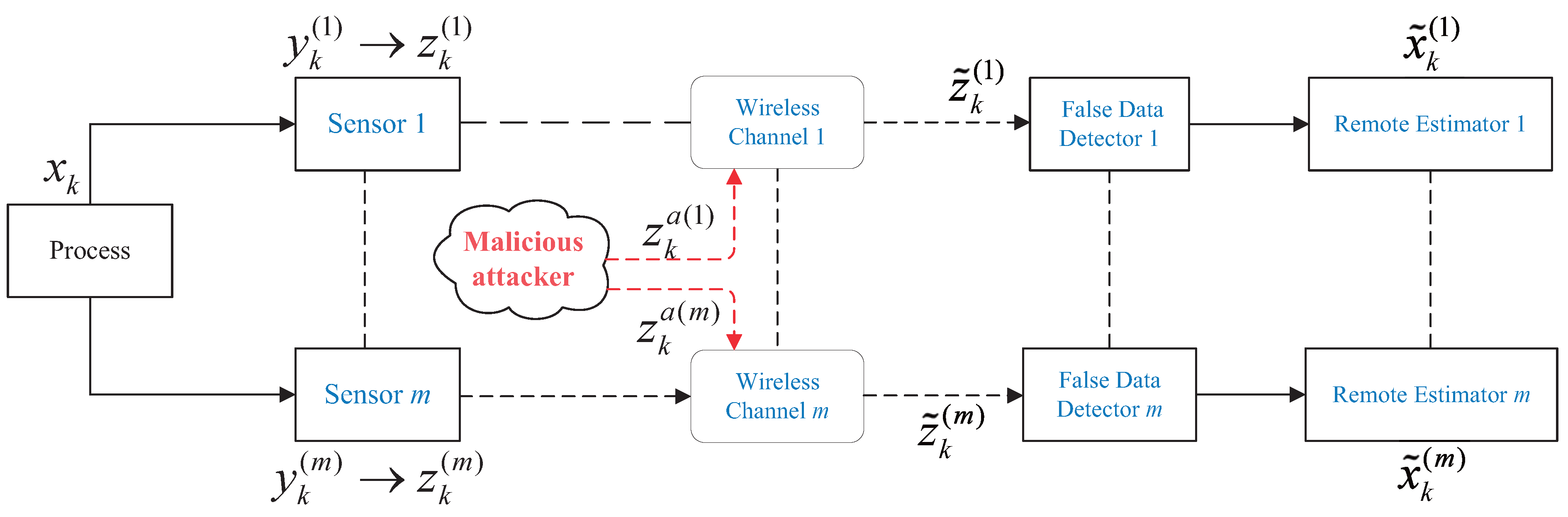
3. System Framework and Problem Formulation

This paper studies a CPS with m channels, as illustrated in Figure 1. Each sensor is capable of measuring the state of the relevant process and calculating the corresponding innovation, which is then transmitted to the remote estimator via the associated wireless communication channel. The attackers attempt to intercept and forge transmitted innovation signals, deliberately inducing deviations in state estimation while maintaining stealth characteristics against anomaly detectors. The detailed design of each physical component will be described in the following text.

3.1. Process Model

$\mathbb{H}=\{1,2,...,m\}$ is used to represent the index set of sensors. A linear discrete-time process is considered, and the specific model is described as

$$x_{k+1}=A{x}_k+w_k,$$

(1)

$$y_k^{\left(i\right)}=C^{\left(i\right)}{x}_k+v_k^{\left(i\right)},$$

(2)

where $i\in \mathbb{H}$, $k\in \mathbb{N}$ is the time step index. $x_k\in {\mathbb{R}}^l$ signifies the state of the process at time k. $y_k^{\left(i\right)}\in {\mathbb{R}}^{n_i}$ shows the measurement of sensor i at time k. $A\in {\mathbb{R}}^{l\times l}$ and $C^{\left(i\right)}\in {\mathbb{R}}^{n_i\times l}$ are the system matrix and measurement matrix, respectively. $w_k$ and $v_k^{\left(i\right)}$ are Gaussian noises with covariances $Q\ge 0$ and $R^{\left(i\right)}\ge 0$, respectively. For any time k, the initial state $x_0$ satisfies $x_0\sim \mathcal{N}(0,{\Pi }_0)$, and is independent of $w_k$ and $v_k^{\left(i\right)}$.

3.2. State Estimator

The local sensor first transforms the measurement data into an innovation and then transmits it to the remote estimator via the wireless channel. The remote estimators employ Kalman filters (KFs) to estimate the system state by

$${\widehat{x}}_k^{\left(i\right)-}=A{\widehat{x}}_{k-1}^{\left(i\right)},$$

(3)

$$P_k^{\left(i\right)-}=A{P}_{k-1}^{\left(i\right)}{A}^T+Q,$$

(4)

$$G_k^{\left(i\right)}=P_k^{\left(i\right)-}{C}^{\left(i\right)T}{\left(C^{\left(i\right)}{P}_k^{\left(i\right)-}{C}^{\left(i\right)T}+R^{\left(i\right)}\right)}^{-1},$$

(5)

$${\widehat{x}}_k^{\left(i\right)}={\widehat{x}}_k^{\left(i\right)-}+G_k^{\left(i\right)}\left(y_k^{\left(i\right)}-C^{\left(i\right)}{\widehat{x}}_k^{\left(i\right)-}\right),$$

(6)

$$P_k^{\left(i\right)}=\left(I-G_k^{\left(i\right)}{C}^{\left(i\right)}\right)P_k^{\left(i\right)-},$$

(7)

where ${\widehat{x}}_k^{\left(i\right)-}$ and ${\widehat{x}}_k^{\left(i\right)}$ are the priori and posteriori minimum mean square error (MMSE) estimates of state $x_k$ given by the remote estimator, respectively. $P_k^{\left(i\right)-}$ and $P_k^{\left(i\right)}$ are relevant error covariances, which are expressed as follows:

$$P_k^{\left(i\right)-}\triangleq \mathbb{E}\left[\left(x_k-{\widehat{x}}_k^{\left(i\right)-}\right){\left(x_k-{\widehat{x}}_k^{\left(i\right)-}\right)}^T\right],$$

(8)

$$P_k^{\left(i\right)}\triangleq \mathbb{E}\left[\left(x_k-{\widehat{x}}_k^{\left(i\right)}\right){\left(x_k-{\widehat{x}}_k^{\left(i\right)}\right)}^T\right].$$

(9)

The iteration starts from ${\widehat{x}}_0^{\left(i\right)-}$ = 0 and $P_0^{\left(i\right)-}={\Pi }_0$. Under the premise that the pair $(A,C^{\left(i\right)})$ is detectable and $(A,\sqrt{Q})$ is stabilizable, the KF will be asymptotically stable for any initial error covariance [29]. The error covariance of the steady state is expressed as ${\overline{P}}^{\left(i\right)}\triangleq \underset{k\to \infty }{lim}{P}_k^{\left(i\right)-}$ and the fixed gain is ${\overline{G}}^{\left(i\right)}\triangleq {\overline{P}}^{\left(i\right)}{C}^{\left(i\right)T}{{\Sigma }^{\left(i\right)}}^{-1}$. The local innovation $z_k^{\left(i\right)}$ is a zero-mean i.i.d. Gaussian variable with covariance ${\Sigma }^{\left(i\right)}=(C^{\left(i\right)}{\overline{P}}^{\left(i\right)}{C}^{\left(i\right)T}+R^{\left(i\right)})$, calculated by the sensor i from $z_k^{\left(i\right)}=y_k^{\left(i\right)}-C^{\left(i\right)}{\widehat{x}}_k^{\left(i\right)-}$.

Remark 1.

Compared with traditional sensors [30], intelligent sensors enhance computational precision and enable efficient transmission. The decision to transmit the innovation $z_k^{\left(i\right)}$ to the remote estimator, instead of ${\widehat{x}}_k^{\left(i\right)}$ or $y_k^{\left(i\right)}$, stems from the more stable statistical properties of $z_k^{\left(i\right)}$. This stability facilitates the detector’s ability to identify whether an attack has modified the innovation.

3.3. Detector and Stealthiness Condition

A detector is needed at the remote end to detect network attacks by checking the statistical properties of the transmitted innovation. We assume that using the well-known ${\chi }^2$ detector as the false data detector. This detector evaluates the statistical properties of the innovation sequence via the following function:

$$h\left(z_k^{\left(i\right)}\right)=z_k^{\left(i\right)T}{\Sigma }^{{\left(i\right)}^{-1}}{z}_k^{\left(i\right)},$$

(10)

where ${\Sigma }^{\left(i\right)}$ denotes the covariance matrix of the innovation $z_k^{\left(i\right)}$, and $h\left(z_k^{\left(i\right)}\right)$ follows the ${\chi }^2$ distribution with $n_i$ degrees of freedom. The alarm will be triggered if the statistic exceeds a predefined threshold.

Similar to the stealth evaluation criteria established in [31,32], the KLD between the original sequence and the modified sequence is used as the core stealth metric to strictly quantify the stealth characteristics of the attack. For two Gaussian-distributed variables, the KLD is defined as follows.

Definition 1

(KLD). The KLD quantifies the discrepancy between two probability distributions. Let α and β be characterized by their probability density functions $f_{\alpha }$ and $f_{\beta }$, respectively. The KLD from α to β is formally defined as

$$D(\alpha \parallel \beta )={\int }_{-\infty }^{+\infty }log{\displaystyle \frac{f_{\alpha }\left(\gamma \right)}{f_{\beta }\left(\gamma \right)}}{f}_{\alpha }\left(\gamma \right)d\gamma .$$

(11)

In particular, if $\alpha$ and $\beta$ are n-dimensional Gaussian random variables distributed as $\alpha \sim \mathcal{N}({\mu }_{\alpha },{\Sigma }_{\alpha })$ and $\beta \sim \mathcal{N}({\mu }_{\beta },{\Sigma }_{\beta })$, respectively, (11) reduces to

$$\begin{array}{cc}\hfill D(\alpha \parallel \beta )=& {\displaystyle \frac{1}{2}}(log{\displaystyle \frac{|{\Sigma }_{\beta }|}{|{\Sigma }_{\alpha }|}}-n+\mathrm{Tr}\left({\Sigma }_{\beta }^{-1}{\Sigma }_{\alpha }\right)+{\left({\mu }_{\beta }-{\mu }_{\alpha }\right)}^T\hfill \\ \hfill & {\Sigma }_{\beta }^{-1}\left({\mu }_{\beta }-{\mu }_{\alpha }\right)).\hfill \end{array}$$

(12)

A smaller difference between the two distributions results in a lower KLD value. Notably, $D(\alpha \Vert \beta )=0$ if $f_{\alpha }=f_{\beta }$.

Definition 2

(Stealthiness Condition). For an arbitrary channel i, the attacker must ensure statistical similarity between the modified and original innovations to avoid triggering the detector’s alarm. Therefore, the stealthiness condition for the attack is given by

$$D({\tilde{z}}_k^{\left(i\right)}\parallel z_k^{\left(i\right)})⩽\delta ,$$

(13)

where ${\tilde{z}}_k^{\left(i\right)}$ is the innovation collected on the remote end, and δ is the threshold.

Remark 2.

Since the threshold satisfies $\delta >0$, the attack is not strictly stealthy [20,21]. In this circumstance, stealthiness has to be compromised to tolerate a larger estimation error. Subsequently, the condition for strict stealthiness was thoroughly investigated in  [19].

3.4. Energy Restriction

Definition 3.

Unlike attackers considered in [11,23], who have sufficient energy to manipulate all communication channels, this paper takes into account the actual energy constraint, so that the attacker can only attack a subset of communication channels at each time step. The number of channels targeted for attack at each step is restricted, whereas the location of the attack is random. The specific energy constraint is as follows:

$$\sum _{i=1}^m{\phi }_k^{\left(i\right)}⩽{\sigma }_k,$$

(14)

$${\phi }_k^{\left(i\right)}=\left\{\begin{array}{cc}1\hfill & \mathit{if}\mathit{the}\mathit{attacker}\mathit{attacks}\mathit{at}\mathit{time}\mathit{k},\hfill \\ 0\hfill & \mathit{otherwise}.\hfill \end{array}\right.,$$

(15)

where ${\sigma }_k$ is the maximum number of channels that are attacked at time k. Moreover, the start time of the attack is $k=0$ and the end time is $k=\check{k}$.

3.5. Problem Formulation

First, some assumptions about the malicious attacker are given to facilitate the subsequent analysis of the attack strategy.

Assumption 1.

During data transmission, the attacker can intercept and tamper with the transmitted data.

Assumption 2.

The attacker possesses full knowledge of the system parameters ${\overline{G}}^{\left(i\right)}$, A, $C^{\left(i\right)}$, Q, and $R^{\left(i\right)}$.

Assumption 3.

The attack is launched after the system enters the steady state, where ${\tilde{x}}_0^{\left(i\right)-}={\widehat{x}}_0^{\left(i\right)-}$ and $\mathbb{E}\left[(x_0-{\tilde{x}}_0^{\left(i\right)-}){(x_0-{\tilde{x}}_0^{\left(i\right)-})}^T\right]={\overline{P}}^{\left(i\right)}$.

During wireless transmission of the innovation, the attacker may intercept and tamper with the original data $z_k^{\left(i\right)}$, changing it to $z_k^{a\left(i\right)}$. Consequently, the recursion formula when the remote side is attacked becomes

$${\tilde{x}}_k^{\left(i\right)-}=A{\tilde{x}}_{k-1}^{\left(i\right)},$$

(16)

$${\tilde{x}}_k^{\left(i\right)}={\tilde{x}}_k^{\left(i\right)-}+{\overline{G}}^{\left(i\right)}{\tilde{z}}_k^{\left(i\right)},$$

(17)

$${\tilde{z}}_k^{\left(i\right)}={\phi }_k^{\left(i\right)}{z}_k^{a\left(i\right)}+(1-{\phi }_k^{\left(i\right)})z_k^{\left(i\right)}.$$

(18)

where ${\tilde{x}}_k^{\left(i\right)-}$ and ${\tilde{x}}_k^{\left(i\right)}$ are the priori and posteriori MMSE estimates under remote attacks, respectively. When ${\phi }_k^{\left(i\right)}=1$, the local innovation $z_k^{\left(i\right)}$ is tampered with the attack signal $z_k^{a\left(i\right)}$ and the remote estimator obtains an innovation of ${\tilde{z}}_k^{\left(i\right)}$. Moreover, the error covariance of the remote estimator is ${\tilde{P}}_k^{\left(i\right)}\triangleq \mathbb{E}\left[(x_k-{\tilde{x}}_k^{\left(i\right)}){(x_k-{\tilde{x}}_k^{\left(i\right)})}^T\right]$.

Unlike strategies focused on maximizing the terminal estimation error covariance [27], the attacker seeks to maximize the cumulative estimation error over a finite time horizon while maintaining attack stealthiness. This objective is formally expressed as the following constrained optimization problem:

$$\begin{array}{cc}\hfill \underset{{\tilde{z}}_k^{\left(i\right)},{\phi }_k^{\left(i\right)}}{max}& \mathrm{J}=\sum _{i=1}^m{\zeta }^{\left(i\right)}\sum _{k=0}^{\check{k}}\mathrm{Tr}\left({\tilde{P}}_k^{\left(i\right)}\right),\hfill \\ \hfill s.t.& D({\tilde{z}}_k^{\left(i\right)}\Vert z_k^{\left(i\right)})\le \delta ,\hfill \\ & \sum _{i=1}^m{\phi }_k^{\left(i\right)}\le {\sigma }_k,k\in [0,\check{k}],\hfill \end{array}$$

(19)

where ${\zeta }^{\left(i\right)}$ is the weight coefficient assigned by the attacker to remote estimator i. In multi-channel CPSs, the total system estimation error J is formulated as a weighted sum of the cumulative estimation errors from all remote estimators over the time horizon $[0,\check{k}]$.

Remark 3.

In contrast to the attack strategy in [21], the attacker knows when to start and end attacks. For each estimator $i\in \mathbb{H}$, the goal of the attacker is to maximize the sum of $\mathit{Tr}\left({\tilde{P}}_k^{\left(i\right)}\right)$ within a finite time horizon rather than the trace of the estimated error covariance at each time. This approach is more reasonable.

4. Optimal Attack Design

This section presents an optimal attack scheme designed to maximize the remote estimation error while maintaining stealth under energy constraints. By leveraging a Gaussian attack model with a time-varying mean, we first derive the total estimation error over the attack period. Subsequently, structural analysis of the estimation error enables the reformulation of the original non-convex optimization problem (19) into a semidefinite programming (SDP) problem and a 0-1 programming problem. Lastly, a proposed algorithm outlines the execution process for the optimal attack strategy employed by the attacker.

4.1. Attack Model

When the channel i is attacked, the original innovation is transformed by the attacker into $z_k^{a\left(i\right)}$, whose formula is given by

$$z_k^{a\left(i\right)}={\mathrm{T}}_k^{\left(i\right)}{z}_k^{\left(i\right)}+b_k^{\left(i\right)},$$

(20)

where ${\mathrm{T}}_k^{\left(i\right)}\in {\mathbb{R}}^{n^i\times n^i}$ is an attack matrix. The term $b_k^{\left(i\right)}$ denotes a Gaussian random variable with $b_k^{\left(i\right)}\sim \mathcal{N}({\mu }_k^{\left(i\right)},{\xi }_k^{\left(i\right)})$ and is independent of $z_k^{\left(i\right)}$. Moreover, it is shown that $z_k^{a\left(i\right)}$ follows a Gaussian distribution with $z_k^{a\left(i\right)}\sim \mathcal{N}({\mu }_k^{\left(i\right)},{\tilde{\Sigma }}_k^{\left(i\right)})$. Under this attack model, (18) can be rewritten as

$${\tilde{z}}_k^{\left(i\right)}={\phi }_k^{\left(i\right)}\left({\mathrm{T}}_k^{\left(i\right)}{z}_k^{\left(i\right)}+b_k^{\left(i\right)}\right)+\left(1-{\phi }_k^{\left(i\right)}\right)z_k^{\left(i\right)}.$$

(21)

4.2. Attack Strategy Formulation

Under the Gaussian attack model with a time-varying mean, an optimal attack scheme is proposed. This scheme aims to maximize the total estimation error over a finite time period while satisfying stealthiness constraints.

To analyze the estimation performance of the remote estimator, the iterative formula for the estimation error of the corresponding remote estimator is derived.

Lemma 1.

For the attack model in (20), the estimation error of estimator i over $k\in [0,\check{k}]$ satisfies

$$\begin{array}{c}\hfill \begin{array}{cc}\hfill {\tilde{P}}_k^{\left(i\right)}=& A{\tilde{P}}_{k-1}^{\left(i\right)}{A}^T+Q+(1-{\phi }_k^{\left(i\right)})({\overline{G}}^{\left(i\right)}{\Sigma }^{\left(i\right)}{\overline{G}}^{\left(i\right)T}-{\overline{G}}^{\left(i\right)}{C}^{\left(i\right)}{\overline{P}}^{\left(i\right)}-{\overline{P}}^{\left(i\right)}{C}^{\left(i\right)T}{\overline{G}}^{\left(i\right)T})\hfill \\ & +{\phi }_k^{\left(i\right)}({\overline{G}}^{\left(i\right)}{\tilde{\Sigma }}_k^{\left(i\right)}{\overline{G}}^{\left(i\right)T}+{\overline{G}}^{\left(i\right)}{\mu }_k^{\left(i\right)}{\mu }_k^{\left(i\right)T}{\overline{G}}^{\left(i\right)T}-{\overline{G}}^{\left(i\right)}{\mathrm{T}}_k^{\left(i\right)}{C}^{\left(i\right)}{\overline{P}}^{\left(i\right)}\hfill \\ & +\sum _{t=0}^{k-1}{\overline{G}}^{\left(i\right)}{\mu }_k^{\left(i\right)}{\mu }_k^{\left(i\right)T}{\overline{G}}^{\left(i\right)T}{A}^{(t+1)T}-{\overline{P}}^{\left(i\right)}{C}^{\left(i\right)T}{\mathrm{T}}_k^{\left(i\right)T}{\overline{G}}^{\left(i\right)T}+\hfill \\ & \sum _{t=0}^{k-1}{A}^{(t+1)}{\overline{G}}^{\left(i\right)}{\mu }_k^{\left(i\right)}{\mu }_k^{\left(i\right)T}{\overline{G}}^{\left(i\right)T}).\hfill \end{array}\end{array}$$

(22)

Proof of Lemma 1.

First, based on Equation (25) provided in [27], the key expression is

$$\begin{array}{c}\hfill \begin{array}{cc}\hfill {\tilde{P}}_k^{\left(i\right)}=& A{\tilde{P}}_{k-1}^{\left(i\right)}{A}^T+Q+{\phi }_k^{\left(i\right)}\mathbb{E}\left[{\overline{G}}^{\left(i\right)}{z}_k^{a\left(i\right)}{z}_k^{a\left(i\right)T}{\overline{G}}^{\left(i\right)T}\right]-{\phi }_k^{\left(i\right)}\mathbb{E}\left[{\overline{G}}^{\left(i\right)}{z}_k^{a\left(i\right)}{(x_k-{\tilde{x}}_k^{\left(i\right)-})}^T\right]\hfill \\ & -{\phi }_k^{\left(i\right)}\mathbb{E}\left[(x_k-{\tilde{x}}_k^{\left(i\right)-})z_k^{a\left(i\right)T}{\overline{G}}^{\left(i\right)T}\right]+(1-{\phi }_k^{\left(i\right)})\mathbb{E}\left[{\overline{G}}^{\left(i\right)}{z}_k^{\left(i\right)}{z}_k^{\left(i\right)T}{\overline{G}}^{\left(i\right)T}\right]\hfill \\ & -(1-{\phi }_k^{\left(i\right)})\mathbb{E}\left[{\overline{G}}^{\left(i\right)}{z}_k^{\left(i\right)}{(x_k-{\tilde{x}}_k^{\left(i\right)-})}^T\right]-(1-{\phi }_k^{\left(i\right)})\mathbb{E}\left[(x_k-{\tilde{x}}_k^{\left(i\right)-})z_k^{\left(i\right)T}{\overline{G}}^{\left(i\right)T}\right],\hfill \end{array}\end{array}$$

(23)

According to Lemma 4.1 in [22], the following holds:

$$\mathbb{E}\left[{\overline{G}}^{\left(i\right)}{z}_k^{a\left(i\right)}{z}_k^{a\left(i\right)T}{\overline{G}}^{\left(i\right)T}\right]={\overline{G}}^{\left(i\right)}{\tilde{\Sigma }}_k^{\left(i\right)}{\overline{G}}^{\left(i\right)T}+{\overline{G}}^{\left(i\right)}{\mu }_k^{\left(i\right)}{\mu }_k^{\left(i\right)T}{\overline{G}}^{\left(i\right)T},$$

(24)

$$\mathbb{E}\left[{\overline{G}}^{\left(i\right)}{z}_k^{a\left(i\right)}{(x_k-{\tilde{x}}_k^{\left(i\right)-})}^T\right]={\overline{G}}^{\left(i\right)}{\mathrm{T}}_k^{\left(i\right)}{C}^{\left(i\right)}{\overline{P}}^{\left(i\right)}-\sum _{t=0}^{k-1}{\overline{G}}^{\left(i\right)}{\mu }_k^{\left(i\right)}{\mu }_k^{\left(i\right)T}{\overline{G}}^{\left(i\right)T}{A}^{(t+1)T},$$

(25)

$$\mathbb{E}\left[(x_k-{\tilde{x}}_k^{\left(i\right)-})z_k^{a\left(i\right)T}{\overline{G}}^{\left(i\right)T}\right]={\overline{P}}^{\left(i\right)}{C}^{\left(i\right)T}{\mathrm{T}}_k^{\left(i\right)T}{\overline{G}}^{\left(i\right)T}-\sum _{t=0}^{k-1}{A}^{(t+1)}{\overline{G}}^{\left(i\right)}{\mu }_k^{\left(i\right)}{\mu }_k^{\left(i\right)T}{\overline{G}}^{\left(i\right)T},$$

(26)

Similarly, following the same approach, we derive

$$\mathbb{E}\left[{\overline{G}}^{\left(i\right)}{z}_k^{\left(i\right)}{z}_k^{\left(i\right)T}{\overline{G}}^{\left(i\right)T}\right]={\overline{G}}^{\left(i\right)}{\Sigma }^{\left(i\right)}{\overline{G}}^{\left(i\right)T},$$

(27)

$$\mathbb{E}\left[{\overline{G}}^{\left(i\right)}{z}_k^{\left(i\right)}{(x_k-{\tilde{x}}_k^{\left(i\right)-})}^T\right]={\overline{G}}^{\left(i\right)}{C}^{\left(i\right)}{\overline{P}}^{\left(i\right)},$$

(28)

$$\mathbb{E}\left[(x_k-{\tilde{x}}_k^{\left(i\right)-})z_k^{\left(i\right)T}{\overline{G}}^{\left(i\right)T}\right]={\overline{P}}^{\left(i\right)}{C}^{\left(i\right)T}{\overline{G}}^{\left(i\right)T}.$$

(29)

By substituting (24)–(29) into (23), the proof is completed.    □

Remark 4.

Since the proposed attack model follows a Gaussian distribution with a time-varying mean, $\mathbb{E}\left[z_m^{a\left(i\right)}{z}_n^{a\left(i\right)T}\right]\ne 0$ and $\mathbb{E}\left[z_k^{a\left(i\right)}{z}_k^{a\left(i\right)T}\right]\ne {\tilde{\Sigma }}_k^{\left(i\right)}$ hold. Notably, if ${\mu }_k^{\left(i\right)}=0$, the result of Lemma 1 reduces to Lemma 3.1 in [27].

Subsequently, based on Lemma 1, we derive the performance deterioration J for the entire system as follows:

Theorem 1.

For the considered attack model, the performance degradation J across all estimators is given by

$$\begin{array}{c}\hfill \begin{array}{cc}\hfill \mathrm{J}=& \sum _{i=1}^m{\zeta }^{\left(i\right)}\mathit{Tr}\left(\sum _{k=0}^{\check{k}}{\tilde{P}}_k^{\left(i\right)}\right)\hfill \\ \hfill =& \sum _{i=1}^m{\zeta }^{\left(i\right)}\mathit{Tr}[\sum _{r=0}^{\check{k}}{A}^r{\overline{P}}^{\left(i\right)}{A}^{rT}+\sum _{j=0}^{\check{k}-1}\sum _{r=0}^j{A}^{r}Q{A}^{rT}+\sum _{r=0}^{\check{k}-k}{\phi }_k^{\left(i\right)}{A}^r({\overline{G}}^{\left(i\right)}{\tilde{\Sigma }}_k^{\left(i\right)}{\overline{G}}^{\left(i\right)T}\hfill \\ & +{\overline{G}}^{\left(i\right)}{\mu }_k^{\left(i\right)}{\mu }_k^{\left(i\right)T}{\overline{G}}^{\left(i\right)T}-{\overline{G}}^{\left(i\right)}{\mathrm{T}}_k^{\left(i\right)}{C}^{\left(i\right)}{\overline{P}}^{\left(i\right)}-{\overline{P}}^{\left(i\right)}{C}^{\left(i\right)T}{\mathrm{T}}_k^{\left(i\right)T}{\overline{G}}^{\left(i\right)T})A^{rT}\hfill \\ & +\sum _{r=0}^{\check{k}-k}{\phi }_k^{\left(i\right)}(\sum _{t=0}^{k-1}{A}^{(r+t+1)}{\overline{G}}^{\left(i\right)}{\mu }_k^{\left(i\right)}{\mu }_k^{\left(i\right)T}{\overline{G}}^{\left(i\right)T}{A}^{rT}+\sum _{t=0}^{k-1}{A}^r{\overline{G}}^{\left(i\right)}{\mu }_k^{\left(i\right)}{\mu }_k^{\left(i\right)T}{\overline{G}}^{\left(i\right)T}{A}^{(r+t+1)T})\hfill \\ & +\sum _{r=0}^{\check{k}-k}(1-{\phi }_k^{\left(i\right)})A^r({\overline{G}}^{\left(i\right)}{\Sigma }^{\left(i\right)}{\overline{G}}^{\left(i\right)T}-{\overline{G}}^{\left(i\right)}{C}^{\left(i\right)}{\overline{P}}^{\left(i\right)}-{\overline{P}}^{\left(i\right)}{C}^{\left(i\right)T}{\overline{G}}^{\left(i\right)T})A^{rT}].\hfill \end{array}\end{array}$$

(30)

Proof of Theorem 1.

Under Assumption 3, the attack is launched after the system enters the steady-state condition. Based on (16)–(18), the initial error covariance is given by

$$\begin{array}{c}\hfill \begin{array}{cc}\hfill {\tilde{P}}_0^{\left(i\right)}=& \mathbb{E}\left[(x_0-{\tilde{x}}_0^{\left(i\right)}){(x_0-{\tilde{x}}_0^{\left(i\right)})}^T\right]\hfill \\ \hfill =& \mathbb{E}\left[(x_0-{\tilde{x}}_0^{\left(i\right)-}-{\overline{G}}^{\left(i\right)}{\tilde{z}}_0^{\left(i\right)}){(x_0-{\tilde{x}}_0^{\left(i\right)-}-{\overline{G}}^{\left(i\right)}{\tilde{z}}_0^{\left(i\right)})}^T\right]\hfill \\ \hfill =& {\overline{P}}^{\left(i\right)}+(1-{\phi }_0^{\left(i\right)})({\overline{G}}^{\left(i\right)}{\Sigma }^{\left(i\right)}{\overline{G}}^{\left(i\right)T}-{\overline{G}}^{\left(i\right)}{C}^{\left(i\right)}{\overline{P}}^{\left(i\right)}-{\overline{P}}^{\left(i\right)}{C}^{\left(i\right)T}{\overline{G}}^{\left(i\right)T})\hfill \\ \hfill +& {\phi }_0^{\left(i\right)}({\overline{G}}^{\left(i\right)}{\tilde{\Sigma }}_0^{\left(i\right)}{\overline{G}}^{\left(i\right)T}+{\overline{G}}^{\left(i\right)}{\mu }_0^{\left(i\right)}{\mu }_0^{\left(i\right)T}{\overline{G}}^{\left(i\right)T}-{\overline{G}}^{\left(i\right)}{\mathrm{T}}_0^{\left(i\right)}{C}^{\left(i\right)}{\overline{P}}^{\left(i\right)}-{\overline{P}}^{\left(i\right)}{C}^{\left(i\right)T}{\mathrm{T}}_0^{\left(i\right)T}{\overline{G}}^{\left(i\right)T}),\hfill \end{array}\end{array}$$

(31)

For $k\ge 1$, according to Lemma 1, ${\tilde{P}}_k^{\left(i\right)}$ is rewritten as

$$\begin{array}{c}\hfill \begin{array}{cc}\hfill {\tilde{P}}_k^{\left(i\right)}=& A^k{\overline{P}}^{\left(i\right)}{A}^{kT}+\sum _{r=0}^{k-1}{A}^{r}Q{A}^{rT}+\sum _{r=0}^k(1-{\phi }_{k-r}^{\left(i\right)})\left[A^r\right({\overline{G}}^{\left(i\right)}{\Sigma }^{\left(i\right)}{\overline{G}}^{\left(i\right)T}-{\overline{G}}^{\left(i\right)}{C}^{\left(i\right)}{\overline{P}}^{\left(i\right)}\hfill \\ & -{\overline{P}}^{\left(i\right)}{C}^{\left(i\right)T}{\overline{G}}^{\left(i\right)T})A^{rT}]+\sum _{r=0}^k{\phi }_{k-r}^{\left(i\right)}\left[A^r\right({\overline{G}}^{\left(i\right)}{\tilde{\Sigma }}_{k-r}^{\left(i\right)}{\overline{G}}^{\left(i\right)T}+{\overline{G}}^{\left(i\right)}{\mu }_{k-r}^{\left(i\right)}{\mu }_{k-r}^{\left(i\right)T}{\overline{G}}^{\left(i\right)T}\hfill \\ & -{\overline{G}}^{\left(i\right)}{\mathrm{T}}_{k-r}^{\left(i\right)}{C}^{\left(i\right)}{\overline{P}}^{\left(i\right)}-{\overline{P}}^{\left(i\right)}{C}^{\left(i\right)T}{\mathrm{T}}_{k-r}^{\left(i\right)T}{\overline{G}}^{\left(i\right)T}+\sum _{t=0}^{k-r-1}{A}^{(t+1)}{\overline{G}}^{\left(i\right)}{\mu }_{k-r}^{\left(i\right)}{\mu }_{k-r}^{\left(i\right)T}{\overline{G}}^{\left(i\right)T}\hfill \\ & +\sum _{t=0}^{k-r-1}{\overline{G}}^{\left(i\right)}{\mu }_{k-r}^{\left(i\right)}{\mu }_{k-r}^{\left(i\right)T}{\overline{G}}^{\left(i\right)T}{A}^{(t+1)T}\left)A^{rT}\right],\hfill \end{array}\end{array}$$

(32)

Furthermore, the cumulative sum of ${\tilde{P}}_k^{\left(i\right)}$ over $k\in [0,\check{k}]$ is derived as

$$\begin{array}{c}\hfill \begin{array}{cc}\hfill \sum _{k=0}^{\check{k}}{\tilde{P}}_k^{\left(i\right)}=& {\tilde{P}}_0^{\left(i\right)}+{\tilde{P}}_1^{\left(i\right)}+...+{\tilde{P}}_{\check{k}}^{\left(i\right)}\hfill \\ \hfill =& \sum _{r=0}^{\check{k}}{A}^r{\overline{P}}^{\left(i\right)}{A}^{rT}+\sum _{j=0}^{\check{k}-1}\sum _{r=0}^j{A}^{r}Q{A}^{rT}+\sum _{j=0}^{\check{k}}\sum _{r=0}^j(1-{\phi }_{j-r}^{\left(i\right)})\left[A^r\right({\overline{G}}^{\left(i\right)}{\Sigma }^{\left(i\right)}{\overline{G}}^{\left(i\right)T}\hfill \\ & -{\overline{G}}^{\left(i\right)}{C}^{\left(i\right)}{\overline{P}}^{\left(i\right)}-{\overline{P}}^{\left(i\right)}{C}^{\left(i\right)T}{\overline{G}}^{\left(i\right)T})A^{rT}]+\sum _{j=0}^{\check{k}}\sum _{r=0}^j{\phi }_{j-r}^{\left(i\right)}\left[A^r\right({\overline{G}}^{\left(i\right)}{\tilde{\Sigma }}_{j-r}^{\left(i\right)}{\overline{G}}^{\left(i\right)T}\hfill \\ & +{\overline{G}}^{\left(i\right)}{\mu }_{j-r}^{\left(i\right)}{\mu }_{j-r}^{\left(i\right)T}{\overline{G}}^{\left(i\right)T}-{\overline{G}}^{\left(i\right)}{\mathrm{T}}_{j-r}^{\left(i\right)}{C}^{\left(i\right)}{\overline{P}}^{\left(i\right)}-{\overline{P}}^{\left(i\right)}{C}^{\left(i\right)T}{\mathrm{T}}_{j-r}^{\left(i\right)T}{\overline{G}}^{\left(i\right)T}\hfill \\ & +\sum _{t=0}^{j-r-1}{A}^{(t+1)}{\overline{G}}^{\left(i\right)}{\mu }_{j-r}^{\left(i\right)}{\mu }_{j-r}^{\left(i\right)T}{\overline{G}}^{\left(i\right)T}+\sum _{t=0}^{j-r-1}{\overline{G}}^{\left(i\right)}{\mu }_{j-r}^{\left(i\right)}{\mu }_{j-r}^{\left(i\right)T}{\overline{G}}^{\left(i\right)T}{A}^{(t+1)T}\left)A^{rT}\right],\hfill \end{array}\end{array}$$

(33)

Combining with the analysis of (33), it follows that J is a function of ${\zeta }^{\left(i\right)}$, ${\overline{P}}^{\left(i\right)}$, ${\tilde{\Sigma }}_k^{\left(i\right)}$, ${\mu }_k^{\left(i\right)}$, ${\mathrm{T}}_k^{\left(i\right)}$, and ${\phi }_k^{\left(i\right)}$. Since ${\zeta }^{\left(i\right)}$ and ${\overline{P}}^{\left(i\right)}$ are fixed parameters, the remaining optimization variables ${\tilde{\Sigma }}_k^{\left(i\right)}$, ${\mu }_k^{\left(i\right)}$, ${\mathrm{T}}_k^{\left(i\right)}$, and ${\phi }_k^{\left(i\right)}$ are to be determined for maximizing J.

In order to facilitate the subsequent solution of ${\tilde{\Sigma }}_k^{\left(i\right)}$, ${\mu }_k^{\left(i\right)}$, ${\mathrm{T}}_k^{\left(i\right)}$, and ${\phi }_k^{\left(i\right)}$ at each time, (33) is rewritten as

$$\begin{array}{c}\hfill \begin{array}{cc}\hfill \sum _{k=0}^{\check{k}}{\tilde{P}}_k^{\left(i\right)}=& \sum _{r=0}^{\check{k}}{A}^r{\overline{P}}^{\left(i\right)}{A}^{rT}+\sum _{j=0}^{\check{k}-1}\sum _{r=0}^j{A}^{r}Q{A}^{rT}+\sum _{r=0}^{\check{k}-k}{\phi }_k^{\left(i\right)}\left[A^r\right({\overline{G}}^{\left(i\right)}{\tilde{\Sigma }}_k^{\left(i\right)}{\overline{G}}^{\left(i\right)T}\hfill \\ & +{\overline{G}}^{\left(i\right)}{\mu }_k^{\left(i\right)}{\mu }_k^{\left(i\right)T}{\overline{G}}^{\left(i\right)T}-{\overline{G}}^{\left(i\right)}{\mathrm{T}}_k^{\left(i\right)}{C}^{\left(i\right)}{\overline{P}}^{\left(i\right)}-{\overline{P}}^{\left(i\right)}{C}^{\left(i\right)T}{\mathrm{T}}_k^{\left(i\right)T}{\overline{G}}^{\left(i\right)T}\left)A^{rT}\right]\hfill \\ & +\sum _{r=0}^{\check{k}-k}{\phi }_k^{\left(i\right)}[A^r\left(\sum _{t=0}^{k-1}{A}^{(t+1)}{\overline{G}}^{\left(i\right)}{\mu }_k^{\left(i\right)}{\mu }_k^{\left(i\right)T}{\overline{G}}^{\left(i\right)T}\right)A^{rT}\hfill \\ & +A^r\left(\sum _{t=0}^{k-1}{\overline{G}}^{\left(i\right)}{\mu }_k^{\left(i\right)}{\mu }_k^{\left(i\right)T}{\overline{G}}^{\left(i\right)T}{A}^{(t+1)T}\right)A^{rT}]\hfill \\ & +\sum _{r=0}^{\check{k}-k}(1-{\phi }_k^{\left(i\right)})A^r({\overline{G}}^{\left(i\right)}{\Sigma }^{\left(i\right)}{\overline{G}}^{\left(i\right)T}-{\overline{G}}^{\left(i\right)}{C}^{\left(i\right)}{\overline{P}}^{\left(i\right)}-{\overline{P}}^{\left(i\right)}{C}^{\left(i\right)T}{\overline{G}}^{\left(i\right)T})A^{rT}.\hfill \end{array}\end{array}$$

(34)

which completes the proof.    □

Remark 5.

To facilitate the determination of parameters ${\tilde{\Sigma }}_k^{\left(i\right)}$, ${\mu }_k^{\left(i\right)}$, ${\mathrm{T}}_k^{\left(i\right)}$, and ${\phi }_k^{\left(i\right)}$ at each time step, (33) is expanded and terms at identical time steps are aggregated, resulting in its transformation into (34).

The distribution analysis of ${\tilde{z}}_k^{\left(i\right)}$ in (21) reveals that it is Gaussian-distributed with a time-varying mean. Consequently, the stealthiness condition (13) is formulated as follows:

$$\begin{array}{c}\hfill \begin{array}{cc}\hfill D({\tilde{z}}_k^{\left(i\right)}\parallel z_k^{\left(i\right)})\stackrel{\left(\mathrm{a}\right)}{=}& D(z_k^{a\left(i\right)}\parallel z_k^{\left(i\right)})\hfill \\ \hfill =& {\displaystyle \frac{1}{2}}\left(log{\displaystyle \frac{|{\Sigma }^{\left(i\right)}|}{|{\tilde{\Sigma }}_k^{\left(i\right)}|}}+\mathrm{Tr}\left({\Sigma }^{{\left(i\right)}^{-1}}{\tilde{\Sigma }}_k^{\left(i\right)}\right)-n^{\left(i\right)}+{\mu }_k^{\left(i\right)T}{\Sigma }^{{\left(i\right)}^{-1}}{\mu }_k^{\left(i\right)}\right),\hfill \end{array}\end{array}$$

(35)

where (a) holds due to the fact that $D(z_k^{\left(i\right)}\parallel z_k^{\left(i\right)})=0$. Furthermore, by substituting (30) and (35) into (19), the optimization problem is transformed into

$$\begin{array}{cc}\hfill \underset{{\tilde{z}}_k^{\left(i\right)},{\phi }_k^{\left(i\right)}}{max}& \mathrm{J}=\sum _{i=1}^m{\zeta }^{\left(i\right)}\sum _{k=0}^{\check{k}}\mathrm{Tr}\left({\tilde{P}}_k^{\left(i\right)}\right)\hfill \\ \hfill s.t.& {\displaystyle \frac{1}{2}}\left(log{\displaystyle \frac{|{\Sigma }^{\left(i\right)}|}{|{\tilde{\Sigma }}_k^{\left(i\right)}|}}+\mathrm{Tr}\left({\Sigma }^{{\left(i\right)}^{-1}}{\tilde{\Sigma }}_k^{\left(i\right)}\right)-n^{\left(i\right)}+{\mu }_k^{\left(i\right)T}{\Sigma }^{{\left(i\right)}^{-1}}{\mu }_k^{\left(i\right)}\right)\le \delta ,\hfill \\ & \sum _{i=1}^m{\phi }_k^{\left(i\right)}\le {\sigma }_k,k\in [0,\check{k}].\hfill \end{array}$$

(36)

Since the optimal attack strategy involves the co-optimization of attack parameters and the scheduling variable, finding a direct solution to (36) is highly challenging. By analyzing the structure of (30), it is found that the scheduling variable ${\phi }_k^{\left(i\right)}$ is not correlated with covariance ${\tilde{\Sigma }}_k^{\left(i\right)}$, mean ${\mu }_k^{\left(i\right)}$ and the attack matrix ${\mathrm{T}}_k^{\left(i\right)}$. Consequently, the optimization process of stealthy attacks can be divided into two different stages: solving for the optimal ${\mu }_k^{\left(i\right)}$, ${\tilde{\Sigma }}_k^{\left(i\right)}$, ${\mathrm{T}}_k^{\left(i\right)}$ and the scheduling variable ${\phi }_k^{\left(i\right)}$.

For any ${\phi }_k^{\left(i\right)}$, according to (30), the problem of solving attack variables ${\mu }_k^{\left(i\right)}$, ${\tilde{\Sigma }}_k^{\left(i\right)}$, ${\mathrm{T}}_k^{\left(i\right)}$ of channel i is transformed into

$$\begin{array}{cc}\hfill \underset{{\mu }_k^{\left(i\right)},{\tilde{\Sigma }}_k^{\left(i\right)},{\mathrm{T}}_k^{\left(i\right)}}{max}& \mathrm{Tr}\left[\sum _{r=0}^{\check{k}-k}\right(A^r({\overline{G}}^{\left(i\right)}{\tilde{\Sigma }}_k^{\left(i\right)}{\overline{G}}^{\left(i\right)T}+{\overline{G}}^{\left(i\right)}{\mu }_k^{\left(i\right)}{\mu }_k^{\left(i\right)T}{\overline{G}}^{\left(i\right)T}-{\overline{G}}^{\left(i\right)}{\mathrm{T}}_k^{\left(i\right)}{C}^{\left(i\right)}{\overline{P}}^{\left(i\right)}\hfill \\ & -{\overline{P}}^{\left(i\right)}{C}^{\left(i\right)T}{\mathrm{T}}_k^{\left(i\right)T}{\overline{G}}^{\left(i\right)T})A^{rT}+\sum _{t=0}^{k-1}{A}^{(r+t+1)}{\overline{G}}^{\left(i\right)}{\mu }_k^{\left(i\right)}{\mu }_k^{\left(i\right)T}{\overline{G}}^{\left(i\right)T}{A}^{rT}\hfill \\ & +\sum _{t=0}^{k-1}{A}^r{\overline{G}}^{\left(i\right)}{\mu }_k^{\left(i\right)}{\mu }_k^{\left(i\right)T}{\overline{G}}^{\left(i\right)T}{A}^{(r+t+1)T}\left)\right],\hfill \\ \hfill s.t.& {\displaystyle \frac{1}{2}}\left(log{\displaystyle \frac{|{\Sigma }^{\left(i\right)}|}{|{\tilde{\Sigma }}_k^{\left(i\right)}|}}+\mathrm{Tr}\left({\Sigma }^{{\left(i\right)}^{-1}}{\tilde{\Sigma }}_k^{\left(i\right)}\right)-n^{\left(i\right)}+{\mu }_k^{\left(i\right)T}{\Sigma }^{{\left(i\right)}^{-1}}{\mu }_k^{\left(i\right)}\right)\le \delta .\hfill \end{array}$$

(37)

First, for any ${\mathrm{T}}_k^{\left(i\right)}$, the distribution of $z_k^{a\left(i\right)}$ in the worst case is obtained.

Theorem 2.

For any certain ${\mathrm{T}}_k^{\left(i\right)}$, the solution to the optimal covariance ${\tilde{\Sigma }}_k^{\left(i\right)}$ at time step k is as follows:

$${\tilde{\Sigma }}_k^{\left(i\right)}={\left({\Sigma }^{{\left(i\right)}^{-1}}-{\displaystyle \frac{2}{\eta }}\sum _{r=0}^{\check{k}-k}{\overline{G}}^{\left(i\right)T}{A}^{rT}{A}^r{\overline{G}}^{\left(i\right)}\right)}^{-1},$$

(38)

Let ${\lambda }_{max}$ represent the maximum eigenvalue of $\Theta {\Sigma }^{\left(i\right)}$, where $\Theta$ is defined as follows:

$$\begin{array}{cc}\hfill {\Theta }_k^{\left(i\right)}=& 2\sum _{r=0}^{\check{k}-k}\sum _{t=0}^{k-1}({\overline{G}}^{\left(i\right)T}{A}^{rT}{A}^{(r+t+1)}{\overline{G}}^{\left(i\right)}+{\overline{G}}^{\left(i\right)T}{A}^{(r+t+1)T}{A}^r{\overline{G}}^{\left(i\right)})\hfill \\ & +2\sum _{r=0}^{\check{k}-k}{\overline{G}}^{\left(i\right)T}{A}^{rT}{A}^r{\overline{G}}^{\left(i\right)},\hfill \end{array}$$

(39)

and η can be obtained according to the following two situations.

(i) If ${\lambda }_{max}\le 0$, the innovation $z_k^{a\left(i\right)}$ follows a Gaussian distribution with zero-mean, and η is given by

$$\begin{array}{cc}\hfill 2\delta +n^{\left(i\right)}=& \sum _{\tau =1}^{n^{\left(i\right)}}\left(log(1-{\displaystyle \frac{2}{\eta }}{\lambda }_{\tau })+{\displaystyle \frac{1}{1-\frac{2}{\eta }{\lambda }_{\tau }}}\right),\hfill \end{array}$$

(40)

where ${\lambda }_{\tau }$ denotes the eigenvalue of ${\sum }_{r=0}^{\check{k}-k}{\overline{G}}^{\left(i\right)T}{A}^{rT}{A}^r{\overline{G}}^{\left(i\right)}{\Sigma }^{\left(i\right)}$.

(ii) If ${\lambda }_{max}>0$ and ${\Theta }_k^{\left(i\right)}{\Sigma }^{\left(i\right)}$ possesses q positive eigenvalues, the optimal η and ${\mu }_k^{\left(i\right)}$ are as follows:

$$\begin{array}{c}\hfill (\eta ,{\mu }_k^{\left(i\right)})=\underset{{\lambda }_i,{\alpha }_i}{argmax}\mathrm{J}\{({\tilde{\Sigma }}_k^{\left(i\right)}\left({\lambda }_1\right),{\alpha }_1),\dots ,({\tilde{\Sigma }}_k^{\left(i\right)}\left({\lambda }_q\right),{\alpha }_q),({\tilde{\Sigma }}_k^{\left(i\right)}\left({\lambda }_0\right),0)\}.\end{array}$$

(41)

where ${\lambda }_i$ is the positive eigenvalue and ${\alpha }_i$ is the corresponding eigenvector of ${\Theta }_k^{\left(i\right)}{\Sigma }^{\left(i\right)}$. Moreover, ${\lambda }_0$ is the solution of (40).

Proof of Theorem  2.

For any ${\mathrm{T}}_k^{\left(i\right)}$, the solution for obtaining the distribution of $z_k^{a\left(i\right)}$ can be transformed into

$$\begin{array}{cc}\hfill \underset{{\mu }_k^{\left(i\right)},{\tilde{\Sigma }}_k^{\left(i\right)}}{min}& -\mathrm{Tr}\left[\sum _{r=0}^{\check{k}-k}\right(A^r({\overline{G}}^{\left(i\right)}{\tilde{\Sigma }}_k^{\left(i\right)}{\overline{G}}^{\left(i\right)T}+{\overline{G}}^{\left(i\right)}{\mu }_k^{\left(i\right)}{\mu }_k^{\left(i\right)T}{\overline{G}}^{\left(i\right)T})A^{rT}\hfill \\ & +\sum _{t=0}^{k-1}{A}^{(r+t+1)}{\overline{G}}^{\left(i\right)}{\mu }_k^{\left(i\right)}{\mu }_k^{\left(i\right)T}{\overline{G}}^{\left(i\right)T}{A}^{rT}+\sum _{t=0}^{k-1}{A}^r{\overline{G}}^{\left(i\right)}{\mu }_k^{\left(i\right)}{\mu }_k^{\left(i\right)T}{\overline{G}}^{\left(i\right)T}{A}^{(r+t+1)T}\left)\right],\hfill \\ \hfill s.t.& {\displaystyle \frac{1}{2}}\left(log{\displaystyle \frac{|{\Sigma }^{\left(i\right)}|}{|{\tilde{\Sigma }}_k^{\left(i\right)}|}}+\mathrm{Tr}\left({\Sigma }^{{\left(i\right)}^{-1}}{\tilde{\Sigma }}_k^{\left(i\right)}\right)-n^{\left(i\right)}+{\mu }_k^{\left(i\right)T}{\Sigma }^{{\left(i\right)}^{-1}}{\mu }_k^{\left(i\right)}\right)\le \delta .\hfill \end{array}$$

(42)

Since the fact is that $\mathrm{Tr}\left(MN\right)=\mathrm{Tr}\left(NM\right)$, (42) is rewritten as a typical convex optimization problem.

$$\begin{array}{cc}\hfill \underset{{\mu }_k^{\left(i\right)},{\tilde{\Sigma }}_k^{\left(i\right)}}{min}& -\mathrm{Tr}\left[\sum _{r=0}^{\check{k}-k}\right({\overline{G}}^{\left(i\right)T}{A}^{rT}{A}^r{\overline{G}}^{\left(i\right)}{\tilde{\Sigma }}_k^{\left(i\right)}+{\mu }_k^{\left(i\right)T}{\overline{G}}^{\left(i\right)T}{A}^{rT}{A}^r{\overline{G}}^{\left(i\right)}{\mu }_k^{\left(i\right)}\hfill \\ & +\sum _{t=0}^{k-1}{\mu }_k^{\left(i\right)T}{\overline{G}}^{\left(i\right)T}{A}^{rT}{A}^{(r+t+1)}{\overline{G}}^{\left(i\right)}{\mu }_k^{\left(i\right)}+\sum _{t=0}^{k-1}{\mu }_k^{\left(i\right)T}{\overline{G}}^{\left(i\right)T}{A}^{(r+t+1)T}{A}^r{\overline{G}}^{\left(i\right)}{\mu }_k^{\left(i\right)}\left)\right],\hfill \\ \hfill s.t.& {\displaystyle \frac{1}{2}}\left(log{\displaystyle \frac{|{\Sigma }^{\left(i\right)}|}{|{\tilde{\Sigma }}_k^{\left(i\right)}|}}+\mathrm{Tr}\left({\Sigma }^{{\left(i\right)}^{-1}}{\tilde{\Sigma }}_k^{\left(i\right)}\right)-n^{\left(i\right)}+{\mu }_k^{\left(i\right)T}{\Sigma }^{{\left(i\right)}^{-1}}{\mu }_k^{\left(i\right)}\right)\le \delta .\hfill \end{array}$$

(43)

The Lagrangian multiplier $\eta$ is added to construct the Lagrangian function.

$$\begin{array}{cc}\hfill \mathcal{L}({\tilde{\Sigma }}_k^{\left(i\right)},{\mu }_k^{\left(i\right)},\eta )=& -\mathrm{Tr}[\sum _{r=0}^{\check{k}-k}({\overline{G}}^{\left(i\right)T}{A}^{rT}{A}^r{\overline{G}}^{\left(i\right)}{\tilde{\Sigma }}_k^{\left(i\right)}+{\mu }_k^{\left(i\right)T}{\overline{G}}^{\left(i\right)T}{A}^{rT}{A}^r{\overline{G}}^{\left(i\right)}{\mu }_k^{\left(i\right)}\hfill \\ & +\sum _{t=0}^{k-1}({\mu }_k^{\left(i\right)T}{\overline{G}}^{\left(i\right)T}{A}^{rT}{A}^{(r+t+1)}{\overline{G}}^{\left(i\right)}{\mu }_k^{\left(i\right)}\hfill \\ & +{\mu }_k^{\left(i\right)T}{\overline{G}}^{\left(i\right)T}{A}^{(r+t+1)T}{A}^r{\overline{G}}^{\left(i\right)}{\mu }_k^{\left(i\right)}))]\hfill \\ & +{\displaystyle \frac{\eta }{2}}\left(log{\displaystyle \frac{|{\Sigma }^{\left(i\right)}|}{|{\tilde{\Sigma }}_k^{\left(i\right)}|}}+\mathrm{Tr}\left({\Sigma }^{{\left(i\right)}^{-1}}{\tilde{\Sigma }}_k^{\left(i\right)}\right)-n^{\left(i\right)}+{\mu }_k^{\left(i\right)T}{\Sigma }^{{\left(i\right)}^{-1}}{\mu }_k^{\left(i\right)}-2\delta \right),\hfill \end{array}$$

(44)

where the Lagrangian multiplier $\eta >0$, and the KKT conditions are given by

$$\begin{array}{c}\hfill {\displaystyle \frac{\partial \mathcal{L}({\tilde{\Sigma }}_k^{\left(i\right)},{\mu }_k^{\left(i\right)},\eta )}{\partial {\tilde{\Sigma }}_k^{\left(i\right)}}}=-\sum _{r=0}^{\check{k}-k}{\overline{G}}^{\left(i\right)T}{A}^{rT}{A}^r{\overline{G}}^{\left(i\right)}+{\displaystyle \frac{\eta }{2}}({\Sigma }^{{\left(i\right)}^{-1}}-{\tilde{\Sigma }}_k^{{\left(i\right)}^{-1}})=0,\end{array}$$

(45)

$$\begin{array}{cc}\hfill {\displaystyle \frac{\partial \mathcal{L}({\tilde{\Sigma }}_k^{\left(i\right)},{\mu }_k^{\left(i\right)},\eta )}{\partial {\mu }_k^{\left(i\right)}}}=& -2\sum _{r=0}^{\check{k}-k}{\mu }_k^{\left(i\right)T}{\overline{G}}^{\left(i\right)T}{A}^{rT}{A}^r{\overline{G}}^{\left(i\right)}-2\sum _{r=0}^{\check{k}-k}\sum _{t=0}^{k-1}{\mu }_k^{\left(i\right)T}({\overline{G}}^{\left(i\right)T}{A}^{rT}{A}^{(r+t+1)}{\overline{G}}^{\left(i\right)}\hfill \\ & +{\overline{G}}^{\left(i\right)T}{A}^{(r+t+1)T}{A}^r{\overline{G}}^{\left(i\right)})+\eta {\mu }_k^{\left(i\right)T}{\Sigma }^{{\left(i\right)}^{-1}}\hfill \\ \hfill =& -{\mu }_k^{\left(i\right)T}{\Theta }_k^{\left(i\right)}+\eta {\mu }_k^{\left(i\right)T}{\Sigma }^{{\left(i\right)}^{-1}}=0,\hfill \end{array}$$

(46)

and

$$\begin{array}{c}\hfill {\displaystyle \frac{\eta }{2}}\left(log{\displaystyle \frac{|{\Sigma }^{\left(i\right)}|}{|{\tilde{\Sigma }}_k^{\left(i\right)}|}}+\mathrm{Tr}\left({\Sigma }^{{\left(i\right)}^{-1}}{\tilde{\Sigma }}_k^{\left(i\right)}\right)-n^{\left(i\right)}+{\mu }_k^{\left(i\right)T}{\Sigma }^{{\left(i\right)}^{-1}}{\mu }_k^{\left(i\right)}-2\delta \right)=0,\end{array}$$

(47)

where

$$\begin{array}{cc}\hfill {\Theta }_k^{\left(i\right)}=& 2\sum _{r=0}^{\check{k}-k}\sum _{t=0}^{k-1}({\overline{G}}^{\left(i\right)T}{A}^{rT}{A}^{(r+t+1)}{\overline{G}}^{\left(i\right)}+{\overline{G}}^{\left(i\right)T}{A}^{(r+t+1)T}{A}^r{\overline{G}}^{\left(i\right)})\hfill \\ & +2\sum _{r=0}^{\check{k}-k}{\overline{G}}^{\left(i\right)T}{A}^{rT}{A}^r{\overline{G}}^{\left(i\right)}.\hfill \end{array}$$

(48)

From (45), it can be obtained that

$${\tilde{\Sigma }}_k^{\left(i\right)}={\left({\Sigma }^{{\left(i\right)}^{-1}}-{\displaystyle \frac{2}{\eta }}\sum _{r=0}^{\check{k}-k}{\overline{G}}^{\left(i\right)T}{A}^{rT}{A}^r{\overline{G}}^{\left(i\right)}\right)}^{-1}.$$

(49)

Based on (46), the mean of the modified innovation is given by

$$\begin{array}{c}\hfill {\left({\Theta }_k^{\left(i\right)}{\Sigma }^{\left(i\right)}\right)}^T{\mu }_k^{\left(i\right)}=\eta {\mu }_k^{\left(i\right)}.\end{array}$$

(50)

Let ${\lambda }_{max}$ denote the maximum eigenvalue of $\Theta {\Sigma }^{\left(i\right)}$. The solution to the problem is divided into the following two situations.

(i) If ${\lambda }_{max}\le 0$, it is easy to see that the optimal mean ${\mu }_k^{\left(i\right)}$ is 0 since $\eta >0$. In other words, the optimal modified innovation follows a Gaussian distribution with a zero mean. According to Theorem 3.3 in reference [27], the unique solution to $\eta$ can be obtained.

$$\begin{array}{cc}\hfill 2\delta +n^{\left(i\right)}=& \sum _{\tau =1}^{n^{\left(i\right)}}\left(log(1-{\displaystyle \frac{2}{\eta }}{\lambda }_{\tau })+{\displaystyle \frac{1}{1-\frac{2}{\eta }{\lambda }_{\tau }}}\right),\hfill \end{array}$$

(51)

where ${\lambda }_{\tau }$ denotes the eigenvalue of ${\sum }_{r=0}^{\check{k}-k}{\overline{G}}^{\left(i\right)T}{A}^{rT}{A}^r{\overline{G}}^{\left(i\right)}{\Sigma }^{\left(i\right)}$.

(ii) If ${\lambda }_{max}>0$ and ${\Theta }_k^{\left(i\right)}{\Sigma }^{\left(i\right)}$ has q positive eigenvalues, it can be seen from (50) that the $\eta$ is the eigenvalue and the ${\mu }_k^{\left(i\right)}$ is the corresponding eigenvector. Suppose that the positive eigenvalue of ${\Theta }_k^{\left(i\right)}{\Sigma }^{\left(i\right)}$ is ${\lambda }_i(i\in [1,...,q])$, and the corresponding eigenvector is ${\alpha }_i(i\in [1,...,q])$. For each pair $({\lambda }_i,{\alpha }_i)$, we obtain the related ${\tilde{\Sigma }}_k^{\left(i\right)}$, ${\mu }_k^{\left(i\right)}$ according to (49), (50) and calculate the corresponding J. The optimal values of $\eta$ and ${\mu }_k^{\left(i\right)}$ are obtained based on the pair $({\lambda }_i,{\alpha }_i)$ that maximizes J. Specifically, the optimal $\eta$ and ${\mu }_k^{\left(i\right)}$ are as follows:

$$\begin{array}{c}\hfill (\eta ,{\mu }_k^{\left(i\right)})=\underset{{\lambda }_i,{\alpha }_i}{argmax}\mathrm{J}\{({\tilde{\Sigma }}_k^{\left(i\right)}\left({\lambda }_1\right),{\alpha }_1),\dots ,({\tilde{\Sigma }}_k^{\left(i\right)}\left({\lambda }_q\right),{\alpha }_q),({\tilde{\Sigma }}_k^{\left(i\right)}\left({\lambda }_0\right),0)\}.\end{array}$$

(52)

where ${\lambda }_0$ is the solution of (51), and the proof is complete.    □

Remark 6.

The optimal attack strategy studied in this paper follows a Gaussian distribution with a time-varying mean, generalizing the zero-mean case in [27]. The solution process introduces additional time-varying parameters, resulting in greater complexity.

Remark 7.

Compared with related works in [21,22], the time-varying covariance ${\tilde{\Sigma }}_k^{\left(i\right)}$ and mean ${\mu }_k^{\left(i\right)}$ lead to additional decision variables in the optimization problem, resulting in a greater remote estimation error.

After obtaining the covariance ${\tilde{\Sigma }}_k^{\left(i\right)}$ and the mean ${\mu }_k^{\left(i\right)}$, the attack matrix ${\mathrm{T}}_k^{\left(i\right)}$ will be derived.

Theorem 3.

With the covariance ${\tilde{\Sigma }}_k^{\left(i\right)}$ and mean ${\mu }_k^{\left(i\right)}$ of the modified innovation, the optimal attack matrix ${\mathrm{T}}_k^{\left(i\right)}$ can be obtained by solving the following SDP problem using the CVX toolbox in MATLAB (https://www.mathworks.com/products/matlab.html).

$$\begin{array}{cc}\hfill \underset{{\mathrm{T}}_k^{\left(i\right)}}{min}& \mathrm{Tr}\left(\sum _{r=0}^{\check{k}-k}{C}^{\left(i\right)T}{A}^{rT}{\overline{P}}^{\left(i\right)}{\overline{P}}^{\left(i\right)}{A}^r{C}^{\left(i\right)}{\Sigma }^{{\left(i\right)}^{-1}}{\mathrm{T}}_k^{\left(i\right)}\right),\hfill \\ \hfill s.t.& \left[\begin{array}{cc}{\tilde{\Sigma }}_k^{\left(i\right)}& {\mathrm{T}}_k^{\left(i\right)}\\ {\mathrm{T}}_k^{\left(i\right)T}& {\Sigma }^{{\left(i\right)}^{-1}}\end{array}\right]⩾0.\hfill \end{array}$$

(53)

Proof of Theorem 3.

The distribution of the attacked innovation can be derived from Theorem 2. Based on the attack mode (20), the constraint becomes ${\mathrm{T}}_k^{\left(i\right)}{\Sigma }^{\left(i\right)}{\mathrm{T}}_k^{\left(i\right)T}+{\xi }_k^{\left(i\right)}={\tilde{\Sigma }}_k^{\left(i\right)}$, which must satisfy the following conditions:

$${\xi }_k^{\left(i\right)}={\tilde{\Sigma }}_k^{\left(i\right)}-{\mathrm{T}}_k^{\left(i\right)}{\Sigma }^{\left(i\right)}{\mathrm{T}}_k^{\left(i\right)T}\ge 0,$$

(54)

where ${\xi }_k^{\left(i\right)}$ is the covariance of $b_k^{\left(i\right)}$. By combining (54), solving for the optimal ${\mathrm{T}}_k^{\left(i\right)}$ is equivalent to the following constrained optimization problem:

$$\begin{array}{cc}\hfill \underset{{\mathrm{T}}_k^{\left(i\right)}}{min}& \mathrm{Tr}\left(\sum _{r=0}^{\check{k}-k}{A}^r{\overline{G}}^{\left(i\right)}{\mathrm{T}}_k^{\left(i\right)}{C}^{\left(i\right)}{\overline{P}}^{\left(i\right)}{A}^{rT}\right),\hfill \\ \hfill s.t.& {\tilde{\Sigma }}_k^{\left(i\right)}-{\mathrm{T}}_k^{\left(i\right)}{\Sigma }^{\left(i\right)}{\mathrm{T}}_k^{\left(i\right)T}\ge 0.\hfill \end{array}$$

(55)

To proceed, the objective in (55) is reformulated into a standard convex optimization form, and the constraints are transformed using the Schur complement. This completes the proof.    □

After the optimal distribution and attack matrix are obtained, the next step is to solve an integer programming problem to acquire the attack scheduling matrix ${\phi }_k^{\left(i\right)}$ for each $k\in [0,\check{k}]$. The specific details of designing ${\phi }_k^{\left(i\right)}$ are as follows.

Theorem 4.

For each $k\in [0,\check{k}]$, the optimal attack scheduling matrix is derived through the resolution of the 0–1 integer programming problem (56).

$$\begin{array}{cc}\hfill \underset{{\phi }_k^{\left(i\right)}}{min}& -\sum _{i=1}^m{\zeta }^{\left(i\right)}{\phi }_k^{\left(i\right)}({\Phi }_k^{\left(i\right)}-{\Psi }_k^{\left(i\right)}),\hfill \\ \hfill s.t.& \sum _{i=1}^m{\phi }_k^{\left(i\right)}\le {\sigma }_k,\hfill \\ & {\phi }_k^{\left(i\right)}\in \{0,1\},\hfill \end{array}$$

(56)

where

$$\begin{array}{cc}\hfill {\Phi }_k^{\left(i\right)}=& \mathrm{Tr}\left[\sum _{r=0}^{\check{k}-k}\right(A^r({\overline{G}}^{\left(i\right)}{\tilde{\Sigma }}_k^{\left(i\right)}{\overline{G}}^{\left(i\right)T}+{\overline{G}}^{\left(i\right)}{\mu }_k^{\left(i\right)}{\mu }_k^{\left(i\right)T}{\overline{G}}^{\left(i\right)T}-{\overline{G}}^{\left(i\right)}{\mathrm{T}}_k^{\left(i\right)}{C}^{\left(i\right)}{\overline{P}}^{\left(i\right)}\hfill \\ & -{\overline{P}}^{\left(i\right)}{C}^{\left(i\right)T}{\mathrm{T}}_k^{\left(i\right)T}{\overline{G}}^{\left(i\right)T})A^{rT}+\sum _{t=0}^{k-1}{A}^{(r+t+1)}{\overline{G}}^{\left(i\right)}{\mu }_k^{\left(i\right)}{\mu }_k^{\left(i\right)T}{\overline{G}}^{\left(i\right)T}{A}^{rT}\hfill \\ & +\sum _{t=0}^{k-1}{A}^r{\overline{G}}^{\left(i\right)}{\mu }_k^{\left(i\right)}{\mu }_k^{\left(i\right)T}{\overline{G}}^{\left(i\right)T}{A}^{(r+t+1)T}\left)\right],\hfill \end{array}$$

(57)

$$\begin{array}{c}\hfill {\Psi }_k^{\left(i\right)}=\mathrm{Tr}\left(\sum _{r=0}^{\check{k}-k}{A}^r({\overline{G}}^{\left(i\right)}{\Sigma }^{\left(i\right)}{\overline{G}}^{\left(i\right)T}-{\overline{G}}^{\left(i\right)}{C}^{\left(i\right)}{\overline{P}}^{\left(i\right)}-{\overline{P}}^{\left(i\right)}{C}^{\left(i\right)T}{\overline{G}}^{\left(i\right)T})A^{rT}\right).\end{array}$$

(58)

Proof of Theorem 4.

First, (30) is transformed as follows:

$$\begin{array}{c}\hfill \begin{array}{cc}\hfill \mathrm{J}=& \sum _{i=1}^m{\zeta }^{\left(i\right)}\mathrm{Tr}[\sum _{r=0}^{\check{k}}{A}^r{\overline{P}}^{\left(i\right)}{A}^{rT}+\sum _{j=0}^{\check{k}-1}\sum _{r=0}^j{A}^{r}Q{A}^{rT}+\sum _{r=0}^{\check{k}-k}{\phi }_k^{\left(i\right)}(A^r({\overline{G}}^{\left(i\right)}{\tilde{\Sigma }}_k^{\left(i\right)}{\overline{G}}^{\left(i\right)T}\hfill \\ & +{\overline{G}}^{\left(i\right)}{\mu }_k^{\left(i\right)}{\mu }_k^{\left(i\right)T}{\overline{G}}^{\left(i\right)T}-{\overline{G}}^{\left(i\right)}{\mathrm{T}}_k^{\left(i\right)}{C}^{\left(i\right)}{\overline{P}}^{\left(i\right)}-{\overline{P}}^{\left(i\right)}{C}^{\left(i\right)T}{\mathrm{T}}_k^{\left(i\right)T}{\overline{G}}^{\left(i\right)T})A^{rT}\hfill \\ & +\sum _{t=0}^{k-1}{A}^{(r+t+1)}{\overline{G}}^{\left(i\right)}{\mu }_k^{\left(i\right)}{\mu }_k^{\left(i\right)T}{\overline{G}}^{\left(i\right)T}{A}^{rT}+\sum _{t=0}^{k-1}{A}^r{\overline{G}}^{\left(i\right)}{\mu }_k^{\left(i\right)}{\mu }_k^{\left(i\right)T}{\overline{G}}^{\left(i\right)T}{A}^{(r+t+1)T})\hfill \\ & +\sum _{r=0}^{\check{k}-k}(1-{\phi }_k^{\left(i\right)})A^r({\overline{G}}^{\left(i\right)}{\Sigma }^{\left(i\right)}{\overline{G}}^{\left(i\right)T}-{\overline{G}}^{\left(i\right)}{C}^{\left(i\right)}{\overline{P}}^{\left(i\right)}-{\overline{P}}^{\left(i\right)}{C}^{\left(i\right)T}{\overline{G}}^{\left(i\right)T})A^{rT}],\hfill \end{array}\end{array}$$

(59)

Since the terms $\mathrm{Tr}({\sum }_{r=0}^{\check{k}}{A}^r{\overline{P}}^{\left(i\right)}{A}^{rT}+{\sum }_{j=0}^{\check{k}-1}{\sum }_{r=0}^j{A}^{r}Q{A}^{rT})$ and ${\Psi }_k^{\left(i\right)}$ do not depend on ${\phi }_k^{\left(i\right)}$, the attack scheduling problem reduces to solving the following 0–1 integer programming problem:

$$\begin{array}{cc}\hfill \underset{{\phi }_k^{\left(i\right)}}{max}& \sum _{i=1}^m{\zeta }^{\left(i\right)}{\phi }_k^{\left(i\right)}({\Phi }_k^{\left(i\right)}-{\Psi }_k^{\left(i\right)}),\hfill \\ \hfill s.t.& \sum _{i=1}^m{\phi }_k^{\left(i\right)}\le {\sigma }_k,\hfill \\ & {\phi }_k^{\left(i\right)}\in \{0,1\},k\in [0,\check{k}],\hfill \end{array}$$

(60)

which can be transformed into (56), and the proof is complete.    □

Remark 8.

The distribution and attack matrix of the modified innovation are derived from Theorems 2 and 3. Consequently, ${\tilde{\Sigma }}_k^{\left(i\right)}$, ${\mu }_k^{\left(i\right)}$ and ${\mathrm{T}}_k^{\left(i\right)}$ become known parameters in (56). Given that the energy constraint limits the number of damaged channels at each time step, the intlinprog function in MATLAB is employed to solve (56).

Finally, by summarizing the above work, an algorithm that can generate the optimal attack is proposed.

Remark 9.

Analysis of Algorithm 1 reveals that in a single-channel scenario, the attacker calculates the optimal attack matrix ${\mathrm{T}}_k$ at each time step based on the distribution parameters ${\tilde{\Sigma }}_k$ and ${\mu }_k$ of the modified innovation, substituting it into $z_k^a={\mathrm{T}}_k{z}_k+b_k$ to alter the original innovation (the derivation of ${\tilde{\Sigma }}_k$, ${\mu }_k$ and ${\mathrm{T}}_k$ follows Theorems 2 and 3 and is omitted for brevity). In multi-channel scenarios, the attack scheduling matrix ${\phi }_k^{\left(i\right)}$ is precomputed offline. When ${\phi }_k^{\left(i\right)}=1$, online computation is triggered to modify the original innovation to $z_k^{a\left(i\right)}$, thereby reducing the online computational burden.

Algorithm 1 Construction of the optimal innovation-based attacks.

1: Input: A, $C^{\left(i\right)}$, Q, $R^{\left(i\right)}$, $x_0$, $P_0^{\left(i\right)}$, ${\sigma }_k$, $\delta$, ${\zeta }^{\left(i\right)}$;  2: Obtain the covariance ${\tilde{\Sigma }}_k^{\left(i\right)}$ and the mean ${\mu }_k^{\left(i\right)}$ of $z_k^{a\left(i\right)}$ in the worst case based on Theorem 2;  3: Acquire the optimal attack matrix ${\mathrm{T}}_k^{\left(i\right)}$ by solving (53);  4: Determine attack scheduling ${\phi }_k^{\left(i\right)}$ according to Theorem 4;  5: for $k=0$; $k\le \check{k}$; $k++$do  6:    for $i=1$; $i\le m$; $i++$ do  7:      if ${\phi }_k^{\left(i\right)}=1$ then  8:         Modify the innovation of channel i at time k to $z_k^{a\left(i\right)}$;  9:      end if 10:    end for 11: end for 12: Output: ${\phi }_k^{\left(i\right)}$, $z_k^{a\left(i\right)}$;

5. Illustrative Examples

To verify the theoretical results, simulations are conducted on a CPS with two independent channels. The parameter selection aims to balance theoretical tractability and practical relevance. Specifically, matrix A guarantees system stability, while the noise covariance matrices Q and $R^{\left(i\right)}$ capture the actual measurement and process disturbances. $x_0$ is required to follow a zero-mean Gaussian distribution, and $P_0^{\left(i\right)}$ is set as the identity matrix. These choices ensure that the system attains a steady-state condition prior to the onset of the attack, as stated in Assumption 3. The specific parameters are designed as follows: $A=\left[\begin{array}{cc}0.65& 0.2\\ 0.05& 0.7\end{array}\right]$, $Q=\left[\begin{array}{cc}0.5& 0\\ 0& 0.7\end{array}\right]$, $C^{\left(1\right)}=\left[\begin{array}{cc}0.5& -0.8\\ 0& 0.7\end{array}\right]$, $R^{\left(1\right)}=\left[\begin{array}{cc}1& 0\\ 0& 0.8\end{array}\right]$, $C^{\left(2\right)}=\left[\begin{array}{cc}0.5& -0.8\\ 0& 0.7\end{array}\right]$, $R^{\left(2\right)}=\left[\begin{array}{cc}1& 0\\ 0& 0.9\end{array}\right]$.

The initial states are set as $x_0={[0.54,1.83]}^T$ and $P_0^{\left(1\right)}=P_0^{\left(2\right)}=\left[\begin{array}{cc}1& 0\\ 0& 1\end{array}\right]$. The experiment runs from $k=0$ to the terminal step $\check{k}=90$, with the attack initiated at $k=50$. Due to energy constraints, the attacker modifies at most ${\sigma }_k=1$ channel per time step.

First, the influence exerted by diverse attack strategies on the estimation performance of the CPSs is illustrated in Figure 2 with parameters ${\zeta }^1={\zeta }^2=1$ and $\delta =1.5$, while Figure 3 presents the empirical estimation error from 10,000 Monte Carlo simulations under these conditions. The black triangular line describes the estimation error induced by the proposed optimal attack. By contrast, the red plus line reflects the influence of the zero-mean Gaussian attack scheme in [27] on remote estimation performance. Owing to the time-varying mean of the Gaussian distribution in the optimal attack strategy, the resulting estimation error is significantly larger than that of [27]. The blue square line corresponds to the estimation error caused by the attack strategy in [21], which shares the attack scheduling parameter ${\phi }_k^{\left(i\right)}$ with our approach. The green fork-marked line denotes the estimation error under random Gaussian noise when all channels are continuously attacked, i.e., ${\phi }_k^{\left(1\right)}={\phi }_k^{\left(2\right)}=1$. Comparative analysis of Figure 2 and Figure 3 confirms that the optimal stealthy attack leads to the most significant degradation in estimation performance.

Figure 4 illustrates the impact of various attacks on the estimation error under the parameters ${\zeta }^{\left(1\right)}=1$, ${\zeta }^{\left(2\right)}=0$, and $\delta =1.5$, corresponding to ${\phi }_k^{\left(1\right)}=1$ and ${\phi }_k^{\left(2\right)}=0$ at each time step k. The empirical estimation error from 10,000 Monte Carlo simulations under these conditions is shown in Figure 5. Compared to the orange five-pointed star-marked line, the optimal attack strategy is found to induce a greater estimation error at each attack time step. Due to the time-invariant covariance of the modified innovation proposed in [21], the generated attack fails to significantly disrupt the remote estimation. The simulation setup in Figure 4 and Figure 5 represents a single-channel attack scenario, where the optimal attack strategy demonstrates substantial effectiveness in degrading estimation performance.

The stealth performance of different attack schemes is further analyzed in Figure 6 under the parameter configuration ${\zeta }^{\left(1\right)}={\zeta }^{\left(2\right)}=1$ and $\delta =1.5$. The blue dotted and solid lines depict the stealthiness of attacks on channels 1 and 2, respectively, at each time step, while the purple dotted and solid lines correspond to the attack scheme proposed in [27]. Figure 6 demonstrates that the KLD of all channels remains below the threshold $\delta =1.5$ under the optimal stealthy attacks, ensuring stealthiness throughout the attack duration. A comparative analysis of Figure 2 and Figure 6 reveals that the proposed attack design achieves superior stealth performance compared to the method in [27], while simultaneously inducing a significantly larger remote estimation error.

For enhanced clarity of the simulation framework,

Table 2. Key comparisons of attack strategies.

Metric	Proposed Optimal Attack	Attack in [27]	Attack in [21]
Channel Type	Multi-Channel	Multi-Channel	Single-Channel
Objective	Maximize the Cumulative Estimation Error	Maximize the Terminal Estimation Error	Maximize the Estimation Error at Each Moment
Mean	Time-Varying	Zero	Zero
Covariance	Time-Varying	Time-Varying	Time-Invariant
Single-channel	Larger Estimation Error	-	Smaller Estimation Error
Multi-channel	Larger Estimation Error; Superior Stealthiness	Smaller Estimation Error; Poorer Stealthiness	-
Limitations	Static Distributions	Constant Mean	Single-Channel; Constant Mean and Covariance

summarizes the comparative analysis.

Finally, Figure 7 demonstrates the influence of varying thresholds $\delta$ on the estimation error under the proposed attack strategy, evaluated through 10,000 Monte Carlo simulations. The black asterisk-marked, blue dashed, magenta dash-dot, and red solid lines represent the estimation errors for $\delta =2$, $\delta =1.5$, $\delta =1$, and $\delta =0$, respectively. A larger $\delta$ corresponds to weaker stealth performance but amplifies the attack’s impact on degrading estimation performance. This highlights the critical role of selecting an appropriate $\delta$ to balance stealthiness and attack effectiveness. Notably, even when $\delta =0$, the optimal attack scheme remains feasible and significantly degrades the remote estimation performance.

6. Conclusions

In this paper, we investigate the design problem of optimal deception attacks in multi-channel CPS, aiming to maximize the estimation error while ensuring attack stealthiness. Due to energy constraints, the attacker can only modify the transmission data of a subset of channels at each attack time. The innovation-based linear deception attack model is constructed, where the modified innovation follows a Gaussian distribution with a time-varying mean, to derive the total estimation error during the attack period. By leveraging the statistical interdependencies among variables in the objective function, the original problem is transformed into tractable semidefinite and 0–1 integer programming formulations. Moreover, we propose an algorithm to guide attackers in strategically devising the optimal attack approach. Numerical simulations validate the effectiveness of the proposed strategy, demonstrating its superiority in balancing stealth and attack impact compared to existing methods. The computational complexity of attack scheduling optimization grows exponentially with the number of communication channels. We plan to explore heuristic approaches (e.g., GA, particle swarm optimization (PSO)) to address real-time implementation in large-scale systems, thereby mitigating this complexity while maintaining acceptable performance levels. Moreover, the current attack strategy does not sufficiently consider the temporal dynamics of network traffic and the impact of network environment variations. Future research could integrate time-series analysis with online learning algorithms to design more robust attack strategies with enhanced adaptability to dynamic network conditions.

References

1. Antsaklis, P. Goals and challenges in cyber-physical systems research editorial of the editor in chief. IEEE Trans. Autom. Control 2014, 59, 3117–3119. [Google Scholar] [CrossRef]
2. Ma, X.J.; Wang, H. Blind false data injection attacks in smart grids subject to measurement outliers. J. Control. Decis. 2022, 9, 445–454. [Google Scholar] [CrossRef]
3. Zhang, D.; Wang, Q.G.; Feng, G.; Shi, Y.; Vasilakos, A.V. A survey on attack detection, estimation and control of industrial cyber-physical systems. ISA Trans. 2021, 116, 1–16. [Google Scholar] [CrossRef] [PubMed]
4. Dutta, R.G.; Hu, Y.; Yu, F.; Zhang, T.; Jin, Y. Design and analysis of secure distributed estimator for vehicular platooning in adversarial environment. IEEE trans. Intell. Transp. Syst. 2022, 23, 3418–3429. [Google Scholar] [CrossRef]
5. Ren, Z.; Cheng, P.; Shi, L.; Dai, Y. State estimation over delayed mutihop network. IEEE Trans. Automat. Control 2018, 63, 3545–3550. [Google Scholar] [CrossRef]
6. Qiu, H.; Qiu, M.; Liu, M.; Memmi, G. Secure health data sharing for medical cyber-physical systems for the healthcare 4.0. IEEE J. Biomed. Health Inform. 2020, 24, 2499–2505. [Google Scholar] [CrossRef]
7. Lindsay, J.R. Stuxnet and the limits of cyber warfare. Secur. Stud. 2013, 22, 365–404. [Google Scholar] [CrossRef]
8. Slay, J.; Miller, M. Lessons learned from the maroochy water breach. In Proceedings of the International Conference on Critical Infrastructure Protection, Hanover, NH, USA, 19–21 March 2007; pp. 73–82. [Google Scholar]
9. Paridari, K.; O’Mahony, N.; Mady, A.E.-D.; Chabukswar, R.; Boubekeur, M.; Sandberg, H. A framework for attack- resilient industrial control systems: Attack detection and controller reconfiguration. Proc. IEEE. 2018, 106, 113–128. [Google Scholar] [CrossRef]
10. Aldallal, A.; Alisa, F. Effective intrusion detection system to secure data in cloud using machine learning. Symmetry 2021, 13, 2306. [Google Scholar] [CrossRef]
11. Qin, J.; Li, M.; Shi, L.; Yu, X. Optimal denial-of-service attack scheduling with energy constraint over packet-dropping networks. IEEE Trans. Autom. Control 2018, 63, 1648–1663. [Google Scholar] [CrossRef]
12. Wang, D.; Jia, P.; Lian, J.; Pei, X. An Optimal DoS Attack Strategy With Pause and Restart Rules Under Energy Constraints. IEEE Trans. Control. Netw. Syst. 2022, 10, 1291–1302. [Google Scholar] [CrossRef]
13. Ai, Z.; Peng, L.; Cao, M. Optimal attack schedule for two sensors state estimation under jamming attack. IEEE Access 2019, 7, 75741–75748. [Google Scholar] [CrossRef]
14. Deng, C.; Jin, X.Z.; Wu, Z.G.; Che, W.W. Data-Driven-Based Cooperative Resilient Learning Method for Nonlinear MASs Under DoS Attacks. IEEE Trans. Neural Netw. Learn. Syst. 2023, 35, 12107–12116. [Google Scholar] [CrossRef]
15. Jin, X.; Lu, S.; Qin, J.; Zheng, W.X.; Liu, Q. Adaptive ELM-Based Security Control for a Class of Nonlinear- Interconnected Systems With DoS Attacks. IEEE Trans. Cybern. 2023, 53, 5000–5012. [Google Scholar] [CrossRef]
16. Liu, Y.; Ning, P.; Reiter, M.K. False data injection attacks against state estimation in electric power grids. ACM Trans. Inf. Syst. Secur. 2011, 14, 1–33. [Google Scholar] [CrossRef]
17. Guo, Z.; Shi, D.; Johansson, K.H.; Shi, L. Optimal linear cyber-attack on remote state estimation. IEEE Trans. Control Netw. Syst. 2016, 4, 4–13. [Google Scholar] [CrossRef]
18. Ren, X.X.; Yang, G.H.; Zhang, X.G. Optimal stealthy attack with historical data on cyber–physical systems. Automatica 2023, 151, 110895. [Google Scholar] [CrossRef]
19. Yang, G.Y.; Li, X.J. Complete stealthiness false data injection attacks against dynamic state estimation in cyber-physical systems. Inf. Sci. 2022, 586, 408–423. [Google Scholar] [CrossRef]
20. Tu, W.; Dong, J.; Zhai, D. Optimal ϵ-stealthy attack in cyber-physical systems. J. Franklin Inst. 2021, 358, 151–171. [Google Scholar] [CrossRef]
21. Guo, Z.; Shi, D.; Johansson, K.H.; Shi, L. Worst-case stealthy innovation-based linear attack on remote state estimation. Automatica 2018, 89, 117–124. [Google Scholar] [CrossRef]
22. Li, Y.G.; Yang, G.H. Optimal stealthy false data injection attacks in cyber-physical systems. Inf. Sci. 2019, 481, 474–490. [Google Scholar] [CrossRef]
23. Li, Y.; Shi, D.; Chen, T. False data injection attacks on networked control systems: A Stackelberg game analysis. IEEE Trans. Autom. Control 2018, 63, 3503–3509. [Google Scholar] [CrossRef]
24. Zhou, J.; Shang, J.; Chen, T. Optimal Deception Attacks Against Remote State Estimation: An Information-Based Approach. IEEE Trans. Automat. Control 2023, 68, 3947–3962. [Google Scholar] [CrossRef]
25. Guo, H.; Sun, J.; Pang, Z.H. Stealthy false data injection attacks with resource constraints against multi-sensor estimation systems. ISA Trans. 2022, 127, 32–40. [Google Scholar] [CrossRef]
26. Li, Y.; Yang, Y.; Zhao, Z.; Zhou, J.; Quevedo, D.E. Deception Attacks on Remote Estimation with Disclosure and Disruption Resources. IEEE Trans. Autom. Control 2023, 68, 4096–4112. [Google Scholar] [CrossRef]
27. Li, Y.G.; Yang, G.H. Optimal stealthy switching location attacks against remote estimation in cyber-physical systems. Neurocomputing 2021, 421, 183–194. [Google Scholar] [CrossRef]
28. Li, Y.G.; Yang, G.H.; Wang, X. Optimal energy constrained deception attacks in cyber-physical systems with multiple channels: A fusion attack approach. ISA Trans. 2023, 137, 1–12. [Google Scholar] [CrossRef]
29. Anderson, B.D.; Moore, J.B. Optimal filtering, 1st ed; Prentice-Hall: New York, NY, USA, 1979; pp. 103–133. [Google Scholar]
30. Favennec, J.M. Smart sensors in industry. J. Phys. E: Sci. Instrum. 1987, 20, 1087–1090. [Google Scholar] [CrossRef]
31. Zhang, Q.; Liu, K.; Xia, Y.; Ma, A. Optimal stealthy deception attack against cyber-physical systems. IEEE Trans. Cybern. 2020, 50, 3963–3972. [Google Scholar] [CrossRef]
32. Ren, X.X.; Yang, G.H. Kullback–Leibler divergence-based optimal stealthy sensor attack against networked linear quadratic Gaussian systems. IEEE Trans. Cybern. 2021, 52, 11539–11548. [Google Scholar] [CrossRef]
Figure 1. System structure.
Electronics 14 01569 g001
Figure 2. The theoretical estimation error induced by various attack strategies with ζ 1 = ζ 2 = 1 [21,27].
Electronics 14 01569 g002
Figure 3. The empirical estimation error induced by various attack strategies with ζ 1 = ζ 2 = 1 [21,27].
Electronics 14 01569 g003
Figure 4. The theoretical estimation error induced by various attack strategies with ζ 1 = 1 ,   ζ 2 = 0 [21,27].
Electronics 14 01569 g004
Figure 5. The empirical error estimation error induced by various attack strategies with ζ 1 = 1 ,   ζ 2 = 0 [21,27].
Electronics 14 01569 g005
Figure 6. The stealthiness under different attack strategies [27].
Electronics 14 01569 g006
Figure 7. The estimation errors under different thresholds δ .
Electronics 14 01569 g007