Frequency Regulation Reserve Allocation for Integrated Hydropower Plant and Energy Storage Systems via the Marginal Substitution

Abstract

With the increasing integration of large-scale renewable energy sources, the coordinated participation of hydropower and energy storage in frequency regulation has become a critical means of ensuring the safe and economical operation of power grids. This paper proposes an optimization method for the allocation of frequency regulation reserves between hydropower and energy storage based on marginal substitution rate (MRS) analysis. First, a frequency response model that captures the synergistic interaction between hydropower and energy storage is established, with the root mean square error (RMSE) of the area control error (ACE) serving as the performance metric for frequency regulation. To reduce simulation computational burdens, key simulation data are obtained via Gaussian process regression (GPR), and a piecewise polynomial fitting method is employed to generate the marginal substitution curve. Experimental results indicate that under the condition of achieving equivalent frequency regulation performance (ACE_RMSE), 51.60 MW of energy storage reserve can replace 68.38 MW of hydropower reserve, thereby reducing the total regulation capacity reduction of 13.42%. Furthermore, by incorporating the differing cost characteristics of hydropower and energy storage, the optimal configuration is determined, resulting in an overall cost reduction of 17.58%. This method not only ensures system frequency stability but also fully leverages the potential of the available frequency regulation resources.

1. Introduction

In recent years, in response to global climate change, many countries have implemented energy conservation and emission reduction strategies. In line with its ambitious “dual carbon” targets [1], China is progressing toward a new power system dominated by renewable energy [2]. However, the inherent intermittency and decoupled control of renewable sources, such as wind and solar, challenge the safe and stable operation of power systems as they lack the inertia and frequency support capabilities of synchronous generators [3].

Hydropower remains a cornerstone for frequency regulation due to its reliable performance [4]. Nevertheless, its physical limitations hinder rapid and accurate execution of frequency regulation commands, leading to delays and deviations [5]. Advances in power electronic converters have enabled renewable and storage systems to deliver superior frequency regulation. In particular, electrochemical energy storage exhibits rapid response times, favorable economic viability, and robust bidirectional regulation capabilities [6,7,8,9,10]. Although storage can respond almost instantaneously compared to the tens-of-seconds response time of hydropower units [11], its limited capacity necessitates a complementary strategy with large-capacity hydro units [12].

Several studies have investigated the joint participation of hydro and storage systems in frequency regulation. For instance, Reference [13] employs hydro unit load and AGC signal deviation as control inputs for energy storage charging and discharging; Reference [14] formulates an energy storage frequency regulation consumption function based on real-time capacity and charge–discharge efficiency for secondary regulation signal allocation; Reference [15] leverages the rapid response of energy storage to enhance the frequency regulation performance of hydro units and mitigate frequency drops; Reference [16] presents a coordinated control strategy for flywheel energy storage that accounts for real-time unit status and the benefits of frequency regulation; and Reference [17] proposes optimizing unit load rate selection to achieve coordinated responses between hydro and storage systems. Despite these contributions, the literature does not quantitatively compare the frequency regulation performance differences between hydropower units and battery storage, thereby limiting the effective exploitation of storage advantages.

Furthermore, the distinct performance of hydropower and energy storage in responding to AGC commands leads to significant cost differences. The Federal Energy Regulatory Commission (FERC) categorizes frequency regulation resources into Reg A (conventional units) and Reg D (energy storage technologies) [18], which allows grid operators to settle ancillary services based on actual regulation performance. Additionally, grid operators employ the control performance standard (CPS) as an evaluation metric to compensate for capacity and mileage [19]. Moreover, methods based on principal-agent game theory have been used to accurately determine capacity allocation ratios among various frequency regulation resources, including wind, solar, and hydro units [20]. Other studies have proposed stochastic allocation mechanisms for wind power units [21] and addressed frequency deviation issues in multi-source coordinated regulation [22]. However, these approaches typically prioritize regulation performance without adequately considering the quantitative performance differences and economic characteristics of individual units.

To address these research gaps, this paper proposes a hydro-storage joint system frequency regulation capacity configuration method based on marginal substitution rate (MRS) analysis. By establishing a frequency response model that captures the synergistic behavior of hydropower and energy storage, and by deriving marginal substitution curves to quantitatively assess their substitution relationship, the proposed method achieves an economically optimal allocation of regulation reserves while maintaining equivalent frequency regulation performance. This approach not only enhances system stability but also fully leverages the cost and performance advantages of both resource types, offering a robust solution for integrated multi-resource frequency regulation in modern power systems.

2. Hydro-Storage Joint Frequency Regulation System

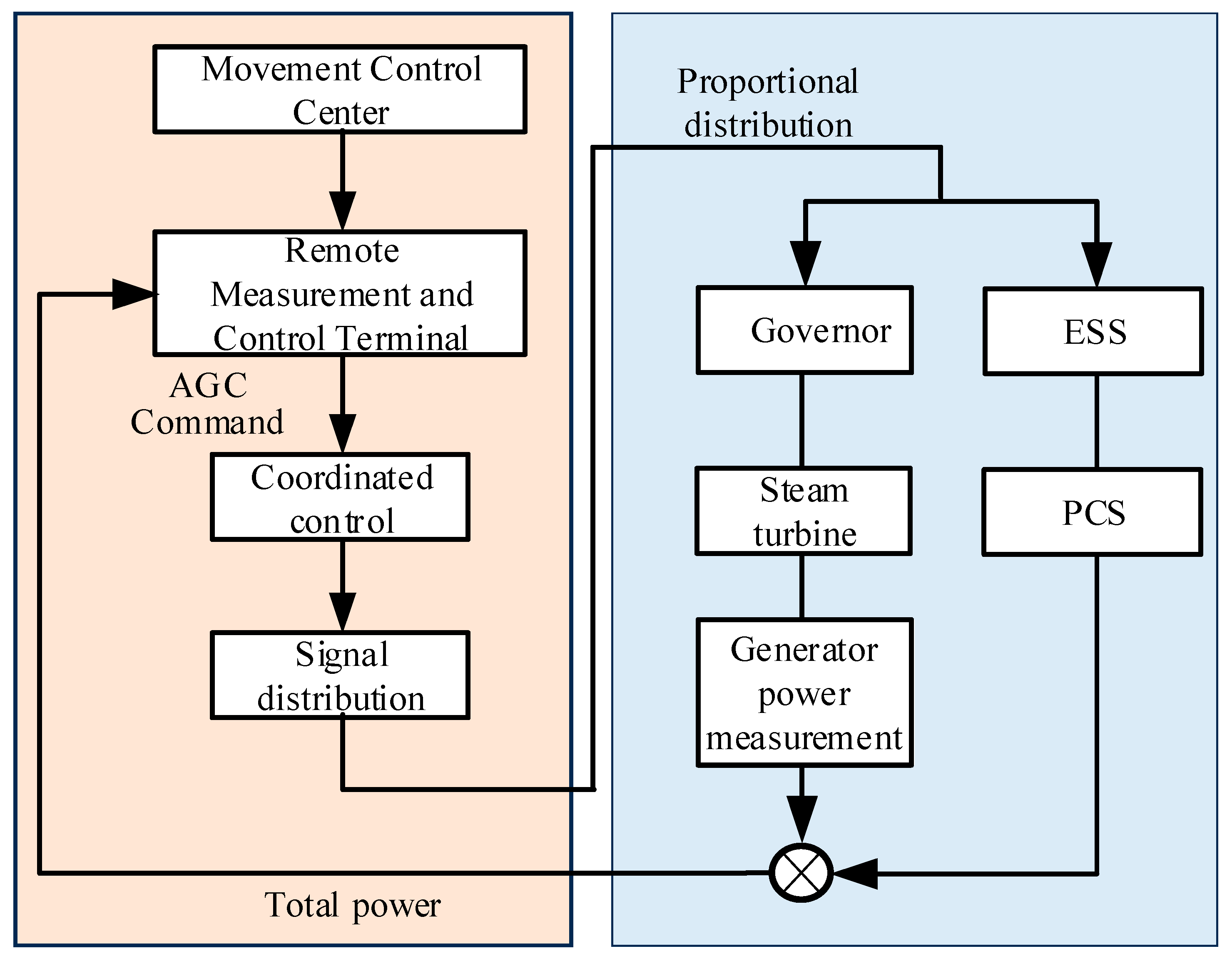
2.1. Hydro-Storage Joint Frequency Regulation Mechanism

In the hydro-storage joint frequency regulation system, hydropower units are directly connected to the grid via transformers, while energy storage is integrated through a power conversion system (PCS) to jointly output power or regulate system frequency fluctuations. In practice, there are always second- or minute-level random active power imbalances between generation output and load demand. The dispatch center monitors the area control error (ACE) signal of the regional grid and inputs it into the AGC system, which issues active power adjustment commands to various frequency regulation units to maintain system frequency stability. The fast response and high charge–discharge cycle capabilities of energy storage can compensate for the limitations of hydropower units in meeting grid frequency regulation demands, achieving complementary advantages. Considering the capacity limitations of storage, in the hydro-storage joint system, large-capacity hydro units act as the primary response units, while the rapid-response storage system serves as a supplementary unit. Figure 1 illustrates a typical secondary frequency regulation structure for the coordinated operation of conventional units and energy storage.

As shown in Figure 1, the remote monitoring and control terminal collects the ACE signal and transmits it to the AGC, which sends active power adjustment commands to the frequency regulation units to improve system frequency and suppress ACE. For hydropower units, they adjust the steam output from the boiler and the valve opening of the turbine according to the AGC commands to change the output power. The energy storage system responds to AGC commands via the PCS.

2.2. Modeling Frequency Response in the Hydro-Storage Joint Frequency Regulation System

This section develops a dynamic response model for secondary frequency regulation in the hydro-storage joint system using the area equivalent method of frequency response, as illustrated in Figure 2. It is assumed that the system employs the flat frequency control (FFC) mode [23], which is commonly used in current power grids. Flat frequency control aims to maintain the system frequency near a predetermined reference value by adjusting the generator’s output power, with the goal of zero frequency deviation.

In Figure 2, $\mathrm{\Delta }f$ represents the power system frequency deviation; $\mathsf{\Delta }{P}_{\mathrm{HG}}$ denotes the output power deviation of the hydro unit; and $\mathsf{\Delta }{P}_{\mathrm{ESS}}$ indicates the output power deviation of the storage system. $\mathsf{\Delta }{P}_{\mathrm{HG}}^{\mathrm{ref}}$ and $\mathsf{\Delta }{P}_{\mathrm{ESS}}^{\mathrm{ref}}$ are the frequency control references for the hydro unit and storage, respectively; while $\mathsf{\Delta }{P}_{\mathrm{L}}$ represents the load change in the system. $\beta$ denotes the frequency bias coefficient of the control area; and $R_{\mathrm{HG}}$ is the droop coefficient of the hydro unit’s governor.${\alpha }_{\mathrm{HG}}$ and ${\alpha }_{\mathrm{ESS}}$ are the power distribution coefficients for the hydro unit and storage, respectively. $T_{\mathrm{G}}$ and $T_W$ represent the time constants of the governor and water hammer effect; $T_{ESS}$ represent the time constants of the storage; while D and M are the load damping coefficient and system inertia constant, respectively. $K_{\mathrm{i}}$ represent the coefficients of the PI control; $\mathrm{\Delta }{P}_{tie}$ denotes the tie-line power transfer; $\mathrm{\Delta }{f}_i$ represents the area i power system frequency deviation; and $T$ represent the coefficient of synchronous torque.

The AGC control system collects the actual frequency deviation and converts it into the ACE signal. The AGC controller then allocates the frequency signal to conventional units and storage systems with rapid frequency response. The frequency regulation power command is distributed to each unit according to the power distribution coefficients. Each frequency regulation unit adjusts its power output upon receiving the command to mitigate frequency fluctuations caused by renewable energy output and load changes. Based on the above process, and in conjunction with Figure 1, $\mathrm{\Delta }f$ can be expressed as follows.

$$\mathrm{\Delta }f(s)={\displaystyle \frac{\mathrm{\Delta }{P}_{\mathrm{HG}}(s)+\mathrm{\Delta }{P}_{\mathrm{ESS}}(s)-\mathrm{\Delta }{P}_{\mathrm{L}}(s)}{sM+D}}$$

(1)

Considering the participation of energy storage in secondary frequency regulation of the grid, the ACE signal, which represents the area frequency deviation, is calculated and allocated according to specific principles to be responded to by battery storage and conventional frequency regulation units. The control model is as follows.

$$\mathrm{ACE}(s)=\mathrm{\Delta }{P}_{\mathrm{T}}(s)+\beta \mathrm{\Delta }f(s)$$

(2)

$${\mathrm{ACE}}_{\mathrm{HG}}(s)={\alpha }_{\mathrm{HG}}\mathrm{ACE}(s)$$

(3)

$${\mathrm{ACE}}_{\mathrm{ESS}}(s)={\alpha }_{\mathrm{ESS}}\mathrm{ACE}(s)$$

(4)

$${\alpha }_{\mathrm{HG}}={\displaystyle \frac{P_{\mathrm{HG}}}{P_{\mathrm{HG}}+P_{\mathrm{ESS}}}}$$

(5)

$${\alpha }_{\mathrm{ESS}}={\displaystyle \frac{P_{\mathrm{ESS}}}{P_{\mathrm{HG}}+P_{\mathrm{ESS}}}}$$

(6)

In the Equations, $\mathrm{ACE}(s)$ represents the regional power deviation; ${\mathrm{ACE}}_{\mathrm{HG}}(s)$ denotes the secondary frequency regulation signal of hydropower units; ${\mathrm{ACE}}_{\mathrm{ESS}}(s)$ stands for the secondary frequency regulation signal of battery energy storage; $P_{\mathrm{HG}}$ signifies the frequency regulation reserve capacity of hydropower units; and $P_{\mathrm{ESS}}$ indicates the frequency regulation reserve capacity of energy storage.

According to the ACE signal allocation principle, the output of hydropower units $P_{\mathrm{CG}}$ and the output of energy storage $P_{\mathrm{ESS}}$ are expressed as follows:

$$\mathrm{\Delta }{P}_{\mathrm{HG}}(s)=-[{\displaystyle \frac{\mathrm{\Delta }f(s)}{R_{\mathrm{HG}}}}+\left(K_{\mathrm{i}}/s\right){\mathrm{ACE}}_{\mathrm{HG}}(s)]G_{\mathrm{HG}}(s)]$$

(7)

$$\mathrm{\Delta }{P}_{\mathrm{ESS}}(s)=-(K_{\mathrm{i}}/s){\mathrm{ACE}}_{\mathrm{ESS}}(s)G_{\mathrm{ESS}}(s)$$

(8)

where $G_{\mathrm{HG}}(s)$ denotes the transfer function model of hydropower units; and $G_{\mathrm{ESS}}(s)$ represents the transfer function model of energy storage batteries.

The root mean square error of system area control deviation is adopted as the evaluation criterion for the effectiveness of secondary frequency regulation, calculated by the following formula:

$${\mathrm{ACE}}_{\mathrm{RMSE}}=\sqrt{{\displaystyle \frac{1}{n}}{\displaystyle \sum _{i=1}^n{({\mathrm{ACE}}_{\mathrm{i}}-{\mathrm{ACE}}_0)}^2}}$$

(9)

where is the ACE value at the i th sampling point; ${\mathrm{ACE}}_0$ is the rated ACE value; and n is the number of sampling points. A smaller ${\mathrm{ACE}}_{\mathrm{RMSE}}$ value indicates less grid frequency fluctuation and better frequency regulation effectiveness.

3. Marginal Rate of Substitution (MRS) Effect in the Frequency
Regulation of the Integrated System

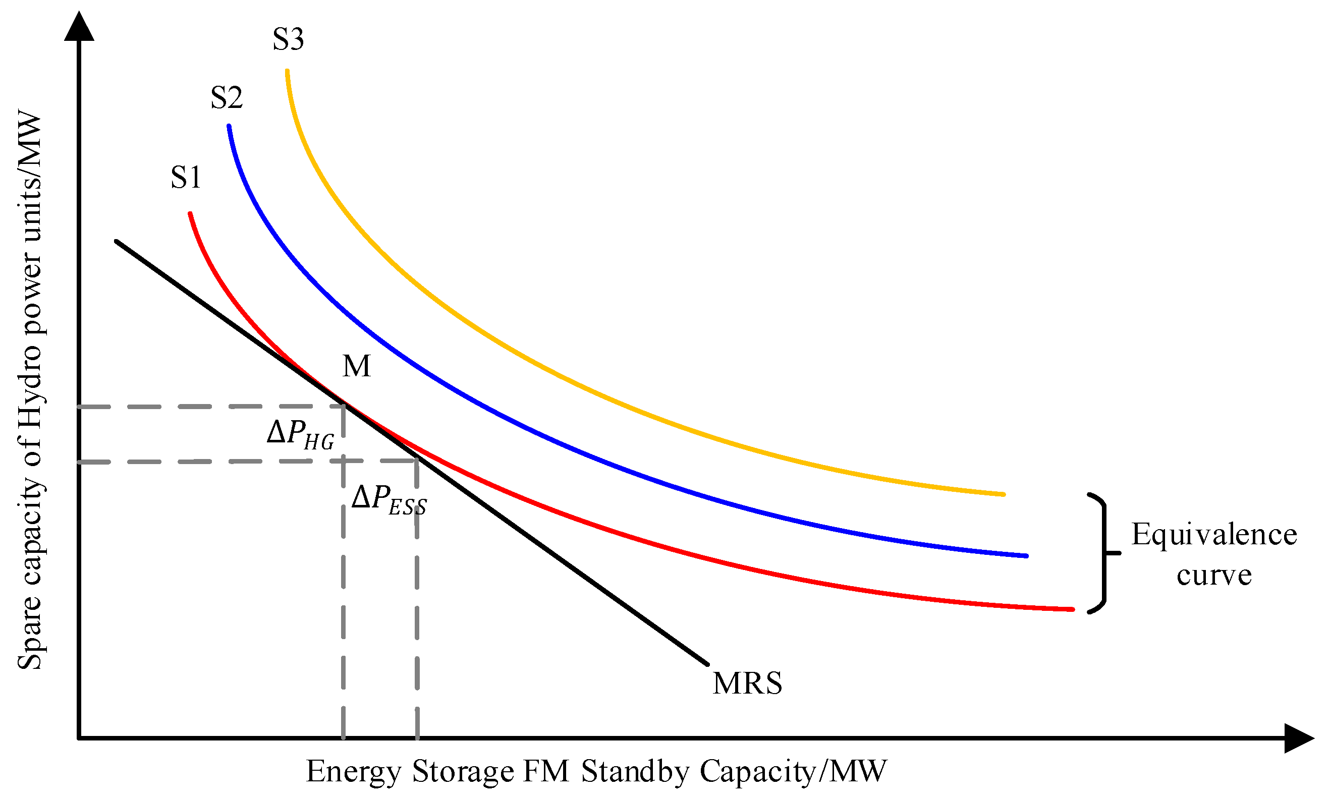
3.1. Marginal Substitution Effect

The marginal rate of substitution (MRS) effect, as an economic concept, characterizes the scenario where increasing the input of one factor by one unit can substitute for a certain quantity of another factor while keeping production demands constant [24].

The marginal substitution curve is a graphical representation constructed based on the marginal substitution effect, which can be used to describe the technical substitution relationship between different production factors. It illustrates how to adjust the proportions of two production factors in production to maintain output constant. The marginal substitution curve is typically derived based on isoquants, and their relationship is depicted in Figure 3. Isoquants are used in economics to represent the amount of one production factor that needs to decrease when the input of another production factor increases to maintain a constant level of utility [24,25]. This curve reveals the objective substitution relationship between production factors, demonstrating a state of “equivalent benefit” for the production factor combination, where each point on the curve has the same utility level. The movement of points on the isoquant curve represents changes in the commodity combination, while utility remains constant, reflecting the competitive relationship between the two production factors. The marginal rate of substitution at each point is the negative slope of the tangent line, indicating the relative value between the two production factors under the current circumstances and their objective substitution relationship. In general, isoquants are an important tool for analyzing decision-making behavior and the substitution relationship between production factors.

In this paper, the marginal substitution effect is extended to the context of the joint frequency regulation of the hydro-energy storage system. This refers to the scenario where, while ensuring the same frequency regulation performance evaluation criteria are met, a certain amount of energy storage frequency regulation reserve can replace the frequency regulation reserve of hydropower units. Subsequently, based on the optimal capacity allocation combination calculated by the marginal substitution effect, the distribution coefficients of hydropower units and energy storage are adjusted, and the frequency regulation output of hydropower units and energy storage is modified to reduce the system’s demand for frequency regulation resources of hydropower units. Figure 3 presents three equivalence curves obtained under different frequency regulation performances, with each curve achieving the same up-regulation performance, generated by the combined frequency regulation reserve capacities of hydropower and energy storage.

According to the isoquant curve in Figure 3, the point of marginal substitution rate equivalence on the curve is denoted by M and can be defined as the negative value of the slope at the equivalence point. Additionally, the reserve capacity for primary frequency control of conventional hydro units is defined as $\mathrm{\Delta }{P}_{\mathrm{HG}}$, and the reserve capacity for frequency control of energy storage is denoted as $\mathrm{\Delta }{P}_{\mathrm{ESS}}$. For any point on the isoquant curve, the slope remains constant; i.e., $\mathrm{\Delta }{S}_1=0$. Therefore, through linearization, it can be derived as follows.

$$\mathrm{\Delta }{S}_1\approx {\displaystyle \frac{\partial S_1}{\partial P_{\mathrm{HG}}}}\mathrm{\Delta }{P}_{\mathrm{HG}}+{\displaystyle \frac{\partial S_1}{\partial P_{\mathrm{ESS}}}}\mathrm{\Delta }{P}_{\mathrm{ESS}}=0$$

(10)

$${\displaystyle \frac{\partial S_1}{\partial P_{\mathrm{HG}}}}\mathrm{\Delta }{P}_{\mathrm{HG}}=-{\displaystyle \frac{\partial S_1}{\partial P_{\mathrm{ESS}}}}\mathrm{\Delta }{P}_{\mathrm{ESS}}$$

(11)

The slope at the equivalence point can be calculated as follows.

$${\left.{\displaystyle \frac{\mathrm{\Delta }{P}_{\mathrm{HG}}}{\mathrm{\Delta }{P}_{\mathrm{ESS}}}}\right|}_{\mathrm{\Delta }{S}_1=0}=-{\displaystyle \frac{\partial P_{\mathrm{ESS}}}{\partial P_{\mathrm{HG}}}}$$

(12)

Since the marginal rate of substitution can be expressed as the negative value of the slope at the equivalence point, the following applies.

$$MR{S}_{\mathrm{HG},\mathrm{ESS}}=-{\left.{\displaystyle \frac{\mathrm{\Delta }{P}_{\mathrm{HG}}}{\mathrm{\Delta }{P}_{\mathrm{ESS}}}}\right|}_{\mathrm{\Delta }{S}_1=0}={\displaystyle \frac{\partial P_{\mathrm{ESS}}}{\partial P_{\mathrm{HG}}}}$$

(13)

3.2. Acquisition of Marginal Substitution Curve for Hydro-Energy Storage Frequency Regulation

Based on the described hydro-energy storage joint system frequency regulation model and evaluation indicators in the previous section, the range of frequency regulation capacity is set, and the combination of frequency regulation capacities of hydropower units and energy storage is altered. The capacity combination of hydropower units and energy storage frequency regulation resources is gradually increased in certain proportions. Through simulation analysis, the ${\mathrm{ACE}}_{\mathrm{RMSE}}$ value is calculated, resulting in a discrete data set regarding different capacity combinations of conventional units and energy storage. Subsequently, the combination data corresponding to the optimal evaluation indicator is selected, and the equivalence curve is fitted. Fitting methods include polynomial fitting and exponential fitting. This paper considers using a segmented fitting method to generate the equivalence curve from the perspective of balance accuracy and complexity. The specific process is as follows.

The x-axis is adaptively divided into multiple intervals, with each interval’s data approximated by a quadratic function. By utilizing the calculation method of the marginal substitution curve from the previous section, the marginal substitution technical function curve for energy storage replacing conventional units is obtained. The marginal substitution function can reflect the capacity of energy storage participating in frequency regulation that can replace the frequency regulation capacity of conventional units, thereby reducing the total frequency regulation capacity. The following sections will detail the methods for obtaining operational data and fitting the marginal substitution curve.

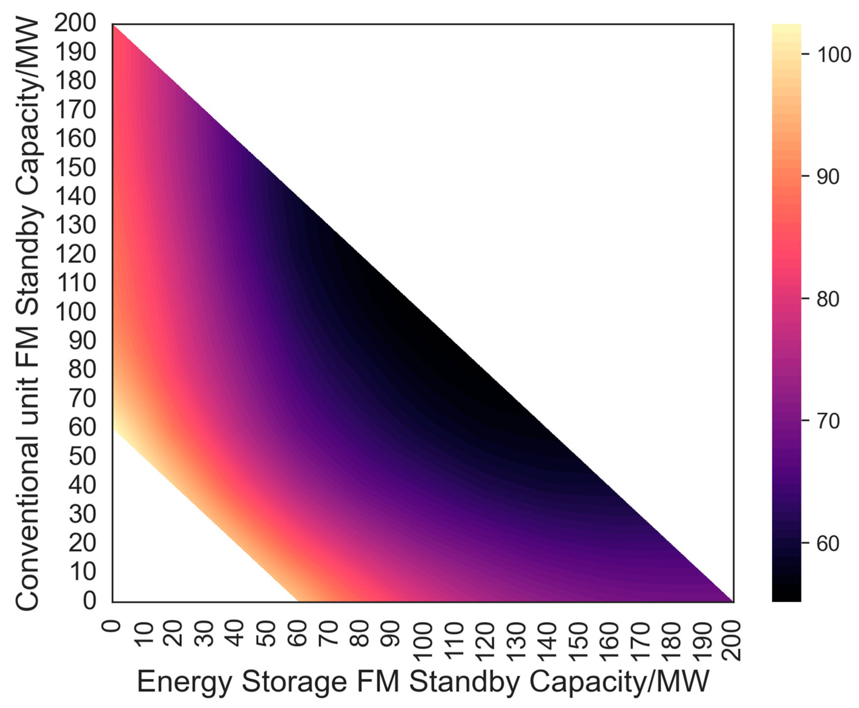
3.3. Operational Data Acquisition Method Based on Gaussian Process Regression

Obtaining a discrete dataset of different capacity combinations for conventional units and energy storage through simulation requires a large amount of data to generate an accurate equivalence curve, making the simulation process both complex and time-consuming. To address this challenge, this study selects key data points as a training set and employs GPR to expand the dataset and generate the marginal substitution curve. GPR not only flexibly models the data but also quantifies the uncertainty in the predictions, thereby demonstrating strong generality and practical applicability. Specifically, Gaussian process regression predicts the observed values based on prior knowledge [26], with its properties determined by the mean function and the covariance function, expressed as follows:

$$m(x)=\mathbb{E}[f(x)]$$

(14)

$$k(x,x^{\prime })=\mathbb{E}[(f(x)-m(x))(f(x^{\prime })-m(x^{\prime }))]$$

(15)

where $x$ and $x^{\prime }$ represent two different input samples; $f(\cdot )$ is the function to be estimated; the covariance function $k(x,x^{\prime })$ is used to represent the covariance between $x$ and $x^{\prime }$, allowing the model to effectively capture the correlations between inputs, including linear or nonlinear dependency structures; and $m(x)$ is the mean function, usually represented in the form of the following polynomial function:

$$m(x,\beta )=H(x)\cdot \beta$$

(16)

where $H(x)$ is a series of basis functions. For example, for an n-dimensional vector $x_i=[x_{i1},\dots x_{in}]$, its linear basis function is $H(x_i)=[1,x_{i1},x_{i2},\dots ,x_{in}]$, and the pure quadratic basis function is $H(x_i)=[1,x_{i1},x_{i2},\dots ,x_{in},x_{i1}^2,x_{i2}^2,\dots ,x_{in}^2]$. $\beta$ is a vector of hyperparameters. Therefore, this real-valued Gaussian process can be expressed as follows.

$$f(x)~\mathcal{G}\mathcal{P}(m(x),k(x,x^{\prime }))$$

(17)

The covariance function $k(x,x^{\prime })$ in Gaussian processes, also known as the kernel function, allows the model to effectively capture the correlations between inputs, including linear or nonlinear dependency structures. This paper adopts the squared exponential (SE) kernel function [27], which has a specific form:

$$k_{\mathrm{SE}}(x,x^{\prime })={\sigma }_f^2\exp [-{\displaystyle \frac{1}{2l^2}}{(x-x^{\prime })}^2]$$

(18)

where ${\sigma }_f$ and $l$ are hyperparameters in the kernel function. From Equation (18), it can be inferred that variables with stronger correlation exhibit more similar properties in their parameter space. Given a training sample set $D=\{(x_i,y_i)|i=1,2,\dots ,n\}=\{X,y\}$, where $x_i\in {ℝ}^d$ represents the d-dimensional input variables and $y_i\in ℝ$ is the output variable corresponding to the input variable. For a regression problem in the form of Equation (13), the prior distribution of the GPR model output vector $y$ is as follows:

$$y~\mathcal{N}(m(x),K(X,X)+{\sigma }_n^{2}I)$$

(19)

where I is a unit vector; and $K(X,X)$ is the covariance matrix composed of multiple kernel functions, taking the following form.

$$K(X,X)=\left[\begin{array}{cccc}k(x_1,x_1)& k(x_1,x_2)& \cdots & k(x_1,x_n)\\ k(x_2,x_1)& k(x_2,x_2)& \cdots & k(x_2,x_n)\\ ⋮& ⋮& \ddots & ⋮\\ k(x_n,x_1)& k(x_n,x_2)& \cdots & k(x_n,x_n)\end{array}\right]$$

(20)

Let $X_{\ast }$ be the input vector in the test set; then, the corresponding random variable $y_{\ast }=f(X_{\ast })$ follows a normal distribution: $y_{\ast }~\mathcal{N}(m(X_{\ast }),K(X_{\ast },X_{\ast }))$. Within the framework of the GPR model, the observed values in the training set $y$ and the predicted values for the test samples $y_{\ast }$ follow a multivariate Gaussian distribution.

$$\left[\begin{array}{c}y\\ y_{\ast }\end{array}\right]~\mathcal{N}(\left[\begin{array}{c}m(X)\\ m(X_{\ast })\end{array}\right],\left[\begin{array}{cc}K(X,X)+{\sigma }_n^{2}I& K(X,X_{\ast })\\ K(X_{\ast },X)& K(X_{\ast },X_{\ast })\end{array}\right])$$

(21)

For the multivariate normal distribution in Equation (21), the posterior distribution of the predicted values $y_{\ast }$ is as follows:

$$\left\{\begin{array}{l}p(y_{\ast }\mid X,X_{\ast },y)~\mathcal{N}(\mu (X_{\ast }),\mathrm{\Sigma }(X_{\ast }))\\ \mu (X_{\ast })=K(X_{\ast },X){[K(X,X)+{\sigma }_n^{2}I]}^{-1}y\\ \mathrm{\Sigma }(X_{\ast })=K(X_{\ast },X_{\ast })-\\ K(X_{\ast },X){[K(X,X)+{\sigma }_n^{2}I]}^{-1}K(X,X_{\ast })\end{array}\right.$$

(22)

where $\mu (X_{\ast })$ is the predicted value of the GPR model, and $\mathrm{\Sigma }(X_{\ast })$ is the prediction output error of the model representing the confidence level of the model prediction.

The specific steps for obtaining operational data based on Gaussian process regression are as follows:

(1)

Prepare training and testing data: According to the model in Section 2.2, a two-dimensional grid data regarding the frequency regulation reserve capacity of hydropower units and energy storage is generated, with the output values being the RMSE values corresponding to the grid data. A small number of obtained data points are used as the training set.

(2)

Create and train the Gaussian process regression model: The function receives the training data and defines a Gaussian process regression model using an exponential kernel. The model is trained to minimize loss, and the function returns the trained model.

(3)

Generate larger grid point data and define and use the model to predict unknown values in the grid points: The function receives the trained model and prediction data and performs predictions.

(4)

Through Gaussian process regression, more data points can be obtained for generating the equivalence curve.

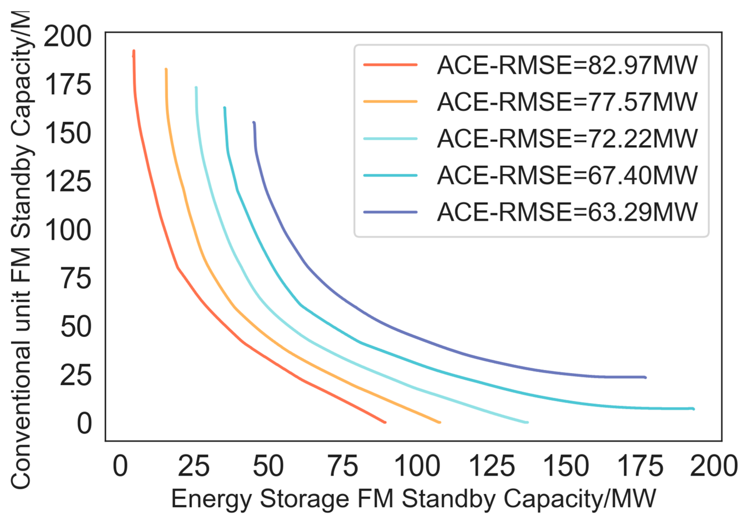
3.4. Generating Marginal Replacement Curves Based on Operational Data Sets

In order to more accurately depict the marginal replacement relationship between energy storage and hydropower units’ frequency regulation effects, the method of least squares is employed to fit the marginal replacement curve. By using the least squares method, fitting is performed with polynomials of different degrees. Here, x and y represent the frequency regulation capacity of energy storage and conventional generating units, respectively. Multiple sets of data obtained from simulations are utilized to calculate the root mean square error (RMSE) of the area control error (ACE). Based on the RMSE of ACE, a set of data can be extracted to determine the tentative functional relationship between x and y.

Before determining the functional relationship, the interval of x is divided into n segments. For each segment, polynomial functions are used for fitting. The functional relationship between the frequency regulation capacity of energy storage x and the frequency regulation capacity of conventional generating units y for each segment is represented by the following quadratic polynomial equation.

$$y=a{x}^2+bx+c$$

(23)

The objective of the least squares method is to find a set of parameters that minimizes the sum of squared residuals between the predicted values and the actual values. For segmented quadratic polynomial fitting, this means applying the least squares method independently to each segment to find the optimal parameters. For each segment, the residual sum of squares (RSS) can be expressed as follows:

$$RSS={\sum }_{i-1}^m{\left(y_i-\left(a{x}_i^2+b{x}_i+c\right)\right)}^2$$

(24)

where m is the number of data points in that segment, and y_i and x_i are the actual value and the corresponding independent variable value for each data point.

To find the parameters a, b, and c that minimize the residual sum of squares, the partial derivatives of the RSS with respect to these parameters are set to zero.

$${\displaystyle \frac{\partial RSS}{\partial a}}=-2{\sum }_{i-1}^n{x}_i^2\left(y_i-\left(a{x}_i^2+b{x}_i+c\right)\right)=0$$

(25)

$${\displaystyle \frac{\partial RSS}{\partial b}}=-2{\sum }_{i-1}^n{x}_i\left(y_i-\left(a{x}_i^2+b{x}_i+c\right)\right)=0$$

(26)

$${\displaystyle \frac{\partial RSS}{\partial c}}=-2{\sum }_{i-1}^n\left(y_i-\left(a{x}_i^2+b{x}_i+c\right)\right)=0$$

(27)

Solving this system of linear equations yields the optimal fitting parameters a, b, and c for each segment.

4. Power System Frequency Regulation Reserve Configuration Method Based on Marginal Replacement

4.1. Cost Model of Hydropower Frequency Regulation

The calculation of the frequency regulation cost of hydropower units is primarily derived by the ratio of the frequency regulation reserve capacity to the total capacity of the hydropower units. The cost of hydropower units consists of investment cost, equipment renewal cost, and additional environmental cost.

$$C_G=\left(C_{\mathrm{Tin}}+C_{\mathrm{Tpre}}+C_{\mathrm{Tae}}\right)·{\displaystyle \frac{P_{\mathrm{f}}}{P_{\mathrm{tol}}}}$$

(28)

where $C_G$ is the frequency regulation cost of hydropower units; $C_{\mathrm{Tin}}$ is the initial investment cost of hydropower units; $C_{\mathrm{Tpre}}$ is the equipment renewal cost of hydropower units; $C_{\mathrm{Tae}}$ is the additional environmental cost; $P_{\mathrm{f}}$ is the frequency regulation reserve capacity; and $P_{\mathrm{tol}}$ is the total capacity of hydropower units.

The investment cost of hydropower units includes construction costs, fuel costs, and maintenance costs.

$$\begin{array}{cc}{C}_{\mathrm{Tin}}\hfill & =C_{\mathrm{d}}+C_{\mathrm{f}}+C_{\mathrm{m}}\hfill \\ & =\left(I_{\mathrm{T}}-S\right)+{\sum }_{n=1}^n\left[{\displaystyle \frac{F\left(n\right)}{{(1+i)}^n}}\right]+{\sum }_{n=1}^n\left[{\displaystyle \frac{M\left(n\right)}{{(1+i)}^n}}\right]\hfill \end{array}$$

(29)

where $C_{\mathrm{d}}$ is the construction cost of hydropower units; $C_{\mathrm{f}}$ is the fuel cost of the units; $C_{\mathrm{m}}$ is the operation and maintenance cost of the units; $I_{\mathrm{T}}$ is the initial investment of hydropower units; S is the residual value of the units; $F\left(n\right)$ is the fuel cost over n years; $M\left(n\right)$ is the annual operation and maintenance cost of the units over n years; i is the interest rate or discount rate; and n is the operating life of the units, typically set at 20 years domestically.

The equipment renewal cost of hydropower units is as follows:

$$C_{\mathrm{Tpre}}=n\cdot \left(C_{\mathrm{r},1}+C_{\mathrm{a}}\right)$$

(30)

where $C_{r,1}$ is the average annual renewal cost of the units; and $C_{\mathrm{a}}$ is the cost of annually adding other auxiliary equipment.

According to relevant policies, power generation companies are required to pay environmental protection taxes for emitting pollutants into the environment. Specifically for hydropower units, emissions of sulfur dioxide (SO₂) and nitrogen oxides (NO_x) into the atmosphere are the main subjects for environmental protection tax collection. The calculation of the environmental protection tax is based on emission levels and policy regulations, with the following formula.

$$\left\{\begin{array}{l}{H}_{\mathrm{S}}=q_{\mathrm{s}}\left(1-{\eta }_{\mathrm{s}}\right)\hfill \\ H_{\mathrm{N}}=q_{\mathrm{n}}\left(1-{\eta }_{\mathrm{n}}\right)\hfill \end{array}\right.$$

(31)

Therefore, the additional environmental cost of hydropower units is as follows:

$$C_{\mathrm{Tae}}=K\left(H_{i,}^s+H_{i,i}^N\right)$$

(32)

where $K$ is the tax amount to be paid per unit of pollution; $H_{\mathrm{S}}$ and $H_{\mathrm{N}}$ are the emissions of SO₂ and NO_x, respectively; $q_{\mathrm{s}}$ and $q_{\mathrm{n}}$ are the amounts of SO₂ and NO_x produced per unit of coal combustion; and ${\eta }_{\mathrm{s}}$ and ${\eta }_{\mathrm{n}}$ are the emission reduction efficiencies of SO₂ and NO_x environmental protection devices of the units.

4.2. Economic Cost Model of Energy Storage Frequency Regulation

The cost of energy storage frequency regulation mainly consists of initial investment cost, equipment renewal cost, operation and maintenance cost, recovery cost, and equipment residual value:

$$C_{\mathrm{ESS}}=C_{\mathrm{Ein}}+C_{\mathrm{Epre}}+C_{\mathrm{Eom}}+C_{\mathrm{Erec}}+C_{\mathrm{Esv}}$$

(33)

where $C_{\mathrm{Ein}}$ is the initial investment cost of energy storage; $C_{\mathrm{Epre}}$ is the equipment renewal cost; $C_{\mathrm{Eom}}$ is the operation and maintenance cost; $C_{\mathrm{Erec}}$ is the recovery cost; and $C_{\mathrm{Esv}}$ is the residual value of the energy storage equipment.

The initial investment cost of energy storage is as follows:

$$C_{\mathrm{Ein}}=k_{pi}{P}_{\mathrm{HN}}+k_{ei}{E}_{\mathrm{HN}}$$

(34)

where $k_{pi}$ is the initial investment cost per unit power; $k_{ei}$ is the initial investment cost per unit capacity; $P_{\mathrm{HN}}$ is the rated power of the energy storage; and $E_{\mathrm{HN}}$ is the rated capacity of the energy storage.

The equipment renewal cost of energy storage is as follows:

$$C_{\mathrm{Epre}}={\displaystyle \sum }_{k=1}^n\left(k_{pp}{P}_{\mathrm{HN}}+k_{\mathrm{ep}}{E}_{\mathrm{HN}}\right){(1+r)}^{-{\displaystyle \frac{kT}{n+1}}}$$

(35)

where $k_{pp}$ is the replacement cost per unit power; $k_{\mathrm{ep}}$ is the replacement cost per unit capacity; T is the engineering service life; and n is the number of replacements of the energy storage device within the service life, directly impacting the economic cost of the energy storage system. The relationship between the number of replacements of the energy storage device and the battery life can be expressed as follows:

$$n={\displaystyle \frac{T}{S_{\mathrm{BESS}}}}$$

(36)

where $S_{\mathrm{BESS}}$ is the average usage life of the battery energy storage.

The calculation method for the usage life of the battery energy storage is as follows:

$$S_{BESS}={\displaystyle \frac{{\displaystyle \sum _{j=1}^m{N}_{\mathrm{BESS}}(x_j)}}{365}}$$

(37)

where m is the number of discharges per day for the battery; and $N_{\mathrm{BESS}}(x_j)$ is the number of cycles when the discharge depth is $x_j$.

The operation and maintenance cost, recovery cost, and equipment residual value of energy storage are as follows:

$$C_{\mathrm{Eom}}=k_{\mathrm{po}}{P}_{\mathrm{HN}}{\displaystyle \frac{{(1+r)}^T-1}{r{(1+r)}^T}}+{\displaystyle \sum }_{t=1}^T{k}_{eo}{W}_t{(1+r)}^{-t}$$

(38)

$$C_{\mathrm{Erec}}=\left(k_{\mathrm{pr}}{P}_{\mathrm{HN}}+k_{\mathrm{er}}{E}_{\mathrm{HN}}\right)\left(n+1\right){(1+r)}^{-T}$$

(39)

$$C_{\mathrm{Esv}}={\sigma }_{\mathrm{res}}\left(C_{in}+C_{\mathrm{pre}}\right){(1+r)}^{-T}$$

(40)

where $k_{\mathrm{po}}$ and $k_{\mathrm{eo}}$ are the operation and maintenance costs per unit power and per unit capacity; $k_{\mathrm{pr}}$ and $k_{\mathrm{er}}$ are the recovery costs per unit power and per unit capacity; and ${\sigma }_{res}$ is the residual rate.

4.3. Frequency Capacity Optimization Configuration Method with Cost Optimization as the Objective

The marginal replacement characteristics between hydropower units and energy storage frequency regulation capacity provide important reference conditions for analyzing and economically optimizing the frequency capacity configuration while ensuring system frequency regulation safety and stability.

By calculating the revenue curves of the conventional unit frequency regulation cost model and the energy storage frequency regulation cost model, the iso-revenue curve represents the total cost obtained from different combinations of conventional units and energy storage. Its slope represents the cost price ratio between unit conventional unit capacity cost and unit energy storage capacity cost, expressed as follows:

$$C_{\mathrm{tol}}=C_{\mathrm{G}}{P}_{\mathrm{hg}}+C_{ESS}{P}_{\mathrm{ess}}$$

(41)

where $C_{\mathrm{tol}}$ is the total frequency regulation capacity cost; $C_{\mathrm{G}}$ is the unit hydropower unit capacity cost price; and $C_{ESS}$ is the unit energy storage capacity cost price. When the marginal replacement rate equals the cost price ratio, the optimal combination of conventional unit and energy storage input capacity is achieved, i.e.,

$$MR{S}_{\cos t}={\displaystyle \frac{C_{\mathrm{G}}}{C_{ESS}}}$$

(42)

At a certain point on the production transformation curve in Figure 4, where the marginal replacement rate equals the slope of the cost price line, the cost-optimal and best-performing configuration of hydropower units and energy storage frequency reserve is achieved. Point O in the figure represents the optimal configuration point of conventional units and energy storage frequency reserve capacity, also known as the optimal equilibrium point.

Using the marginal replacement effect method to determine the optimal combination of conventional units and energy storage frequency regulation capacity involves the following steps:

(1)

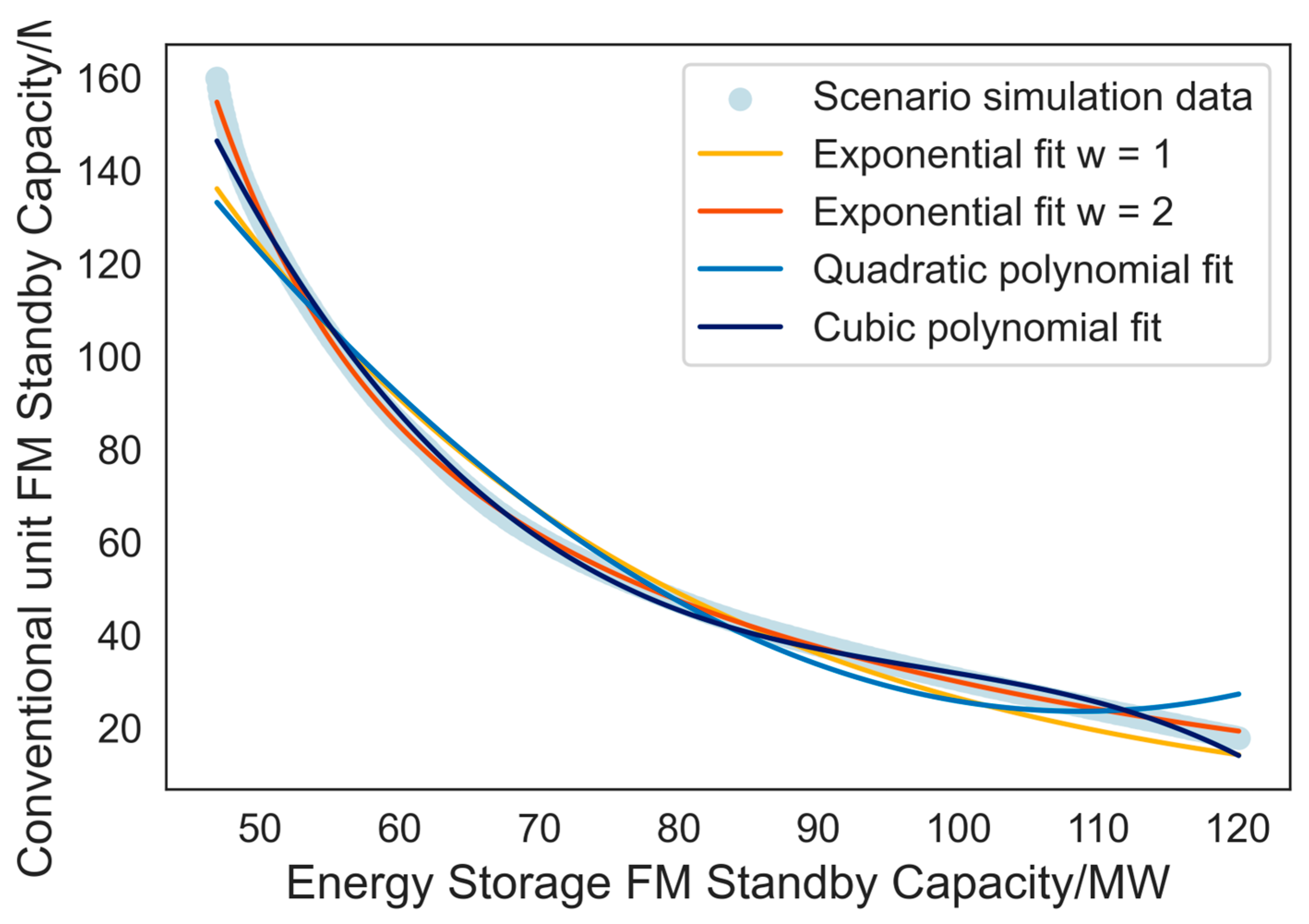
Draw the equivalent curve based on the simulation results of the hydro-energy storage joint frequency regulation system. By varying the ratio of frequency regulation reserve capacity between conventional units and energy storage, obtain the output frequency performance indicators. Based on the dataset, derive the equivalent curve and fit its function expression as $y=f\left(x\right)$.

(2)

Utilize the method for obtaining the marginal replacement curve in Section 2.2 to determine the marginal replacement rate function $y=f\left(x\right)$ for conventional units and energy storage frequency regulation based on the function $y$’.

(3)

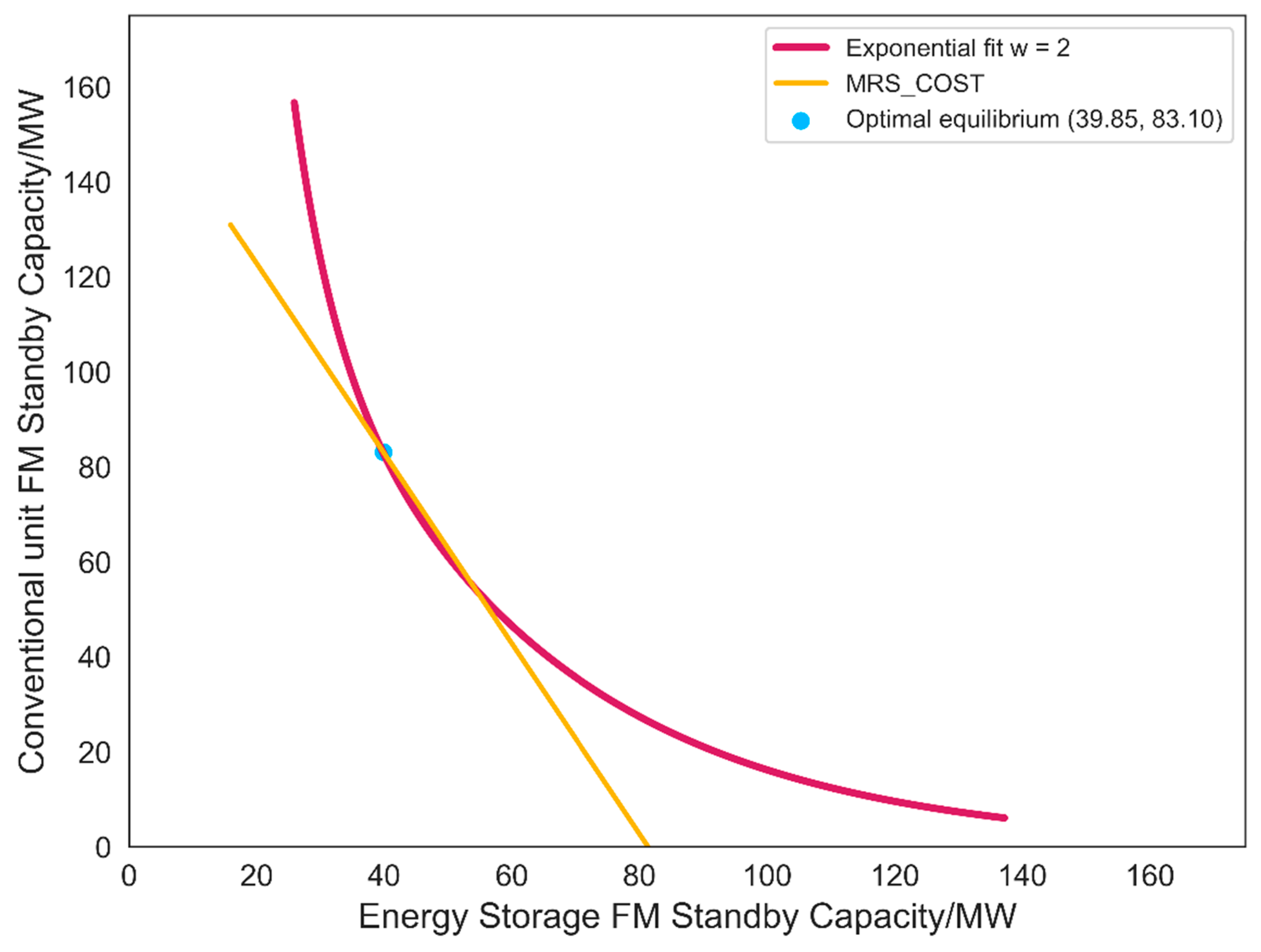
Obtain the iso-revenue line based on the ratio of the price of conventional unit frequency regulation capacity to the price of energy storage frequency regulation capacity $C_{\mathrm{G}}/C_{ESS}$.

(4)

Calculate the marginal replacement rate $MR{S}_{\cos t}$ for the optimal combination of conventional units and energy storage frequency regulation under the minimum cost based on $MR{S}_{\cos t}=C_{\mathrm{G}}/C_{ESS}$.

(5)

By using $MR{S}_{\cos t}$ and the marginal replacement rate function, determine the frequency regulation capacity combinations at the optimal equilibrium points.

5. Case Study

5.1. Test System

To verify the feasibility and effectiveness of the proposed method for configuring the frequency regulation capacity of conventional units and energy storage in regional power systems, this section considers the presence of both reheat-type hydropower units and lithium battery energy storage as two frequency regulation resources. The main parameters are shown in

Table 1. Parameters of the simulation system model.

Model Parameter		Value
Hydropower unit	Active droop coefficient $R_{HG}$	0.5
	Generator speed regulator time constant $T_G$	0.08 s
	Time constant of water hammer effect $T_W$	0.3 s
ESS	Climbing time constant $T_b$	0.01 s
Equivalent system	Equivalent inertia constant $H$	10 MVA·s/MW
	Damping coefficient $D$	1.0 N/m
Control system	Frequency deviation coefficient $\beta$	21.0 MW/Hz
	Proportional control parameters $K_P$	0.822
	Integral control parameters $K_I$	0.16

.

The testing system was simulated and analyzed using the MATLAB/Simulink platform. The simulation system employed the daily load fluctuation curve of an actual power grid, as shown in Figure 5, with a simulation time of 24 h.

In this study, ${\mathrm{ACE}}_{\mathrm{RMSE}}$ is adopted as the metric for frequency quality evaluation. Considering a total frequency regulation capacity range of 20–200 MW in the region, the capacities of thermal units and energy storage are combined in increments of 10 MW. The dataset constructed from Simulink simulation data using a heat map as an analytical tool is shown in Figure 6, with the values corresponding to different colors indicated on the right (in MW). The marginal substitution curve is derived through heat map analysis, thereby determining the required configuration of frequency regulation capacities for the system.

Figure 6 illustrates the impact of different capacity combinations of hydropower units and energy storage on ${\mathrm{ACE}}_{\mathrm{RMSE}}$ in the system. The darkest color indicates the lowest ${\mathrm{ACE}}_{\mathrm{RMSE}}$ produced by the combination of conventional units and energy storage, while the brightest color represents the opposite. The white area represents unconsidered combinations of conventional units and energy storage. Within the given frequency regulation capacity range, as the frequency regulation capacity of energy storage increases, the performance indicator improves. However, beyond a certain value, the performance decreases due to energy storage limitations, reaching the state of energy storage state of charge (SOC) constraints, leading to an increase in ACE. Therefore, energy-limited energy storage resources need to be combined with conventional unit resources.

5.2. Obtaining the Marginal Replacement Curve

After generating the heatmap, in order to create a more accurate equivalent curve, the incremental step size of the data corresponding to the capacity combinations of conventional generators and energy storage was reduced from 20 MW to 0.1 MW to increase the number of data points and generate a more precise equivalent curve. Following the Gaussian process regression method outlined in Section 3.3, a new dataset of interpolated RMSE values for ACE was obtained as shown in Figure 7.

Based on the new dataset, an equivalent curve was generated, as shown in Figure 8. The equivalent curve represents the combinations of hydropower units and energy storage that achieve equal evaluation indicators.

Taking the equivalence curve corresponding to ACE_RMSE = 72.22 MW as an example, exponential, quadratic, and cubic polynomial fitting methods are employed, with the fitted curves presented in Figure 9.

The segmented polynomial fitting method proposed in this paper is applied to the equivalence curve corresponding to ACE_RMSE = 72.22 MW, and the fitting result is shown in Figure 10. Considering the characteristics of the curve, the curve was divided into five intervals, namely, [0, 25], [25, 50], [50, 75], [75, 100], [100, ∞], with each interval fitted using a quadratic function.

From the figure, it can be observed that various forms of fitting methods, including quadratic polynomial fitting, cubic polynomial fitting, and exponential fitting, were compared and analyzed with the method proposed in this paper. The fitting accuracy is shown in

Table 2. Fitting accuracy table.

Fitting Method		RMSE
Index fitting	$\omega =1$	3.38607
	$\omega =2$	1.39663
Quadratic polynomial fitting		6.70638
Cubic polynomial fitting		2.87712
Segmented polynomial fitting		0.03250

, where the proposed segmented fitting method demonstrated the best accuracy with a root mean square error of 0.03250. To ensure fitting accuracy, the number of segments for segmented quadratic fitting is generally not less than four segments, and this paper utilized a five-segment segmented fitting.

The segmented fitting functions obtained through the least squares method are as follows.

$$\left\{\begin{array}{cc}{y}_1=0.15384x^2-26.65437x+624.53690& x\in \left[0,25\right]\\ y_2= 0.11944x^2-12.78043x+401.52898& x\in \left[25,50\right]\\ y_3= 0.01709x^2-3.14739x+173.52481& x\in \left[50,75\right]\\ y_4= 0.001850x^2-0.95738x+94.57905& x\in \left[75,100\right]\\ y_5= 0.00130x^2-0.78989x+83.43932& x\in \left[100,\infty \right]\end{array}\right.$$

(43)

As shown in Figure 10, three random points were selected from the dataset obtained through Gaussian process regression, with coordinates (40.10, 82.26), (59.50, 46.77), (94.60, 20.56), and (132.70, 1.52). The corresponding ACE values for these points were calculated as 74.07, 73.15, 72.78, and 73.86, with an average error rate of 1.72%. It is evident that the accuracy of the operational data obtained based on Gaussian process regression is good.

Using the methodology proposed in this paper, the segmented polynomial fitting functions derived from Figure 10 are combined with Equation (13) to compute the marginal rate of substitution (MRS), thereby generating the marginal substitution curve illustrated in Figure 11.

By conducting regression analysis, the Equation of the curve can be inferred as follows.

$$\left\{\begin{array}{c}MR{S}_1=-1.8162x+49.71733\begin{array}{ccc}& & \end{array}x\in \left[0,25\right]\\ MR{S}_2=-0.19122x+10.05574\begin{array}{ccc}& & \end{array}x\in \left[25,50\right]\\ MR{S}_3=-0.02842x+2.69002\begin{array}{ccc}& & \end{array}x\in \left[50,75\right]\\ MR{S}_4=-0.00512x+1.08951\begin{array}{ccc}& & \end{array}x\in \left[75,100\right]\\ MRT{S}_5=-0.00019x+0.59969\begin{array}{ccc}& & \end{array}x\in \left[100,\infty \right]\end{array}\right.$$

(44)

The marginal substitution curve quantifies the equivalent replacement relationship between energy storage and hydropower units in frequency regulation capacity allocation, establishing a theoretical foundation for multi-resource collaborative optimization. As depicted in Figure 11, when the marginal rate of substitution (MRS) on the y-axis reaches 1.0, 51.60 MW of energy storage capacity substitutes 68.38 MW of hydropower capacity (replacement ratio = 1:1.325) while maintaining equivalent frequency regulation performance. Consequently, the total frequency regulation reserve capacity decreases from 125.00 MW to 108.22 MW, achieving a 13.42%.

5.3. Analysis of Frequency Capacity Optimization Configuration with Cost Optimization as the Objective

Considering the system, the frequency regulation cost of conventional units is 6 million RMB/MW, and the frequency regulation cost of energy storage is 3 million RMB/MW. Therefore, the cost contours of the capacity combinations are linear, as shown in Figure 12.

Figure 13 illustrates the reserve capacity portfolio optimized for minimum cost. By leveraging the iso-revenue line and the equivalent substitution curve of conventional units and energy storage reserve capacities, the intersection point represents the optimal equilibrium of the reserve capacity combination. At this equilibrium point, the energy storage reserve capacity is 39.85 MW, while the conventional unit reserve capacity is 83.10 MW. At this point, while maintaining the marginal substitution rate (MRS), the reserve capacity costs of both energy storage and conventional units are minimized, resulting in a total minimum cost of 618.15 million RMB. In contrast, if only conventional hydropower units participate in frequency reserve, a total capacity of 125 MW is required, incurring a cost of 750 million RMB. Compared to this baseline, the cost-optimized strategy proposed in this study achieves a 17.58% reduction in overall costs.

6. Conclusions

This paper proposes a frequency reserve capacity allocation method for hydropower-energy storage coordinated systems, incorporating the marginal cost effect. By leveraging the intrinsic characteristics of frequency regulation resources, the proposed approach optimizes resource allocation, effectively reducing frequency regulation costs. Simulation results validate the feasibility of the proposed method, leading to the following key conclusions:

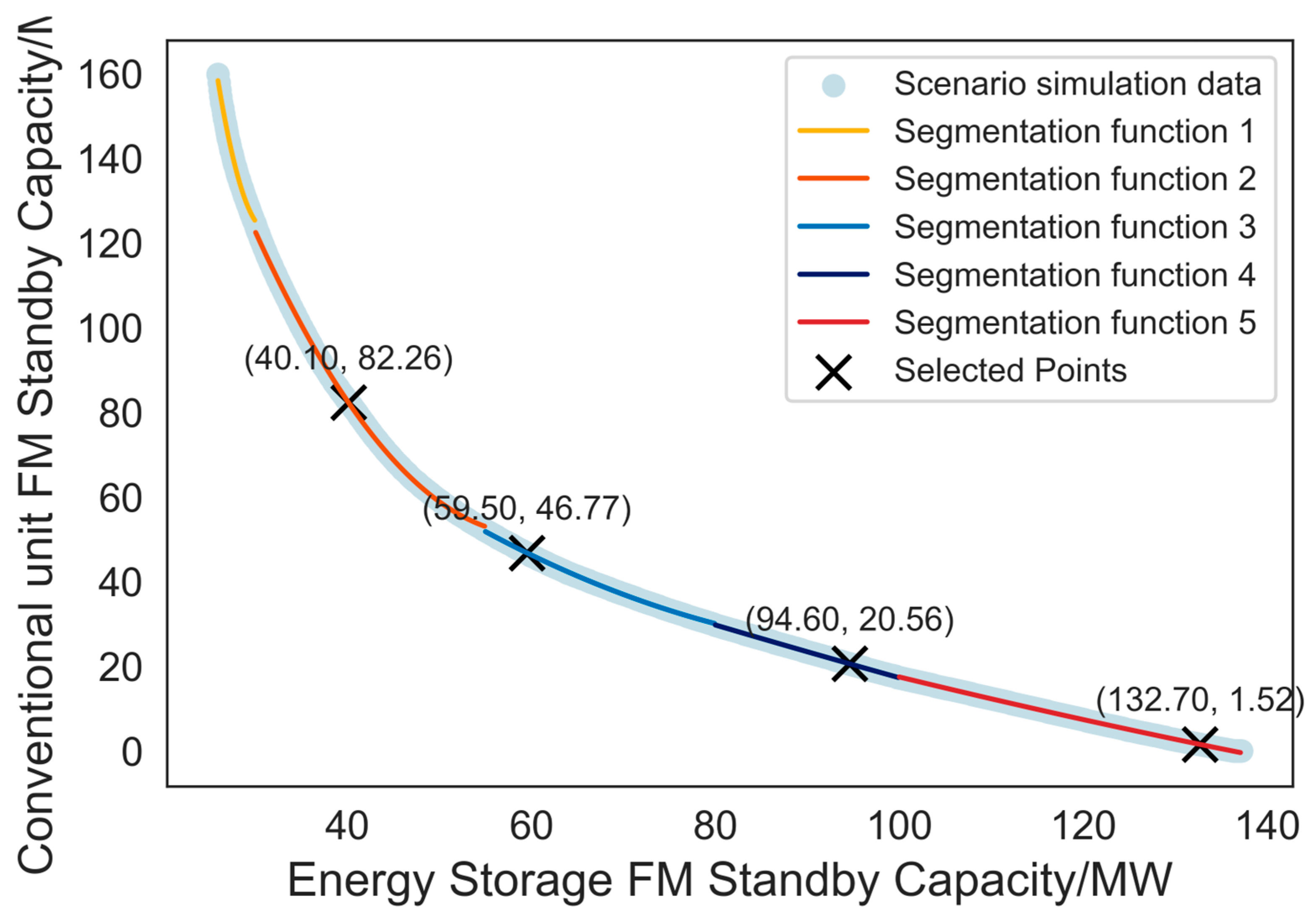
• The proposed operational data acquisition method based on GPR and the segmented fitting approach for equivalent curves significantly reduce the difficulty of data acquisition in terms of data density and time span, without compromising data accuracy. Simultaneously, the proposed method ensures high curve-fitting precision. The error rate of the proposed data acquisition method is 1.72%, while the root mean square error (RMSE) of the proposed curve-fitting method is 0.03250;
• The proposed hydro-storage coordinated frequency regulation reserve configuration method, compared to frequency regulation using a single hydropower unit, achieves the same frequency regulation performance while incorporating the marginal substitution principle. This approach reduces the total frequency regulation reserve capacity from 125 MW to 108.22 MW, representing a 13.42% reduction in capacity. Furthermore, when considering cost factors, the frequency regulation cost decreases from 750 million RMB to 618.15 million RMB, resulting in a 17.58% cost reduction.

Future work will expand this research to the optimization configuration of various frequency resources within a region by incorporating the marginal substitution effects analysis methods from economics.

References

1. Zhang, H.; Zhang, Y.; Ma, Q.; Guo, D. Development trend of new energy industry under the dual carbon goal. Energy Storage Sci. Technol. 2022, 11, 1677–1678. [Google Scholar]
2. Liu, Z.; Peng, D.; Zhao, H.; Wang, D.; Liu, Y. Development prospects of energy storage participating in auxiliary services of power systems under the targets of the dual-carbon goal. Energy Storage Sci. Technol. 2022, 11, 704–716. [Google Scholar]
3. Han, Z.; Ju, P.; Qin, C.; Sun, D.; Sun, H.; Zheng, Y. Review and prospect of research on frequency security of new power system. Electr. Power Autom. Equip. 2023, 43, 112–124. [Google Scholar]
4. Zhao, H.; Wang, W.; Li, X.; Liu, D.; He, C. Day ahead joint trading decision model for electricity, frequency regulation and reserve market considering energy storage participation. Power Syst. Technol. 2023, 47, 4575–4584. [Google Scholar]
5. Zhang, S.; Yuan, B.; Xu, Q.; Zhao, J. Optimal control strategy of secondary frequency regulation for power grid with large-scale energy storages. Electr. Power Autom. Equip. 2019, 39, 82–88, 95. [Google Scholar]
6. Zhou, X.; Zhang, Y.; Ma, X.; Li, G.; Wang, Y.; Hu, C.; Liang, J.; Li, M. Performance characteristics of photovoltaic cold storage under composite control of maximum power tracking and constant voltage per frequency. Appl. Energy 2022, 30, 117–840. [Google Scholar] [CrossRef]
7. Ma, Y.; Hu, Z.; Diao, R. Day-ahead optimization strategy for shared energy storage of renewable energy power stations to provide frequency regulation service. Power Syst. Technol. 2022, 46, 3857–3868. [Google Scholar]
8. Li, B.; Chen, M.; Zhong, H.; Ma, Z.; Liu, D.; He, G. A review of long- term planning of new power systems with large share of renewable energy. Proc. CSEE 2023, 43, 555–580. [Google Scholar]
9. Wang, N.; Li, Z.; Zhou, X.; Liu, C.; An, K.; Cong, L. Characteristics research on combined frequency regulation of AGC and energy storage in power plant and the simulation. Hydro Power Gener. 2021, 50, 148–156. [Google Scholar]
10. Zhu, W.; Zhou, Y.; Xu, Y.; Shi, T. Application and optimization of battery energy storage technology in new energy generation system. Energy Storage Sci. Technol. 2024, 13, 2737–2739. [Google Scholar]
11. Xu, L.; Xu, L.; Song, F. System fault monitoring and diagnostic analysis of electrochemical energy storage power stations. Energy Storage Sci. Technol. 2024, 13, 2788–2790. [Google Scholar]
12. Yang, S.; Lin, W.; Cui, Y.; Wang, E. Analysis and enlightenment of AGC regulation for combined hydro and storage system based on power and capacity compensation. Energy Storage Sci. Technol. 2023, 12, 299–311. [Google Scholar]
13. Xie, D.; Xu, Y.; Li, H.; Jia, X.; Liang, L.; Hong, F. Optimization of Hybrid Energy Storage Capacity Allocation Based on AGC Frequency regulation of Auxiliary hydro power Units. Electr. Eng. 2023, 19, 15–18. [Google Scholar]
14. Zhang, S.; Liu, H.; Wang, F.; Hui, G.; Tianling, S. A balancing control strategy for “power-X-power” energy storage cluster in system load frequency control. Proc. CSEE 2022, 42, 886–898. [Google Scholar]
15. Gao, S.; Li, J.; Song, H.; Ding, L.; Zhang, C. An integrated hydro power energy storage system for improving primary frequency regulation performance of hydro power units. Power Syst. Prot. Control 2023, 51, 116–125. [Google Scholar]
16. Hong, F.; Jia, X.; Liang, L.; Hao, J.; Wang, W.; Fang, F. Research on the integration of flywheel energy storage capacity allocation under hydro-storage coupling cooperative frequency regulation strategy. Hydro Power Gener. 2023, 52, 65–75. [Google Scholar]
17. Toufani, P.; Karakoyun, E.C.; Nadar, E.; Fosso, O.B.; Kocaman, A.S. Optimization of Pumped Hydro Energy Storage Systems under Uncertainty: A Review. J. Energy Storage 2023, 73, 109306. [Google Scholar] [CrossRef]
18. Hederman, W.F. Electricity markets monitoring at the Federal Energy Regulatory Commission. In Proceedings of the 2003 IEEE Power Engineering Society General Meeting, Toronto, ON, Canada, 13–17 July 2003; p. 499. [Google Scholar]
19. Zhao, W.; Li, B.; Wei, H.; Wei, C.; Deng, J. The optimal AGC control strategy considering the primary frequency regulation under the control performance standard for the interconnected power grid. Proc. CSEE 2016, 36, 2656–2664. [Google Scholar]
20. Tang, Z.; Song, S.; Bai, X.; Wang, K. Multi-source FM Capacity Allocation Strategy Based on Master-Slave Game. Sci. Technol. Eng. 2024, 24, 7693–7700. [Google Scholar]
21. Zhang, F.; Li, B.; Ding, L. Parameter setting method of time-varying frequency regulation considering linked energy distribution of wind power for frequency regulation. Autom. Electr. Power Syst. 2022, 46, 1–13. [Google Scholar]
22. Yang, Y.; Wang, D.; Hu, B.; Wang, H.; Luo, H. Multi-source optimal joint frequency regulation control strategy based on improved multi-agent Q-learning. Power Syst. Prot. Control 2022, 50, 135–144. [Google Scholar]
23. Ferguson, C.E.; Gould, J.P. Microeconomic Theory; McGraw-Hill/Irwin: Homewood, IL, USA, 1975. [Google Scholar]
24. Yu, D.; Lo, K.L.; Wang, X.; Wang, X. MRTS traction power supply system simulation using Matlab/Simulink. In Proceedings of the IEEE 55th Vehicular Technology Conference, Birmingham, AL, USA, 6–9 May 2002; Volume 1, pp. 308–312. [Google Scholar]
25. Besanko, D.; Braeutigam, R. Microeconomics; John Wiley & Sons: Hoboken, NJ, USA, 2016. [Google Scholar]
26. Wagh, C.; Shivam, C.; Revati, G.; Shadab, S.; Wagh, S.R. Speed Estimation of Induction Motor Using Gaussian Process Regression. In Proceedings of the 2023 9th International Conference on Control, Decision and Information Technologies (CoDIT), Rome, Italy, 3–6 July 2023; pp. 1–6. [Google Scholar]
27. Li, G.; Lu, W.; Bian, J.; Sun, Y. Probabilistic optimal power flow considering correlation and time series based on adaptive diffusion kernel density estimation. Proc. CSEE 2021, 41, 1655–1663. [Google Scholar]
Figure 1. Control loop of the power system with hydro units and energy storage systems participating in frequency regulation.
Electronics 14 01582 g001
Figure 2. Frequency response model of a combined hydro-energy storage system is considered.
Electronics 14 01582 g002
Figure 3. Equivalent curves of hydropower units and energy storage for frequency regulation.
Electronics 14 01582 g003
Figure 4. Optimal cost allocation method for frequency regulation.
Electronics 14 01582 g004
Figure 5. Daily actual load fluctuation curve for an actual grid.
Electronics 14 01582 g005
Figure 6. Heat map of the dataset.
Electronics 14 01582 g006
Figure 7. Dataset obtained based on the Gaussian regression method.
Electronics 14 01582 g007
Figure 8. Equivalent curve.
Electronics 14 01582 g008
Figure 9. Test cases of different fittings of equivalent curves.
Electronics 14 01582 g009
Figure 10. Piecewise polynomial fitting test case.
Electronics 14 01582 g010
Figure 11. Marginal substitution curve.
Electronics 14 01582 g011
Figure 12. Equal cost line.
Electronics 14 01582 g012
Figure 13. Relationship between the reserve capacity portfolio with the optimal cost as the goal.
Electronics 14 01582 g013