Abstract
This article discusses the safety issues of autonomous vehicles using GNSS when transporting particularly dangerous goods, such as flammable and explosive materials. A method for the special processing of GNSS navigation information is presented, which consists of collecting readings of the relative navigation positions of the vehicle. The novelty of the method lies in the substantiation of the refusal to use a standard speedometer and the study of the minimum permissible vehicle speed, measured exclusively on the basis of the results of processing GNSS data. To confirm the assumptions inherent in the described method, a physical experiment was carried out, the results of which showed that the accuracy of the speedometers of standard vehicles is insufficient to ensure sufficient safety if the required driving speed should not exceed several km/h. The methodological basis for conducting a physical experiment is to measure the sequence of calculations of the coordinates {Xi, Yi}(t), i = 1, 2, … of the vehicle, continuously calculate the vehicle speed in km/h, and use a speed limiting device set to a certain permissible technical state for the transportation of especially dangerous goods.
1. Introduction
Dangerous goods [1] are goods that could be used for terrorist purposes and therefore lead to serious consequences, such as the loss of multiple lives or mass destruction. There is a certain category of goods the transportation of which is regulated by international and national rules [2]. Improving the safety of slow-moving vehicles carrying highly dangerous goods is an important task that requires an integrated approach as follows:
- Equipping vehicles with modern security systems: Anti-lock brakes (ABS), Electronic Stability Control (ESC), a tire pressure monitoring system, rearview cameras and a surround view system, and blind spot sensors;
- The installation of automatic braking and collision warning systems;
- Equipping vehicles with warning devices (flashing lights and sound signals) to warn other road users;
- The use of reinforced body structures to protect the cargo in the event of an accident;
- The implementation of real-time monitoring systems for the condition of the cargo (temperature, pressure, and leaks);
- The use of GNSS to track the route and speed.
The implementation of these measures will significantly reduce the risks associated with the transportation of especially dangerous goods and improve safety for both road users and the environment. The transportation of dangerous goods by road is the subject of analysis and, depending on the potential consequences that may arise in the event of an adverse scenario related to the handling of dangerous goods, these goods are classified into specific categories [3]:
- Explosive;
- Gaseous;
- Flammable solid;
- Spontaneously combustible;
- Organic pyroxides;
- Poisonous, toxic, or infectious;
- Radioactive;
- Corrosive;
- Others [4].
The movement of the vehicle must be carried out along a pre-agreed route, indicating the locations of stops, including those for rest and refueling (gas stations) [5].
AVs used for the transportation of dangerous goods must be equipped with GNSS tracking systems. To attract the attention of other road users, the transportation of dangerous goods is carried out only if there are markings and flashing beacons. Dangerous goods can only be transported on one semi-trailer. When transporting dangerous goods, the transport company must mark the vehicle with the designation of the type of cargo. This is a rhombus at least 15 cm high, with the class at the top and the UN number at the bottom. (Elements of UN Markings—UN Packaging Codes: the UN symbol, packaging identification codes, packaging group level or equivalent information, gross mass or specific gravity, hydrostatic test pressure or solids, the year and location of the manufacturer, and the identification of the manufacturer or approval agency).
In some cases of the transportation of especially dangerous or oversized cargo, it is necessary to reduce the speed of the vehicle to several kilometers per second.
Modern vehicle monitoring systems rely on advanced techniques such as Weigh in Motion (WIM) and High-Speed Weigh in Motion (HS-WIM), which enable the measurement of vehicle mass in motion without disrupting traffic flow. Weigh-in-Motion (WIM) techniques estimate static axle loads indirectly by measuring the vehicle’s dynamic response as it moves over sensors embedded in the road. These methods are cost-effective and easier to implement but are reliable only on smooth surfaces and at low speeds [6,7].
High-Speed Weigh-in-Motion (HS-WIM) systems measure the mass of vehicles at normal speeds without disrupting traffic flow. They use strain gauge sensors to measure pressures and require calibration functions for accuracy. However, these systems have a 10% error margin compared to static loads due to the dynamic interactions [7,8]. The use of dynamic load measurement methods and advanced sensors allows for precise real-time monitoring of vehicle parameters. These technologies are widely applied in fleet management, risk assessment for maneuvers, and driver assistance, all aimed at improving road safety. The time domain method, among various moving-load identification techniques, has been found to be the most effective for incorporation into a moving-load identification system [6]. Driver assistance systems monitor the distance to the vehicle ahead and automatically adjust the speed accordingly. These systems rely on visibility and require accurate position data to predict and prevent collisions [9]. Telemetry systems utilize GPRS (General Packet Radio Service—a technology related to packet data transmission in Global System for Mobile Communications (GSM) networks, enabling continuous data exchange between devices in mobile communication systems) for mobile telemetry to monitor vehicle speed and latency, providing essential data for fleet management and the monitoring of dangerous goods [10]. Risk assessment models use stereo cameras and depth images to evaluate the risk of overtaking maneuvers by analyzing the speed and lateral position of vehicles. These models assist in predicting and mitigating potential collisions [11]. Optical head sensors analyze the road surface image to measure vehicle speed. These sensors require calibration for different road surfaces and are used in various road tests to measure vehicle acceleration, braking distance, and total road load [12].
The modern landscape of vehicle monitoring encompasses a variety of advanced techniques, such as Weigh in Motion (WIM) and High-Speed Weigh in Motion (HS-WIM), that illustrate the potential for real-time data collection without disrupting traffic. These methods, along with driver assistance systems, telemetry, and risk assessment models, represent just a few examples of how technology is being harnessed to enhance safety and efficiency on the roads. As these systems evolve, they play a crucial role in fleet management and collision prevention, showcasing the ongoing innovation in vehicle monitoring. The rapid development of autonomous driving, which imposes higher demands on vehicle speed measurement, highlights the need for accurate and reliable estimation methods [13]. As these systems continue to evolve, they play a crucial role in fleet management and collision prevention, showcasing ongoing innovations in vehicle monitoring and control technologies.
It is hard to overstate the role of unmanned transport systems in the transportation of hazardous materials.
Transporting hazardous materials is a complex and demanding task that requires strict adherence to safety regulations and careful planning. Any mishandling or accident during the transportation of these materials can result in the loss of life and environmental destruction. Unmanned transport systems have become a powerful tool in improving the safety and efficiency of transporting hazardous materials.
One of the key challenges in transporting hazardous materials is determining the safest and most efficient routes. Route planning and optimization systems consider many variables such as the type of materials being transported, weather conditions, traffic volumes, and road quality. These systems can suggest alternative routes in real time if unforeseen circumstances such as accidents or adverse weather threaten the original route. This ensures that the materials are delivered to their destination on time and minimizes the risk of accidents and incidents along the way.
Unmanned transport systems play a vital role in the transportation of hazardous materials. They analyze data from sensors, labels, or documentation to classify and inspect the materials being transported. This ensures that proper safety protocols are followed during transportation and that the materials are handled correctly. Using autonomous vehicles and drones in the transportation of hazardous materials helps to minimize the risk to humans. Autonomous vehicles plot routes, adhere to speed limits, and respond to dynamic situations while ensuring the safety of materials and the environment. Unmanned transport systems are revolutionizing the transportation of hazardous materials. They ensure the safe and efficient delivery of materials to their destinations and improve the overall safety of the transportation process. Unmanned transport systems play a key role in reducing risks and preserving human life and the environment by optimizing routes and monitoring environmental conditions. The use of unmanned transport systems in the movement of hazardous goods represents a crucial step toward improving safety and supporting long-term sustainability goals.
Current research primarily focuses on road transport [14], although the issue under consideration can be extended to sea transport [15,16]. Autonomous driving involves the exclusion of the human factor from driving processes through the organization of a remote monitoring system [17]. Thus, the introduction of autonomous driving increases road safety [18,19]. Self-driving truck technology has similar characteristics to self-driving car technology, but additional complexity, such as the weight added when transporting goods, leads to some differences [20,21,22].
One promising direction explored in recent studies is the application of multi-agent reinforcement learning [23], which allows for the testing of autonomous vehicle (AV) systems in real time and helps identify risky situations in dense or unpredictable traffic environments. At the same time, examining the integration of AVs into logistics networks indicates that while automation can improve operational efficiency, issues related to safety and legal compliance are still unresolved [24]. Rolling out these technologies on an international scale, especially across European borders, remains a challenge due to inconsistent legal frameworks and institutional readiness. Evidence suggests that many countries are still not fully equipped to handle advanced levels of automation in cross-border transport [25]. Technological developments are currently focused on improving the visibility of large vehicles in low-visibility conditions, particularly during nighttime operations. The integration of advanced sensor systems and automation technologies aims to reduce the risk of accidents in these high-exposure scenarios [26]. At the same time, research has focused on developing robust vehicle control strategies aimed at improving stability and handling, even under nonlinear driving conditions. One such approach is based on a control framework utilizing the Takagi–Sugeno (T–S) fuzzy logic method [27], which enables effective yaw moment control and ensures reliable system performance across varying stability margins. In the context of mixed traffic environments, multi-agent reinforcement learning has proven effective in enabling the safe and adaptive formation of heterogeneous vehicle platoons [28], integrating both autonomous and human-driven vehicles while optimizing operational performance indicators such as energy use and travel time.
Clarifications regarding the scope and limitations of the proposed method include the following:
- (1)
- The proposed GNSS-based method does not exclude but complements existing speed measurement systems. In challenging environments, such as areas with poor GNSS signal quality, urban areas with significant signal obstructions, or regions with extreme weather, systems such as INS, LiDAR, or radar are contemplated, but exploring these issues is beyond the scope of this article. The study includes more than 7000 measurements, the statistical analysis is basic and does not delve into critical aspects such as confidence intervals, sensitivity analysis, or variability in the accuracy of the GNSS signal.
- (2)
- Environmental factors such as satellite geometry or multipath interference have a significant impact on the accuracy of a GNSS system, but exploring these issues is beyond the scope of this article.
2. Materials and Methods
Methods for measuring the speed of a vehicle [29] can be divided into two classes—external methods, for the purposes of the general regulation of traffic flows [30] (radars and video image speed measurements), and internal methods, for self-control, mainly speedometers and a GNSS navigator (see Figure 1).
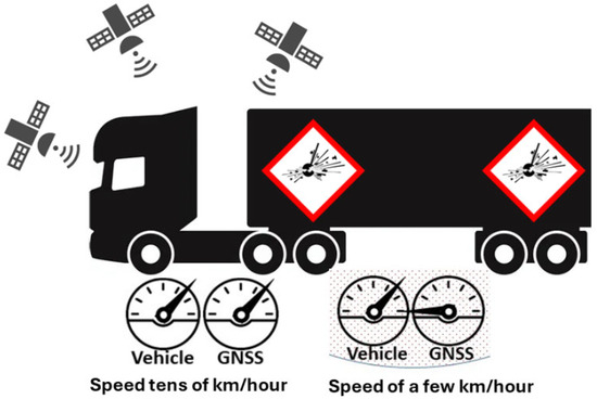
Figure 1.
Speed measurement by speedometers and GNSS navigator.
Speedometers, like any mechanical devices, produce errors. At low speeds, these errors are insignificant and are only 2–3 km/h. However, as the speed of the car increases, the degree of the inaccuracy of the speedometer readings also increases. For example, when driving at a speed of 90–100 km/h, the error can be 5–7 km/h, and at speeds of about 130 km/h it can reach 10–12 km/h.
2.1. GNSS Speed Measurement
GNSS speed measurement is largely based on the results of research in the field of GNSS cyber security [31,32,33,34,35,36,37,38,39,40,41], including the author’s research [42,43,44,45]. Suppose that:
—vehicle speed,
—frequency of vehicle coordinates measurements (1).
where is the number of measurements; are the coordinates of points , calculated by receivers; is the positioning error (the sum of deterministic and random errors); is the time synchronization error; is the error due to the geometrical arrangement of satellites; are ionospheric delays; are tropospheric delays; are ephemeris errors; are relativistic effects; are the instrumental errors and uncorrelated noise of the data transmission channel from satellites to receivers (uncorrelated noise); and is the positioning frequency.
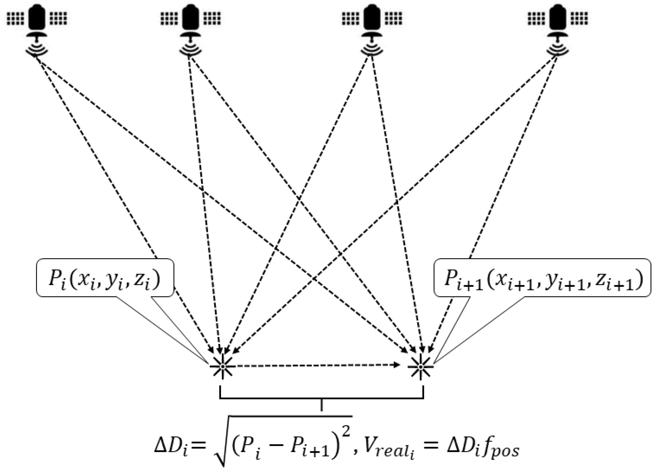
The GNSS speed measurement is based on the sequence (1) of vehicle positions shown in Figure 2.
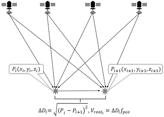
Figure 2.
GNSS speed measurement. If the distance between points Pi and Pi+1 is small (in the order of tens of centimeters) and the time interval between their positioning is also short (in the order of seconds), the speed of the vehicle can be determined with high accuracy.
Suppose that the distance between the points and is small (tens of centimeters) and the time between the positioning of the points and is also short (units of seconds). In this case, this can be written as (2)
where represents a fuzzy number with confidence interval boundaries (3)
where is the maximum value of .
According to the rules of blurred number arithmetic [46], this can be written as (4)
In this case, it is possible to define the distance between points and as (5):
It follows from Equation (6) that the largest value of the measurement error of the distance between points and can be written as (6)
2.2. GNSS Speed Measurement—Measuring Low-Speed Autonomous and Cargo Vehicles
The largest vehicle speed error can be defined as (7)
where ∆t is the sampling period of the measurements.
Therefore, considering error (7), the real speed of the vehicle must be set as (8)
where is the maximum permissible speed of a vehicle carrying highly dangerous loads.
2.3. The Definition of as the Maximum Value of
Suppose the vehicle is parked in its parking space. In this case, Equation (5) takes the following form (9):
This means that (10)
The sign here means that you need to compute the mean as an estimate of the expected value (11)
estimate the standard deviation of a random variable (12)
and to apply the 3-sigma rule, which states that for any random variable (in this case ) with a finite variance (in this case ), the probability that a random variable will deviate from its mathematical expectation by at least three standard deviations σ, no more than 1/9. That is (13)
Thus, the definition of as the maximum value of can be written as (14)
3. The Experiment
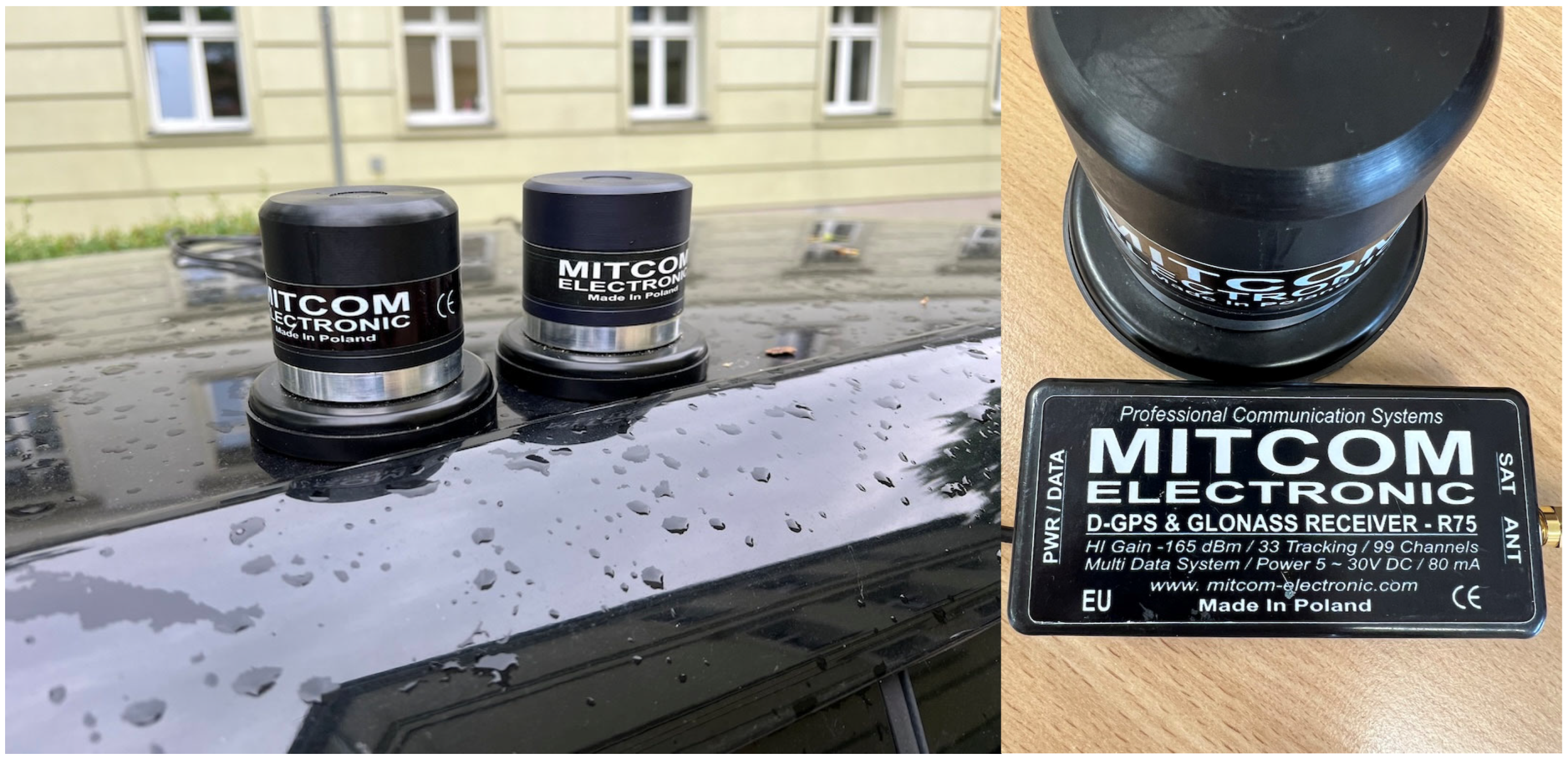
The experiment was carried out to determine the value in accordance with (14). 7383 measurements were performed. The experiment was conducted using two GPS-R75BT-5V receivers by Mitcom (Gdańsk, Poland) (Figure 3), maintaining the positioning accuracy parameters specified by the manufacturer (3D/2D accuracy ranging from 1 cm to 1.5 m, with an average accuracy of approximately 50 cm). The full specification is provided in source [47]. The experimental scenario involved simultaneously recording speed measurements from two GNSS receivers under controlled conditions to assess the accuracy and reliability of the proposed method. Each experiment lasted 2 h, during which over 7000 measurements were collected. To ensure the repeatability and consistency of the results, the experiment was repeated under various environmental and operational conditions.

Figure 3.
Mitcom GPS receivers mounted on the roof of a vehicle. The devices are placed close to each other and secured using magnetic bases. The experiment was conducted in outdoor conditions, as indicated by the raindrops on the car’s surface (left). A close-up view of one receiver along with its control module. The label on the module indicates its specifications, including D-GPS and GLONASS support, high-gain sensitivity of −165 dBm, 33 tracking channels, and 99 channels in total. It also operates with a multi-data system and requires a 5–30 V DC power supply at 80 mA (right).
The template for filling in the results of the experiment is given in Table 1 (for the case of the first 100 measurements). The table of the first 100 measurements is given in Appendix A.

Table 1.
Template of 100 latitude and longitude measurements series (N, E) 1.
The chart in Figure 4 shows changes in , which are differences in latitude measured in minutes for a series of 100 measurements. These changes oscillate between −0.0001 and 0.0001 min, indicating minor positional corrections as the vehicle moves. The figure illustrates irregular but repeatable jumps in value, which may indicate corrections by the GNSS system in response to dynamic environmental conditions affecting measurement accuracy. The oscillation patterns suggest that the vehicle was subjected to continuous, minor positional adjustments during the experiment.
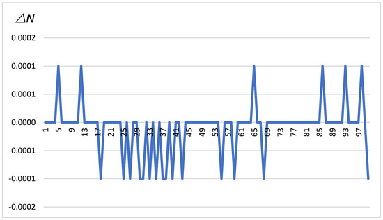
Figure 4.
∆N in minutes depending on the change number (on the x-axis).
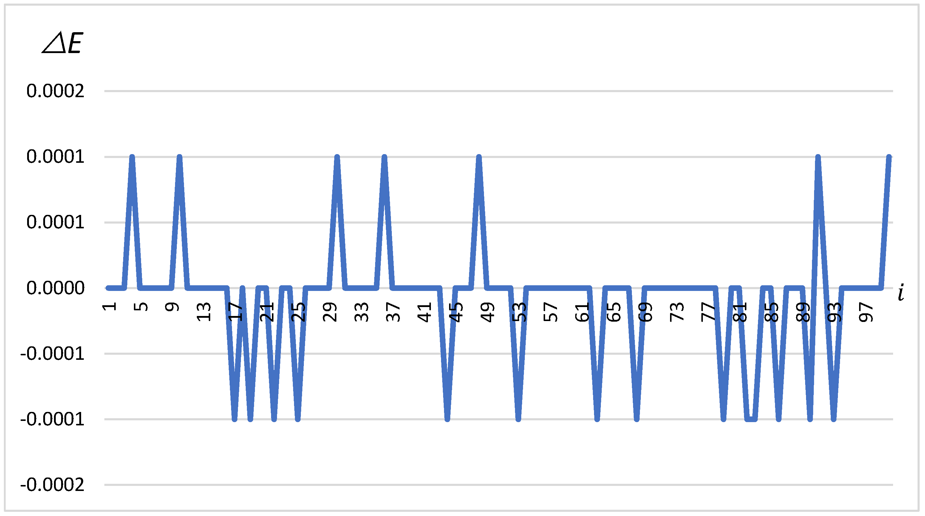
Similarly to the latitude, the changes in in Figure 5, which are differences in longitude, also oscillate between −0.0001 and 0.0001 min. The chart shows how frequently and to what extent the vehicle’s position was corrected in terms of longitude. Regular, sharp changes may indicate the high sensitivity of the navigation system to varying conditions, which is crucial for the precise navigation of a vehicle carrying dangerous materials.

Figure 5.
∆E in minutes depending on the change number (on the x-axis).
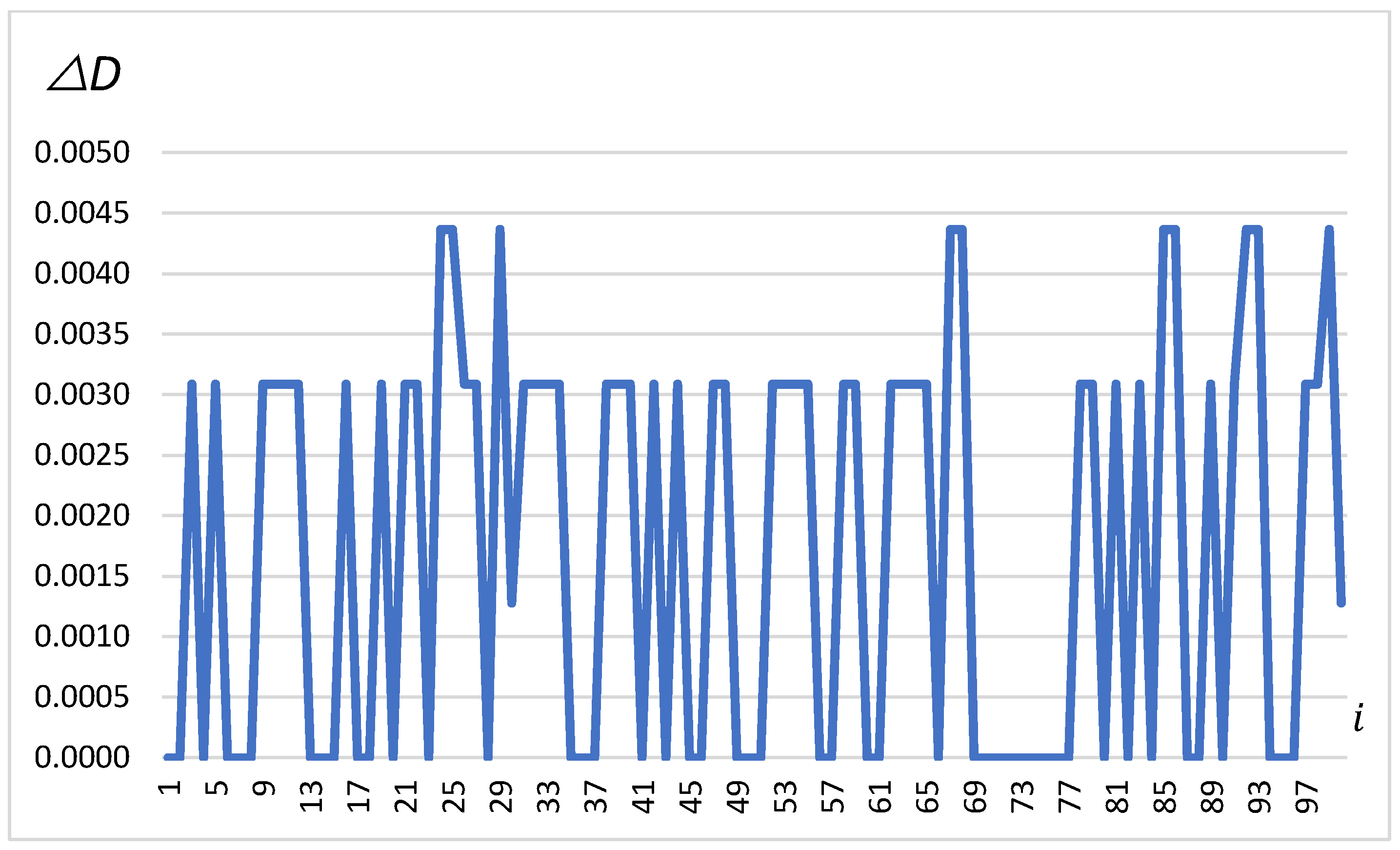
The third chart, in Figure 6, illustrates the changes in distance , calculated based on the previous differences and . These distances range between 0 and 0.0045 m, showing the variability and abruptness of the vehicle’s movement as recorded by the GNSS system. These jumps indicate how precisely the system measures the vehicle’s movement, which is essential for maintaining safety in the transport of highly dangerous loads.
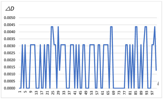
Figure 6.
∆D in meters depending on the change number (on the x-axis).
The analysis of the charts from the experiment on autonomous vehicles carrying dangerous loads provides valuable information about the accuracy and efficiency of the GNSS system in monitoring movement. Changes in and indicate the continuous correction of the vehicle’s autonomous positioning system, which is crucial when transporting materials that require high-precision navigation. Despite the small magnitude of changes, their regularity and frequency suggest that the navigation system is highly sensitive to any deviations from the planned route. Moreover, the changes in illustrate the abrupt nature of the vehicle’s movement, which can be useful for further refinement of the GNSS system algorithms to minimize risk during the transport of dangerous materials.
4. Relevance of Measurement
The high frequency of corrections and small deviations in GNSS data underline the importance of precision in designing transportation systems for special loads. This experiment confirms that even minor errors in data can lead to significant consequences, highlighting the need for continuous monitoring and analysis of navigational data. These results enhance our understanding of control and monitoring mechanisms in specialized autonomous transport, which is crucial for improving the safety and efficiency of transporting dangerous loads.
Assessment (15) is adequate only for a given area and for a given time ); that is, the assessment is of a local spatiotemporal nature (18):
To partially exclude the reference of the estimate over time, it is possible to repeat the described experiment; for example, every hour during the day and average the results obtained. In this case, the assessment is of a local spatial nature. In principle, such averaging can be performed for a certain region, for example, on the scale of a city or a group of cities. In this case, the assessment will be of a regional nature.
5. Conclusions
The study focused on road transport involving slow-moving vehicles carrying dangerous goods. Based on GNSS measurements, it was demonstrated that standard, widely available GNSS equipment can be effectively used to estimate low vehicle speeds with sufficient precision for safety monitoring purposes.
The proposed method responds to the need for enhanced tracking in transport scenarios where conventional speedometers may not provide accurate results, particularly at low speeds. Although the analysis was limited to a controlled environment, the collected data confirm the method’s consistency and operational feasibility.
Looking ahead, autonomous transport systems for hazardous cargo could significantly improve logistics safety. These systems can reduce human risk by enabling remote control and constant monitoring of key parameters such as location, speed, or cargo status. However, practical deployment will require high-reliability hardware, certified software, and strong regulatory frameworks—including cybersecurity and liability protocols. The collected data confirm the method’s consistency and operational feasibility.
The adoption of unmanned vehicle technologies also brings the following economic and operational advantages:
- Reduced fuel consumption due to smooth, optimized driving profiles;
- Lower personnel, maintenance, and operational costs;
- Time and resource savings through route optimization;
- Continuous operation without the need for driver rest breaks;
- A potential decrease in the number of road accidents.
Unmanned ground vehicles are particularly well suited for the transport of highly dangerous goods, offering the possibility to remove personnel from high-risk scenarios. Their precision in navigation and control makes them ideal for missions involving toxic substances, chemicals, or sensitive materials. While sharing some core technologies with autonomous passenger vehicles, the transport of goods presents additional challenges, such as increased weight and payload stability, which require dedicated solutions.
While the proposed GNSS-based method does not replace more advanced systems like LiDAR or INS, it offers a low-cost, reliable complement—especially in scenarios where the simplicity of implementation and accessibility of hardware are decisive factors. Future research will focus on testing the method under degraded signal conditions and comparing it directly with other sensor technologies.
The integration of GNSS-based systems into the broader context of autonomous logistics may offer a valuable contribution to improving safety in the transportation of dangerous goods.
Funding
This research received no external funding.
Data Availability Statement
The original contributions presented in this study are included in the article. Further inquiries can be directed to the corresponding author.
Conflicts of Interest
The author declares no conflict of interest.
Appendix A
| N | N (min) | E | E (min) | ∆N | ∆E | S (1–2) (m) |
|---|---|---|---|---|---|---|
| 5244.004 | 3164.004 | 1513.583 | 913.5825 | 0 | 0 | 0 |
| 5244.004 | 3164.004 | 1513.583 | 913.5825 | 0 | 0 | 0 |
| 5244.004 | 3164.004 | 1513.583 | 913.5825 | 0 | 0 | 0 |
| 5244.004 | 3164.004 | 1513.583 | 913.5825 | 0 | 1 × 10⁻⁴ | 0.003087 |
| 5244.004 | 3164.004 | 1513.582 | 913.5824 | 1 × 10⁻⁴ | 0 | 0.003087 |
| 5244.004 | 3164.004 | 1513.582 | 913.5824 | 0 | 0 | 0 |
| 5244.004 | 3164.004 | 1513.582 | 913.5824 | 0 | 0 | 0 |
| 5244.004 | 3164.004 | 1513.582 | 913.5824 | 0 | 0 | 0 |
| 5244.004 | 3164.004 | 1513.582 | 913.5824 | 0 | 0 | 0 |
| 5244.004 | 3164.004 | 1513.582 | 913.5824 | 0 | 0.0001 | 0.003087 |
| 5244.004 | 3164.004 | 1513.582 | 913.5823 | 0 | 0 | 0 |
| 5244.004 | 3164.004 | 1513.582 | 913.5823 | 1 × 10⁻⁴ | 0 | 0.003087 |
| 5244.004 | 3164.004 | 1513.582 | 913.5823 | 0 | 0 | 0 |
| 5244.004 | 3164.004 | 1513.582 | 913.5823 | 0 | 0 | 0 |
| 5244.004 | 3164.004 | 1513.582 | 913.5823 | 0 | 0 | 0 |
| 5244.004 | 3164.004 | 1513.582 | 913.5823 | 0 | 0 | 0 |
| 5244.004 | 3164.004 | 1513.582 | 913.5823 | 0 | −0.0001 | 0.003087 |
| 5244.004 | 3164.004 | 1513.582 | 913.5824 | −1 × 10⁻⁴ | 0 | 0.003087 |
| 5244.004 | 3164.004 | 1513.582 | 913.5824 | 0 | −1 × 10⁻⁴ | 0.003087 |
| 5244.004 | 3164.004 | 1513.583 | 913.5825 | 0 | 0 | 0 |
| 5244.004 | 3164.004 | 1513.583 | 913.5825 | 0 | 0 | 0 |
| 5244.004 | 3164.004 | 1513.583 | 913.5825 | 0 | −1 × 10⁻⁴ | 0.003087 |
| 5244.004 | 3164.004 | 1513.583 | 913.5826 | 0 | 0 | 0 |
| 5244.004 | 3164.004 | 1513.583 | 913.5826 | 0 | 0 | 0 |
| 5244.004 | 3164.004 | 1513.583 | 913.5826 | −1 × 10⁻⁴ | −0.0001 | 0.004366 |
| 5244.004 | 3164.004 | 1513.583 | 913.5827 | 0 | 0 | 0 |
| 5244.004 | 3164.004 | 1513.583 | 913.5827 | −0.0001 | 0 | 0.003087 |
| 5244.004 | 3164.004 | 1513.583 | 913.5827 | 0 | 0 | 0 |
| 5244.004 | 3164.004 | 1513.583 | 913.5827 | 0 | 0 | 0 |
| 5244.004 | 3164.004 | 1513.583 | 913.5827 | −0.0001 | 0.0001 | 0.004366 |
| 5244.004 | 3164.004 | 1513.583 | 913.5826 | −1 × 10⁻⁴ | 0 | 0.003087 |
| 5244.003 | 3164.003 | 1513.583 | 913.5826 | 0 | 0 | 0 |
| 5244.003 | 3164.003 | 1513.583 | 913.5826 | −1 × 10⁻⁴ | 0 | 0.003087 |
| 5244.003 | 3164.003 | 1513.583 | 913.5826 | 0 | 0 | 0 |
| 5244.003 | 3164.003 | 1513.583 | 913.5826 | −0.0001 | 0 | 0.003087 |
| 5244.003 | 3164.003 | 1513.583 | 913.5826 | 0 | 1 × 10⁻⁴ | 0.003087 |
| 5244.003 | 3164.003 | 1513.583 | 913.5825 | −1 × 10⁻⁴ | 0 | 0.003087 |
| 5244.003 | 3164.003 | 1513.583 | 913.5825 | −1 × 10⁻⁴ | 0 | 0.003087 |
| 5244.003 | 3164.003 | 1513.583 | 913.5825 | 0 | 0 | 0 |
| 5244.003 | 3164.003 | 1513.583 | 913.5825 | −0.0001 | 0 | 0.003087 |
| 5244.003 | 3164.003 | 1513.583 | 913.5825 | 0 | 0 | 0 |
| 5244.003 | 3164.003 | 1513.583 | 913.5825 | 0 | 0 | 0 |
| 5244.003 | 3164.003 | 1513.583 | 913.5825 | −1 × 10⁻⁴ | 0 | 0.003087 |
| 5244.003 | 3164.003 | 1513.583 | 913.5825 | 0 | −1 × 10⁻⁴ | 0.003087 |
| 5244.003 | 3164.003 | 1513.583 | 913.5826 | 0 | 0 | 0 |
| 5244.003 | 3164.003 | 1513.583 | 913.5826 | 0 | 0 | 0 |
| 5244.003 | 3164.003 | 1513.583 | 913.5826 | 0 | 0 | 0 |
| 5244.003 | 3164.003 | 1513.583 | 913.5826 | 0 | 1 × 10⁻⁴ | 0.003087 |
| 5244.003 | 3164.003 | 1513.583 | 913.5825 | 0 | 0 | 0 |
| 5244.003 | 3164.003 | 1513.583 | 913.5825 | 0 | 0 | 0 |
| 5244.003 | 3164.003 | 1513.583 | 913.5825 | 0 | 0 | 0 |
| 5244.003 | 3164.003 | 1513.583 | 913.5825 | 0 | 0 | 0 |
| 5244.003 | 3164.003 | 1513.583 | 913.5825 | 0 | −1 × 10⁻⁴ | 0.003087 |
| 5244.003 | 3164.003 | 1513.583 | 913.5826 | 0 | 0 | 0 |
| 5244.003 | 3164.003 | 1513.583 | 913.5826 | −1 × 10⁻⁴ | 0 | 0.003087 |
| 5244.003 | 3164.003 | 1513.583 | 913.5826 | 0 | 0 | 0 |
| 5244.003 | 3164.003 | 1513.583 | 913.5826 | 0 | 0 | 0 |
| 5244.003 | 3164.003 | 1513.583 | 913.5826 | 0 | 0 | 0 |
| 5244.003 | 3164.003 | 1513.583 | 913.5826 | −0.0001 | 0 | 0.003087 |
| 5244.003 | 3164.003 | 1513.583 | 913.5826 | 0 | 0 | 0 |
| 5244.003 | 3164.003 | 1513.583 | 913.5826 | 0 | 0 | 0 |
| 5244.003 | 3164.003 | 1513.583 | 913.5826 | 0 | 0 | 0 |
| 5244.003 | 3164.003 | 1513.583 | 913.5826 | 0 | −0.0001 | 0.003087 |
| 5244.003 | 3164.003 | 1513.583 | 913.5827 | 0 | 0 | 0 |
| 5244.003 | 3164.003 | 1513.583 | 913.5827 | 0.0001 | 0 | 0.003087 |
| 5244.003 | 3164.003 | 1513.583 | 913.5827 | 0 | 0 | 0 |
| 5244.003 | 3164.003 | 1513.583 | 913.5827 | 0 | 0 | 0 |
| 5244.003 | 3164.003 | 1513.583 | 913.5827 | −0.0001 | −0.0001 | 0.004366 |
| 5244.003 | 3164.003 | 1513.583 | 913.5828 | 0 | 0 | 0 |
| 5244.003 | 3164.003 | 1513.583 | 913.5828 | 0 | 0 | 0 |
| 5244.003 | 3164.003 | 1513.583 | 913.5828 | 0 | 0 | 0 |
| 5244.003 | 3164.003 | 1513.583 | 913.5828 | 0 | 0 | 0 |
| 5244.003 | 3164.003 | 1513.583 | 913.5828 | 0 | 0 | 0 |
| 5244.003 | 3164.003 | 1513.583 | 913.5828 | 0 | 0 | 0 |
| 5244.003 | 3164.003 | 1513.583 | 913.5828 | 0 | 0 | 0 |
| 5244.003 | 3164.003 | 1513.583 | 913.5828 | 0 | 0 | 0 |
| 5244.003 | 3164.003 | 1513.583 | 913.5828 | 0 | 0 | 0 |
| 5244.003 | 3164.003 | 1513.583 | 913.5828 | 0 | 0 | 0 |
| 5244.003 | 3164.003 | 1513.583 | 913.5828 | 0 | −0.0001 | 0.003087 |
| 5244.003 | 3164.003 | 1513.583 | 913.5829 | 0 | 0 | 0 |
| 5244.003 | 3164.003 | 1513.583 | 913.5829 | 0 | 0 | 0 |
| 5244.003 | 3164.003 | 1513.583 | 913.5829 | 0 | −1 × 10⁻⁴ | 0.003087 |
| 5244.003 | 3164.003 | 1513.583 | 913.583 | 0 | −1 × 10⁻⁴ | 0.003087 |
| 5244.003 | 3164.003 | 1513.583 | 913.5831 | 0 | 0 | 0 |
| 5244.003 | 3164.003 | 1513.583 | 913.5831 | 0 | 0 | 0 |
| 5244.003 | 3164.003 | 1513.583 | 913.5831 | 0.0001 | −0.0001 | 0.004366 |
| 5244.003 | 3164.003 | 1513.583 | 913.5832 | 0 | 0 | 0 |
| 5244.003 | 3164.003 | 1513.583 | 913.5832 | 0 | 0 | 0 |
| 5244.003 | 3164.003 | 1513.583 | 913.5832 | 0 | 0 | 0 |
| 5244.003 | 3164.003 | 1513.583 | 913.5832 | 0 | −0.0001 | 0.003087 |
| 5244.003 | 3164.003 | 1513.583 | 913.5833 | 0 | 0.0001 | 0.003087 |
| 5244.003 | 3164.003 | 1513.583 | 913.5832 | 0 | 0 | 0 |
| 5244.003 | 3164.003 | 1513.583 | 913.5832 | 1 × 10⁻⁴ | −0.0001 | 0.004366 |
| 5244.003 | 3164.003 | 1513.583 | 913.5833 | 0 | 0 | 0 |
| 5244.003 | 3164.003 | 1513.583 | 913.5833 | 0 | 0 | 0 |
| 5244.003 | 3164.003 | 1513.583 | 913.5833 | 0 | 0 | 0 |
| 5244.003 | 3164.003 | 1513.583 | 913.5833 | 0 | 0 | 0 |
| 5244.003 | 3164.003 | 1513.583 | 913.5833 | 1 × 10⁻⁴ | 0 | 0.003087 |
| 5244.003 | 3164.003 | 1513.583 | 913.5833 | 0 | 0 | 0 |
| 5244.003 | 3164.003 | 1513.583 | 913.5833 | −1 × 10⁻⁴ | 0.0001 | 0.004366 |
References
- Transport of Dangerous Goods. Available online: https://unece.org/DAM/trans/danger/publi/unrec/rev17/English/Rev17_Volume1.pdf (accessed on 1 November 2024).
- The 9 Classes of Dangerous Goods. Available online: https://www.sainthelena.gov.sh/wp-content/uploads/2012/08/The-Nine-Classes-of-Dangerous-Goods.pdf (accessed on 1 November 2024).
- Appendix on Dangerous Goods. Available online: https://www.icao.int/safety/DangerousGoods/Working%20Group%20of%20the%20Whole/WP.50.AppB.pdf (accessed on 1 November 2024).
- Transportation of Dangerous Goods Regulations. Available online: https://tc.canada.ca/sites/default/files/migrated/single_pdf_sor_2019_101___archived.pdf (accessed on 1 November 2024).
- Greatrix, G. Vehicle Speed Measurement and Law Enforcement. Meas. Control 2011, 44, 249–251. [Google Scholar] [CrossRef]
- Pourzeynali, S.; Zhu, X.; Ghari Zadeh, A.; Rashidi, M.; Samali, B. Comprehensive Study of Moving Load Identification on Bridge Structures Using the Explicit Form of Newmark-β Method: Numerical and Experimental Studies. Remote Sens. 2021, 13, 2291. [Google Scholar] [CrossRef]
- Socha, A.; Izydorczyk, J. Strain Gauge Calibration for High Speed Weight-in-Motion Station. Sensors 2024, 24, 4845. [Google Scholar] [CrossRef] [PubMed]
- Oubrich, L.; Ouassaid, M.; Maaroufi, M. Dynamic loads, source of errors of high speed weigh in motion systems. In Proceedings of the 2017 14th International Multi-Conference on Systems, Signals & Devices (SSD), Marrakech, Morocco, 28–31 March 2017; pp. 354–359. [Google Scholar] [CrossRef]
- Paszek, K.; Grzechca, D. Using the LSTM Neural Network and the UWB Positioning System to Using the LSTM Neural Network and the UWB Positioning System to Predict the Position of Low and High Speed Moving Objects. Sensors 2023, 23, 8270. [Google Scholar] [CrossRef] [PubMed]
- Fornasa, M.; Zingirian, N.; Maresca, M. Extensive GPRS Latency Characterization in Uplink Packet Transmission from Moving Vehicles. In Proceedings of the VTC Spring 2008—IEEE Vehicular Technology Conference, Marina Bay, Singapore, 11–14 May 2008; pp. 2562–2566. [Google Scholar] [CrossRef]
- Malviya, A.; Kala, R. Risk Modeling of the Overtaking Behavior in the Indian Traffic. In Proceedings of the 2022 IEEE 25th International Conference on Intelligent Transportation Systems (ITSC), Macau, China, 8–12 October 2022; pp. 2882–2887. [Google Scholar] [CrossRef]
- Taubert, S.; Wierzejski, A. Influence the structure of the road surface on the measurement of distance and speed using optical head. J. KONES Powertrain Transp. 2015, 20, 465–469. [Google Scholar] [CrossRef]
- Liang, J.; Tian, Q.; Feng, J.; Pi, D. A Polytopic Model-Based Robust Predictive Control Scheme for Path Tracking of Autonomous Vehicles. IEEE Trans. Intell. Veh. 2024, 9, 3928–3939. [Google Scholar] [CrossRef]
- Lienert, P. Self-Driving Cars Could Generate Billions in Revenue: U.S. Study//Reuters. 5 March 2015. Available online: https://www.reuters.com/article/us-usa-autosautonomous/self-driving-cars-could-generate-billionsin-revenue-u-s-study-idUSKBN0M10UF20150305 (accessed on 1 November 2024).
- Borkowski, P. Inference engine in an intelligent ship course-keeping system. Comput. Intell. Neurosci. 2017, 2017, 2561383. [Google Scholar] [CrossRef] [PubMed]
- Borkowski, P.; Zwierzewicz, Z. Ship course-keeping algorithm based on knowledge base. Intell. Autom. Soft Comput. 2011, 17, 149–163. [Google Scholar] [CrossRef]
- Self-Driving Vehicles in Logistics. A DHL Perspective on Implications and Use Cases for the Logistics Industry. DHL Trend Research. 2014. 39p. Available online: https://www.dhl.com/discover/content/dam/dhl/downloads/interim/full/dhl-self-driving-vehicles.pdf (accessed on 1 November 2024).
- Autonomous vehicles. Handing Over Control: Opportunities and Risks for Insurance. Lloyd’s. 2014. 27p. Available online: https://assets.lloyds.com/assets/pdf-autonomous-vehicles/1/pdf-autonomous-vehicles.pdf (accessed on 1 November 2024).
- Autonomous Vehicles: Navigating the Legal and Regulatory Issues of a Driverless World. Available online: https://mcca.com/wp-content/uploads/2018/04/Autonomous-Vehicles.pdf (accessed on 1 November 2024).
- Torc. Trucking: Trucks Keep Our World Moving. Available online: https://torc.ai/partnerships (accessed on 1 November 2024).
- Johnson, P. How Ford’s BlueCruise Hands-Free Tech Is Keeping Drivers Safe and Even Changing Lives. Electrek, 7 February 2023. [Google Scholar]
- Teamsters, Tech Firms Tangle Over Self-Driving Trucks Bill. Available online: https://news.bloomberglaw.com (accessed on 1 November 2024).
- Liang, Y.; Zheng, Z. MARL-OT: Multi-Agent Reinforcement Learning for Online Fuzz Testing of Autonomous Driving Systems. arXiv 2025, arXiv:2501.14451. [Google Scholar] [CrossRef]
- Nweje, I.E.; Onuma, A. Autonomous Vehicles in the Logistics Supply Chain: A Study of Regulatory, Safety, and Operational Challenges. Adv. Transp. Res. 2025, 1, 1239908. [Google Scholar] [CrossRef]
- Milenković, M.; Sumpor, D.; Tokić, S. Legal and Safety Aspects of the Application of Automated and Autonomous Vehicles in the Republic of Croatia. World Electr. Veh. J. 2025, 16, 34. [Google Scholar] [CrossRef]
- Jamuna, P.; Kumar, K.K.; Murugesan, A.; Karthikeyan, G.; Dineshkumar, S.; Sangeetha, M. Intelligent Automation in Long Vehicles through LDR Sensor Technology for Accident Prevention. In Proceedings of the 2024 International Conference on Communication, Computing and Internet of Things (IC3IoT), Chennai, India, 17–18 April 2024; pp. 1–6. [Google Scholar] [CrossRef]
- Liang, J.; Feng, J.; Lu, Y.; Yin, G.; Zhuang, W.; Mao, X. A Direct Yaw Moment Control Framework through Robust T–S Fuzzy Approach Considering Vehicle Stability Margin. IEEE/ASME Trans. Mechatron. 2024, 29, 166–178. [Google Scholar] [CrossRef]
- Shi, Y.; Dong, H.; He, C.R.; Chen, Y.; Song, Z. Mixed Vehicle Platoon Forming: A Multi-Agent Reinforcement Learning Approach. IEEE Internet Things J. 2025. [Google Scholar] [CrossRef]
- Vehicle Speed Measurement Technique Using Various Speed Detection Instrumentation. Available online: https://www.researchgate.net/publication/261238039_Vehicle_speed_measurement_technique_using_various_speed_detection_instrumentation (accessed on 1 November 2024).
- Psiaki, M.L.; O’Hanlon, B.W.; Powell, S.P.; Bhatti, J.A.; Wesson, K.D.; Humphreys, T.E.; Schofield, A. GNSS Spoofing Detection using Two-Antenna Differential Carrier Phase. In Proceedings of the 27th international technical meeting of the satellite division of the Institute of Navigation (ION GNSS+ 2014), Tampa, FL, USA, 8–12 September 2014. [Google Scholar]
- Zalewski, P. Real-time GNSS spoofing detection in maritime code receivers. Sci. J. Marit. Univ. Szczec. 2014, 38, 118–124. [Google Scholar]
- Humphreys, T.E. Detection Strategy for Cryptographic GNSS Anti-Spoofing. IEEE Trans. Aerosp. Electron. Syst. 2013, 49, 1073–1090. [Google Scholar] [CrossRef]
- Levin, P.; De Lorenzo, D.S.; Enge, P.K.; Lo, S.C. Authenticating a Signal Based on an Unknown Component Thereof. U.S. Patent No. 7,969,354 B2, 28 June 2011. [Google Scholar]
- Li, Z.; Gebre-Egziabher, D. Performance Analysis of a Civilian GPS Position Authentication System. Navigation 2013, 60, 246–265. [Google Scholar] [CrossRef]
- Caparra, G.; Ceccato, S.; Laurenti, N.; Cramer, J. Feasibility and Limitations of Self-Spoofing Attacks on GNSS Signals with Message Authentication. In Proceedings of the 30th International Technical Meeting of the Satellite Division of The Institute of Navigation (ION GNSS+ 2017), Portland, Oregon, 25–29 September 2017; pp. 3968–3984. [Google Scholar]
- Psiaki, M.L.; Powell, S.P.; O’Hanlon, B.W. GNSS Spoofing Detection Using High-Frequency Antenna Motion and Carrier-Phase Data. In Proceedings of the 26th International Technical Meeting of the Satellite Division of the Institute of Navigation (ION GNSS+ 2013), Nashville, TN, USA, 16–20 September 2013; pp. 2949–2991. [Google Scholar]
- Swaszek, P.F.; Hartnett, R.J. A Multiple COTS Receiver GNSS Spoof Detector—Extensions. In Proceedings of the International Technical Meeting of the ION, San Diego, CA, USA, 8–12 September 2014; pp. 316–326. [Google Scholar]
- Trinkle, M.; Zhang, Z.; Li, H.; Dimitrovski, A. GPS Anti-Spoofing Techniques for Smart Grid Applications. In Proceedings of the 25th International Technical Meeting of the Satellite Division of The Institute of Navigation (ION GNSS 2012), Nashville, TN, USA, 17–21 September 2012; pp. 1270–1278. [Google Scholar]
- Hwang, P.Y.; McGraw, G.A. Receiver Autonomous Signal Authentication (RASA) Based on Clock Stability Analysis. In Proceedings of the 2014 IEEE/ION Position, Location and Navigation Symposium-PLANS 2014, Monterey, CA, USA, 5–8 May 2014; pp. 270–281. [Google Scholar]
- Pini, M.; Fantino, M.; Cavaleri, A.; Ugazio, S.; Lo Presti, L. Signal Quality Monitoring Applied to Spoofing Detection. In Proceedings of the 24th International Technical Meeting of The Satellite Division of the Institute of Navigation (ION GNSS 2011), Portland, OR, USA, 20–23 September 2011; pp. 1888–1896. [Google Scholar]
- Yuan, D.; Li, H.; Lu, M.A. Method for GNSS Spoofing Detection Based on Sequential Probability Ratio Test. In Proceedings of the 2014 IEEE/ION Position, Location and Navigation Symposium-PLANS 2014, Monterey, CA, USA, 5–8 May 2014; pp. 351–358. [Google Scholar]
- Lemieszewski, Ł.; Radomska-Zalas, A.; Perec, A.; Dobryakova, L.; Ochin, E. The Spoofing Detection of Dynamic Underwater Positioning Systems (DUPS) Based on Vehicles Retrofitted with Acoustic Speakers. Electronics 2021, 10, 2089. [Google Scholar] [CrossRef]
- Ochin, E.; Lemieszewski, Ł. Układ do Wykrywania Elektronicznego Ataku Typu Spoofing Sygnału Globalnego Systemu Nawigacji Satelitarnej GNSS. 2019; Application no. 432296. pp. 61–62. Available online: https://uprp.gov.pl/sites/default/files/bup/2021/Wynalazki%20i%20wzory%20u%C5%BCytkowe/06_12-13/13//bup13_2021.pdf (accessed on 1 November 2024).
- Lemieszewski, Ł.; Radomska-Zalas, A.; Perec, A.; Dobryakova, L.; Ochin, E. GNSS and LNSS Positioning of Unmanned Transport Systems: The Brief Classification of Terrorist Attacks on USVs and UUVs. Electronics 2021, 10, 401. [Google Scholar] [CrossRef]
- Dobryakova, L.; Lemeszewski, Ł.; Ochin, E. GNSS Spoofing Detection Using Static or Rotating Single-Antenna of a Static or Moving Victim. IEEE Access 2018, 6, 79074–79081. [Google Scholar] [CrossRef]
- Stefanini, L.; Sorini, L.; Guerra, M. Fuzzy Numbers and Fuzzy Arithmetic. In Handbook of Granular Computing; Pedrycz, W., Skowron, A., Kreinovich, V., Eds.; John Wiley & Sons, Ltd.: Oxford, UK, 2008; Chapter 12; pp. 249–283. [Google Scholar]
- Mitcom Electronic. GPS R75BT A-GPS HV60—Professional Precision D-GPS/GLONASS Receiver with Bluetooth and Shock-Resistant Fixed-Mount Antenna for Agriculture, Transport, and Navigation. Available online: https://mitcom-electronic.shoplo.com/gps-r75bt-agps-hv60-profesjonalny-precyzyjny-odbiornik-d-gps-glonass-z-funkcja-bluetooth-specjalistyczna-udar-odporna-antena-do-montazu-stalego-rolnictwo-transport-nawigacja-kopia (accessed on 21 March 2025).


Disclaimer/Publisher’s Note: The statements, opinions and data contained in all publications are solely those of the individual author(s) and contributor(s) and not of MDPI and/or the editor(s). MDPI and/or the editor(s) disclaim responsibility for any injury to people or property resulting from any ideas, methods, instructions or products referred to in the content. |
© 2025 by the author. Licensee MDPI, Basel, Switzerland. This article is an open access article distributed under the terms and conditions of the Creative Commons Attribution (CC BY) license (https://creativecommons.org/licenses/by/4.0/).