Abstract
Industrial control systems (ICSs) are a critical component of key infrastructure. However, as ICSs transition from isolated systems to modern networked environments, they face increasing security risks. Traditional anomaly detection methods struggle with complex ICS traffic due to their failure to fully utilize both low-frequency and high-frequency traffic information, and their poor performance in heterogeneous and non-stationary data environments. Moreover, fixed threshold methods lack adaptability and fail to respond in real time to dynamic changes in traffic, resulting in false positives and false negatives. To address these issues, this paper proposes a deep learning-based traffic anomaly detection algorithm. The algorithm employs the Hilbert–Huang Transform (HHT) to decompose traffic features and extract multi-frequency information. By integrating feature and temporal attention mechanisms, it enhances modeling capabilities and improves prediction accuracy. Additionally, the deep probabilistic estimation approach dynamically adjusts confidence intervals, enabling synchronized prediction and detection, which significantly enhances both real-time performance and accuracy. Experimental results demonstrate that our method outperforms existing baseline models in both prediction and anomaly detection performance on a real-world industrial control traffic dataset collected from an oilfield in China. The dataset consists of approximately 260,000 records covering Transmission Control Protocol/User Datagram Protocol (TCP/UDP) traffic between Remote Terminal Unit (RTU), Programmable Logic Controller (PLC), and Supervisory Control and Data Acquisition (SCADA) devices. This study has practical implications for improving the cybersecurity of ICSs and provides a theoretical foundation for the efficient management of industrial control networks.
1. Introduction
Industrial control systems (ICSs) are widely employed in critical infrastructure sectors such as power generation, water treatment, oil and gas, and chemical processing. Their stability and security are directly tied to public health, safety, and environmental protection [1,2]. With the advancement of network technologies, ICSs have gradually transitioned from traditional isolated systems to modern networked systems based on standardized protocols and devices. This evolution enables ICSs to interact more flexibly with other information systems but also introduces heightened security risks [3]. In recent years, ICSs have become frequent targets of cyberattacks, posing significant threats to the normal operation of industrial systems [4]. For instance, in 2010, the Stuxnet worm infected the programmable logic controllers (PLCs) of Iran’s nuclear facilities, disrupting the normal operation of centrifuges [5]. In 2015 and 2016, Ukraine’s power grid was targeted by hackers using the malware BlackEnergy and Industroyer, resulting in widespread power outages [6]. In 2017, the Triton malware attacked the safety instrumented system (SIS) of a Saudi petrochemical plant, aiming to cause equipment malfunctions [7]. These incidents underscore the increasing targeting of ICSs by cyber adversaries, highlighting the increasingly critical and urgent nature of ICS security challenges [8,9].
The security of industrial control system (ICS) networks has always been a focal point for researchers both domestically and internationally, with anomaly detection systems becoming a key area of research in this field. In recent years, anomaly detection methods based on multi-physical quantity fusion have been proven to effectively enhance the accuracy of industrial equipment health status assessment [10]. Additionally, systematic studies on communication protocol security, such as fuzz testing frameworks, have provided new perspectives for discovering vulnerabilities in ICS networks [11]. However, traditional anomaly detection methods have typically focused on static analysis or offline processing [12], which fail to meet the real-time monitoring and rapid response needs of industrial control systems. In ICS networks, traffic data typically exhibit significant temporal dependencies. Leveraging these dependencies within time series can effectively detect anomalies in traffic patterns [13]. Based on these characteristics and the need for real-time anomaly detection in ICS networks, real-time traffic prediction has emerged as a promising research direction. This approach allows for the continuous monitoring and prediction of traffic patterns in ICS networks, providing robust support for anomaly detection [14]. However, this research direction faces several challenges. In ICS networks, the diverse operating modes of different industrial control devices result in traffic data that are heterogeneous, nonlinear, and highly noisy [15]. Data from various devices often differ significantly in terms of scale, frequency, and sampling methods, complicating real-time traffic analysis [16,17]. Additionally, ICS traffic data are highly dynamic, fluctuating with changes in production tasks. These dynamics make anomaly detection methods based on traffic prediction increasingly difficult [18]. The key challenge lies in accurately extracting valuable information in real time and identifying anomalies within such a heterogeneous and dynamic ICS environment. There is currently limited research on real-time anomaly detection methods based on traffic prediction in industrial control network environments. Moreover, existing studies suffer from the following issues:
- Although industrial control network traffic is generally stable, short-term fluctuations can occur under certain circumstances. Both low-frequency stable trends and high-frequency short-term variations may contain critical traffic pattern information. However, existing research has often failed to fully explore and utilize the information embedded in both low- and high-frequency traffic data.
- Traffic data in industrial control systems exhibit strong temporal dependencies, characterized by complex short-term variations that significantly change based on work cycles, operational states, or device conditions, thereby increasing the complexity of traffic patterns. Additionally, traffic data exhibit long-term dependencies, requiring continuous observation of historical data to capture potential anomalies. However, existing detection methods struggle to effectively model such complex temporal dependencies and long-term patterns. In particular, they often fail to handle dynamic changes and long-term trends, leading to increased false positives or false negatives, which in turn reduces anomaly detection accuracy.
- Traditional residual-based evaluation methods rely on fixed thresholds to determine anomalies, but these thresholds are typically set based on empirical rules and lack adaptive capabilities. Under different operational environments, load levels, or system states, the normal fluctuation range of traffic may vary. Fixed-threshold methods thus struggle to accommodate the diversity and non-stationarity of traffic data, limiting their effectiveness in real-world applications.
To address the aforementioned issues and enhance the security of industrial control networks, this paper proposes a deep learning-based real-time monitoring algorithm for traffic anomaly detection in ICSs. The proposed method employs the Hilbert–Huang Transform(HHT) to decompose time series data, effectively capturing temporal characteristics of network traffic. Additionally, a cross-frequency and cross-period attention module is introduced to model time series dependencies. Finally, a deep probabilistic estimation model is used in place of traditional point estimation strategies, improving the dynamic adaptability of anomaly detection.
The main contributions of this paper are summarized as follows:
- We design a novel signal decoupling module that utilizes Empirical Mode Decomposition (EMD) to decompose raw traffic signals into feature components of different frequencies, enhancing the capability of extracting time series features.
- We propose a cross-frequency and cross-period attention mechanism that integrates a feature-attentive encoder with a time-attentive decoder, improving the model’s ability to capture multi-scale temporal dependencies and enhancing the accuracy of traffic prediction.
- We introduce an anomaly detection method based on deep probabilistic estimation, enabling the model to dynamically adapt to variations in traffic distributions across different ICS environments. This allows for dynamic adjustments in prediction outcomes, effectively handling diverse and non-stationary traffic data, thereby improving detection robustness and accuracy.
The remainder of this paper is organized as follows. Section 2 reviews related research. The details of the proposed model are presented in Section 3. In Section 4, we evaluate the performance of the proposed algorithm on real-world ICS traffic data. A performance analysis and discussion of the results are provided in the final section.
2. Related Work
Numerous anomaly behavior detection methods have been proposed to date. Early anomaly detection systems often employed statistical models, which primarily relied on constructing generative models capable of accurately representing the distribution characteristics of a given dataset. During detection, the model evaluates the probability value of each data point and identifies those located in low-probability regions or significantly deviating from the main distribution as anomalies. Nakamura et al. proposed an anomaly detection algorithm called MERLIN, which effectively detects discordant points of varying lengths by sliding windows through time series and combining the distances of subsequences [19]. Waskita et al. proposed an intrusion detection method based on modeling the statistical characteristics of network traffic, which effectively identifies normal and threat traffic through exhaustive search decision systems [20]. Moustafa et al. introduced a statistical anomaly detection technique based on the Dirichlet Mixture Model (DMM), which, by integrating the interquartile range boundaries, can distinguish legitimate traffic from attack vectors [21]. Andrysiak et al. presented a hybrid statistical model based on ARIMA-GARCH for detecting attack anomalies in network traffic. This method improves detection accuracy and efficiency through time series standardization, heteroscedasticity testing, and parameter optimization [22]. While statistical methods can achieve anomaly detection to some extent, they often depend on predefined probability distributions and simple thresholds, making it challenging to adapt effectively to complex and dynamically changing traffic patterns, leading to increased false positives and false negatives. With the rapid development of machine learning and deep learning, more researchers are turning to intelligent methods for anomaly detection research. These approaches can be broadly divided into supervised and unsupervised techniques. Yulianto et al. proposed an improved intrusion detection system based on AdaBoost, which addresses the data imbalance problem through the Synthetic Minority Oversampling Technique (SMOTE) and improves system performance by employing Principal Component Analysis (PCA) and Ensemble Feature Selection (EFS) to extract important features [23]. Farooq et al. proposed a multi-layer classification strategy to address the inability of the signature-based intrusion detection system SNORT to automatically recognize new attack signatures and detect multi-stage attacks. This method uses decision trees and fuzzy logic to automatically update SNORT signatures for detecting new attacks [24]. Song et al. introduced a novel intrusion detection method that combines Long Short-Term Memory (LSTM) and eXtreme Gradient Boosting (XGBoost) models to enhance intrusion detection effectiveness in smart grids by leveraging the accuracy of these two models [25]. Supervised learning requires labeled training data for normal and attack scenarios; however, labeled data for industrial control system (ICS) network attacks can be challenging to obtain [26], and such data often do not include unknown attack categories. Subsequently, unsupervised learning methods for anomaly detection have been proven effective. These methods do not require labeled anomalous data during the training phase [27]. They achieve anomaly detection by constructing deep neural networks to learn the complex feature relationships of multidimensional time series data, either by predicting future time series or reconstructing normal time series patterns, enabling the effective identification and detection of anomalies that deviate from normal patterns. Zeng et al. proposed an improved HTM algorithm model for anomaly detection in industrial multivariate time series data. The model encodes each dimension of the multivariate data separately, processes the encoded results using multiple spatial poolers in parallel, and combines the spatial pooler outputs in a temporal memory layer to predict future data, thereby enhancing anomaly detection performance for multivariate time series [28]. Chen et al. proposed an unsupervised model, SOM-DAGMM, that integrates Self-Organizing Maps (SOMs) with a Deep Autoencoding Gaussian Mixture Model (DAGMM) to address DAGMM’s limitations in preserving input topology. A SOM provides the topological preservation of features, and multi-scale topology further improves detection performance [29]. Niu et al. introduced a time series anomaly detection method based on LSTM and VAE-GAN, which jointly trains the encoder, generator, and discriminator to fully exploit their mapping and discriminative capabilities. During the anomaly detection phase, anomalies are identified based on reconstruction differences and discrimination results [30]. Boppana et al. proposed an unsupervised model, GAN-AE, that combines Generative Adversarial Networks (GANs) and Autoencoders (AEs) for detecting unknown intrusions in MQTT IoT applications and achieved promising results [31]. Zhao et al. presented a self-supervised framework that captures the complex dependencies of multivariate time series across temporal and feature dimensions using parallel graph attention layers. This method combines single-timestamp prediction and whole time series reconstruction to optimize time series representation and improve anomaly detection performance [32].
However, existing methods still have limitations in extracting low-frequency and high-frequency traffic information, modeling complex temporal dependencies, and dynamically adapting anomaly detection thresholds. To address these challenges, this paper proposes a deep learning-based real-time monitoring algorithm for traffic anomaly detection in industrial control systems. By integrating a traffic decomposition and embedding module, a cross-frequency and cross-period attention module, and a deep probabilistic estimation model, the proposed approach effectively captures and fuses long- and short-term dependencies while enhancing the dynamic adaptability and accuracy of anomaly detection.
3. Methodology
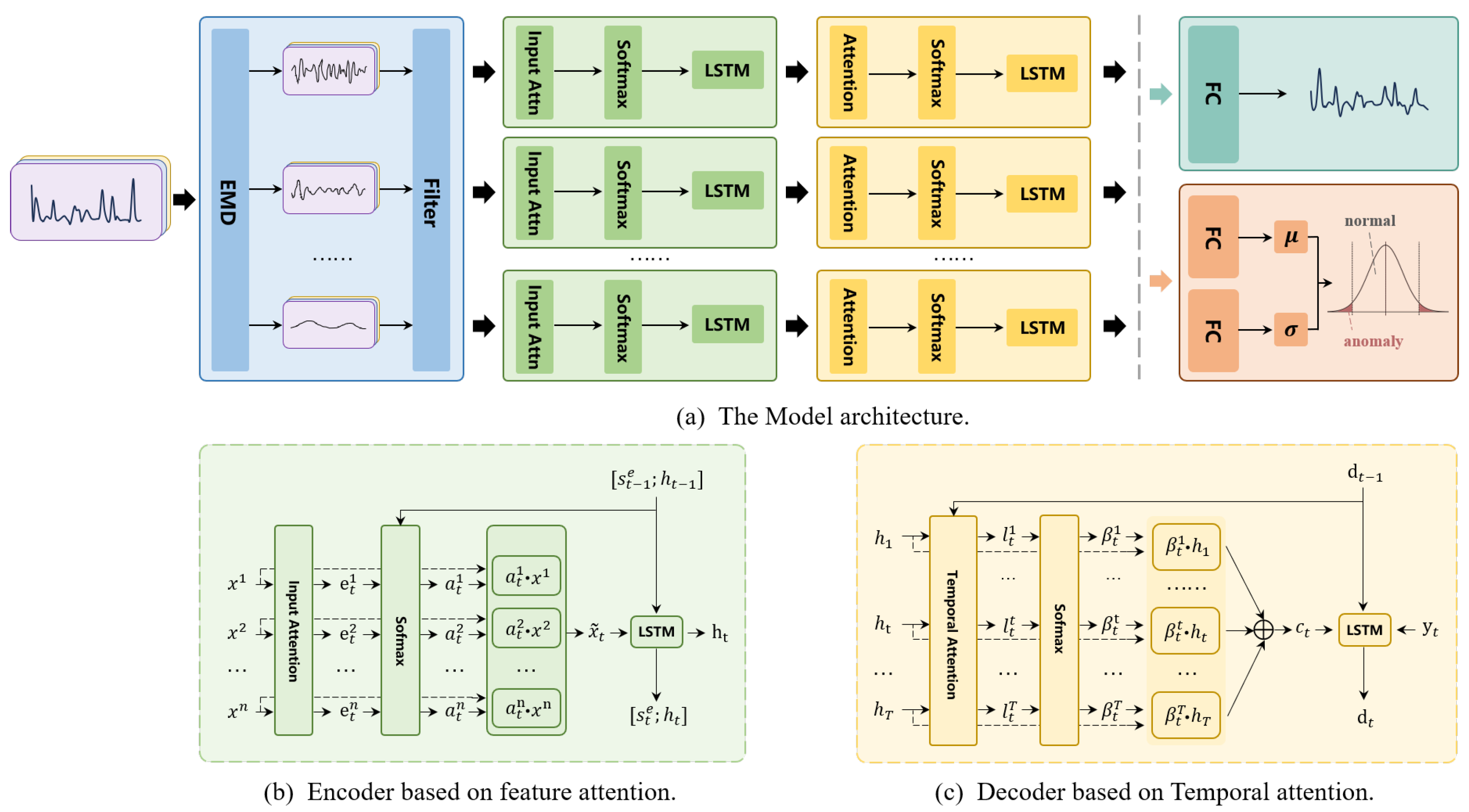
This section provides a detailed description of the model, as illustrated in Figure 1. Traffic signals in industrial networks are typically composed of multiple sources, characterized by high complexity and diversity. These sources differ not only in frequency but also in their variation patterns, fluctuation characteristics, and periodicity. To address this complexity, we first employ the HHT’s EMD algorithm to decompose the original traffic signals into multiple components. These components capture different modes of the traffic signals, including rapid fluctuations, periodic variations, and long-term trends. The components of different frequencies are treated as independent inputs for the subsequent traffic prediction module. The traffic prediction module comprises an encoder based on feature attention mechanisms and a decoder leveraging temporal attention mechanisms. The encoder extracts features from each frequency component and dynamically adjusts weights based on feature importance to generate weighted feature representations. This process enables the model to focus on signal components that are more critical for traffic prediction. For instance, low-frequency stable signals may be more important for trend prediction in certain devices, while high-frequency bursts might be key for anomaly detection in others. Subsequently, the decoder employs an LSTM network to capture both long-term and short-term dependencies in the signals. By incorporating temporal attention mechanisms, the decoder outputs traffic predictions for future time intervals. Finally, we introduce a dynamic threshold anomaly detection module based on a statistical window. This module calculates residuals in real time and adjusts thresholds dynamically based on the distribution of historical residuals. This approach effectively accommodates the variability and diversity of traffic signals in industrial networks, enabling the reliable identification of anomalous fluctuations in traffic data.
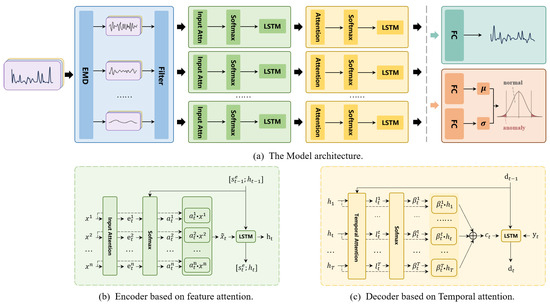
Figure 1.
The architecture and modules.
3.1. Signal Decoupling Module
When dealing with complex data from multiple sources, conducting detailed decomposition and analysis of the data becomes critically important. Breaking data into finer-grained components allows for a clearer identification of their intrinsic features and patterns, while significantly enhancing the robustness and adaptability of the model [33]. In industrial control networks, traffic signals may exhibit periodic fluctuations, sudden changes, and long-term trends, which are typically nonlinear and non-stationary. Additionally, changes in input conditions (e.g., voltage fluctuations) may introduce high-frequency noise or transient interference signals. Therefore, extracting and utilizing information from traffic data across different frequencies is crucial for the accuracy of time-dependent modeling.
To achieve signal separation, this study employed the HHT. The core component of the HHT is EMD, which was introduced by Huang et al. EMD decomposes a signal into a series of Intrinsic Mode Functions (IMFs) based on the signal’s local frequency characteristics [34]. This method excels in analyzing nonlinear and non-stationary signals that are challenging for traditional approaches and is particularly well suited for handling complex, multi-source traffic signals in industrial networks. In using EMD within the HHT framework, the raw traffic signals are decomposed into multiple IMF components, effectively separating sub-signals with distinct characteristics and origins. Each IMF component represents features within a specific frequency range. High-frequency IMF components typically correspond to sudden, short-term fluctuations and are effective at capturing transient noise caused by input condition changes, such as voltage fluctuations. In contrast, low-frequency components reflect the long-term trends or slow variations in the signal. This decomposition approach allows the model to isolate different change patterns within the signal, enabling it to suppress interference from input conditions and focus more on the unique features of each signal component.
The core idea of EMD is to decompose a signal into a series of IMFs, each representing a localized oscillatory mode. Each IMF must satisfy two conditions: (1) the number of extrema and the number of zero-crossings must either be equal or differ by at most one, and (2) the mean of the upper and lower envelopes, defined by the local maxima and minima, must be zero. With the EMD method, industrial control traffic data can be iteratively decomposed into a series of components. The specific steps are as follows.
First, identify the local extrema in the signal and construct the upper envelope and the lower envelope through interpolation. Then, subtract the mean of the envelopes from the original signal to obtain the first component :
If the component exhibits asymmetry or additional extrema, it undergoes iterative smoothing until it satisfies the IMF criteria. This process is repeated iteratively, where each sifting step calculates the mean of the envelopes and subtracts it from the signal. The iterations continue until the remaining signal becomes symmetric and contains no new extrema, i.e., no further IMF components can be extracted. Specifically, the process of extracting components from the original signal is as follows [35]:
Here, denotes the signal after the k-th iteration, while and represent the upper and lower envelopes, respectively, at the k-th iteration. is the first extracted IMF component, and is the residual signal after removing . After k iterations, the original signal can be represented as the sum of multiple IMF components and a residual term .
Next, the time series is reconstructed by designing filters to select a subset of components as the desired signal, while discarding unnecessary parts. This process effectively smooths and filters the signal. Based on the results of the EMD, the extracted modes—IMF1, IMF2, IMF3, IMF4, etc.—represent signal components at different frequency bands. If the number of modes obtained from EMD exceeds five, IMF5 and all subsequent modes are merged and treated as a single composite high-frequency local oscillatory mode. Conversely, if the number of modes is fewer than five, zero sequences are appended to ensure that the final number of modes is fixed at five.
Furthermore, these decomposed feature signals are transformed into higher-dimensional representations , providing richer feature representations for the subsequent spatiotemporal network model. This process enhances the model’s performance by leveraging a more comprehensive set of features.
3.2. Traffic Prediction Models
After decoupling the original traffic signal into traffic sub-signals of different frequencies, these components are fed into the prediction model for forecasting. The prediction model primarily consists of a feature-attention-based encoder and a time-attention-based decoder, designed to adaptively capture and integrate dependency features between long-term and short-term sequences across different frequencies.
3.2.1. Encoder Based on Feature Attention
To enhance the model’s ability to focus on different signal components, we introduce an input attention mechanism. As shown in Figure 1a, the feature-attentive encoder adaptively selects the most relevant feature sequences. In analyzing the characteristics of each input signal, the encoder dynamically adjusts the importance weights of features, enabling the model to focus more effectively on the most informative components for prediction in complex signal scenarios.
For a given original signal , the signal decoupling process produces a new signal matrix (e.g., , collectively denoted as ), where . Here, represents the values of the m-th frequency signal at each time t, and T is the length of the time series. Additionally, denotes the combination of all feature components at time t.
In time series modeling, Long Short-Term Memory (LSTM) networks are widely used for various sequence prediction tasks due to their ability to effectively capture long-range dependencies. Specifically, at each time step, the LSTM processes the current input along with the previous hidden state . Through a forget gate , it decides which information should be discarded, while an input gate determines which new information should be stored, and an output gate generates the current output based on the updated memory cell. These gating mechanisms work together, allowing the LSTM to dynamically adjust the flow of information based on the varying needs at each time step, thus enabling the precise modeling of time series characteristics. Specifically, the operations of an LSTM unit are as follows [36]:
Here, , , , and , , represent the learnable weight parameters and bias terms for the forget, input, and output gates, respectively. and are the learnable weight parameters and bias terms for the memory cell. The notation denotes matrix concatenation. ⊙ denotes element-wise multiplication. represents the Sigmoid activation function. The LSTM gating mechanism uses the Sigmoid function to generate values between 0 and 1, effectively controlling the flow of information. This is crucial for handling the non-stationarity of ICS traffic, as it allows for dynamic, input-dependent, adaptive gating.
Based on the original signal and the signals decomposed into different frequency components, an encoder is constructed using feature attention. By dynamically assigning weights to the signals of different frequencies, the encoder can adaptively optimize the representation of input features. This allows the model to automatically focus on the most relevant frequency components during training, enhancing its ability to model time series data effectively.
Given the m-th frequency signal , the attention score is computed using a two-layer perceptron. This score not only takes into account the feature value at the current time step but also incorporates the historical information from the encoder LSTM network, including the previous hidden state and the cell state .
where , , and are the learnable weight parameters, and is the bias term. The attention score is normalized using the Softmax function:
The obtained attention weight represents the importance of the m-th frequency signal at time step t. Next, a new feature representation is generated by weighting the original signal input :
The weighted feature representation is then fed into the LSTM network, and after processing through the LSTM, the set of hidden states is output. Each hidden state corresponds to the weighted representation of the features at time step t:
3.2.2. Decoder Based on Temporal Attention
In time series modeling, both the time scale of historical data and the selection of features play a critical role in the performance of the model. Therefore, in the decoder, we use an LSTM network to capture long-term dependencies. However, the LSTM relies solely on the flow of information in a time-sequential manner and does not dynamically focus on which historical information at specific time points is more important for predicting the target sequence. To address this limitation, we introduce a temporal attention mechanism, which dynamically assigns weights to key time steps, as illustrated in Figure 1b. This mechanism is driven by a two-layer perceptron and the historical information encoded by the LSTM. At each time step t, the corresponding temporal attention score is calculated:
where , , and are the learnable weight parameters of the two-layer perceptron in the decoder, and are the hidden state and memory cell state of the decoder LSTM at the previous time step, respectively, and is the attention-weighted output. Then, the temporal attention scores are converted into temporal attention weights using the Softmax function, which quantifies the importance of the corresponding information at different time points in the decoder:
Finally, by performing a weighted average of the encoder outputs across all time steps, the result is obtained:
aggregates the key information learned from different time steps and reflects the temporal attention results on the input feature matrix. It is then fed into the decoder LSTM network for iteration. At each time step, the decoder LSTM updates its information by incorporating , generating a new hidden state. The update process of the decoder LSTM can be expressed as [36]
where , , , and , , are the learnable weight parameters and bias terms for the forget gate, input gate, and output gate, respectively. and are the learnable weight parameters and bias terms for the memory cell. The notation represents matrix concatenation, denotes the sigmoid activation function, and ⊙ indicates element-wise multiplication. In the industrial control flow prediction task, we directly use a fully connected layer to fuse the state vectors , obtained by processing different frequency signals, and predict the flow value at the next time step.
3.3. Anomaly Detection Method Based on Deep Probability Prediction
Although constructing an efficient traffic prediction model is the foundation of this study, our ultimate goal is to achieve high-precision real-time anomaly traffic detection for industrial control systems. Due to the complex and dynamic nature of traffic in industrial control systems, traditional static threshold detection methods are often inadequate and fail to maintain high detection accuracy. To address this issue, this study constructed a deep probabilistic detection module to replace the fully connected layer in the prediction model for anomaly traffic detection. The details of this module are as follows:
As shown in the lower right corner of Figure 1a, to estimate the trend and oscillatory patterns of the conventional flow, we use the final output from the decoder LSTM as input. This input passes through two independent fully connected layers, each predicting the possible distribution of the flow value at the current time step. We assume that the flow follows an overall distribution, where the outputs of the two fully connected layers correspond to the mean and standard deviation , respectively.
We can then define the conditional probability distribution at each time step as
To optimize the model parameters, we adopt a loss function based on maximum likelihood estimation, where the objective is to maximize the log-likelihood of the true value X under the predicted distribution . Specifically, for positive samples (i.e., normal traffic without anomalies at the current time step), the objective is to minimize the following negative log-likelihood loss function:
Additionally, to improve the training efficiency of the model, we introduce negative samples (i.e., pre-labeled anomalous traffic) within the same training batch. Let the anomalous data of the negative samples be denoted as . For the negative samples, we can similarly define an anomaly loss function to minimize their likelihood under the model’s predicted distribution:
The final total loss function, combining the loss from normal and anomalous samples, is given by
where is a weight parameter used to balance the contribution of normal and anomalous samples to the total loss. In this way, the model can optimize for normal predictions while enhancing its sensitivity to anomalous data through training on the anomalous samples, achieving high-precision real-time anomaly detection.
4. Experiments and Results
In this section, we evaluate the performance of the proposed algorithm in traffic prediction and anomaly detection tasks through a series of experiments. We first introduce the dataset and evaluation metrics, followed by a comparative analysis with baseline models and ablation studies. We used real-world datasets to compare our method with several baseline models to validate its effectiveness.
4.1. Experimental Setup
4.1.1. Dataset
This study used network traffic data from a production-level industrial control system (Site M) in an oilfield as the experimental dataset. First, by processing passively captured network traffic in PCAP format, we constructed the network traffic dataset for Site M, which includes both TCP and UDP traffic. Using packet header information, we performed protocol recognition and classification on the captured traffic. The identified protocol types included ARP, TCP/IP, DNP3, HTTP, TLS, and UDP. The classified traffic is grouped and stored by protocol type for subsequent processing. Subsequently, we selected ten standard traffic features listed in Table 1, covering key metrics such as average packet length, packet count, and average segment size. For each protocol type, these feature values are computed; for example, the average packet length is obtained by calculating the mean of all packet lengths, and packet count is determined by counting the number of packets within a specific time window. Additionally, we applied the EMD method from HHT to decompose the raw traffic signals into multiple IMF components. This process separates the sub-signals of different components and features, isolating various changing patterns in the signal, thus providing richer feature representations for the subsequent network model.

Table 1.
The list of traffic characteristics.
The experimental dataset includes traffic data from Remote Terminal Units (RTUs), programmable logic controllers (PLCs), and Supervisory Control and Data Acquisition (SCADA) systems, as these components play a core role in oil and gas industrial control networks. RTUs are primarily used for data acquisition and remote control at well sites and metering stations, PLCs are used for equipment and process control at large station sites, and SCADA serves as the central monitoring system for the entire production process. These devices are highly interconnected in industrial control networks, with critical responsibilities, making them essential objects to consider in network security analysis.
To visually present the variation in network traffic features over time at Site M, Figure 2 shows the trend in three key traffic features of packets sent and received by industrial control devices over 10,000 time steps (each time step being 10 s, with a total duration of 100,000 s). Additionally, the figure illustrates the results of decomposing one of the features using the EMD method, revealing the fine-grained dynamic changes in the feature in the time dimension.
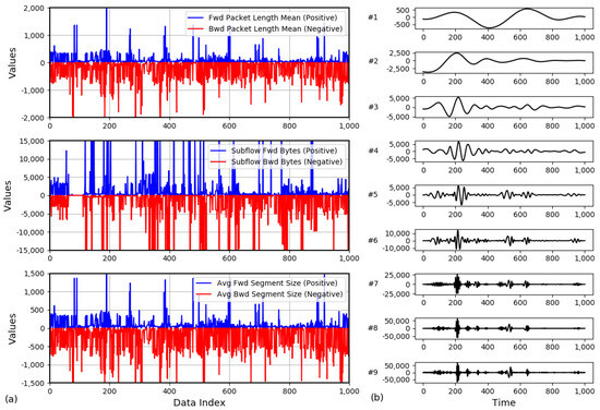
Figure 2.
(a) A snapshot of the time series measurement of the traffic characteristics. (b) Example of Empirical Mode Decomposition(EMD) decomposition.
Figure 2a presents three snapshots of different traffic feature measurements, reflecting the dynamic changes in various industrial control network traffic features along the time dimension. These snapshots reveal the diversity of network traffic, including volatility, burst events, and periodic fluctuations, providing crucial data support for traffic prediction.
Figure 2b illustrates the process of EMD applied to the feature signal, demonstrating how the EMD method decomposes complex traffic feature signals into multiple IMFs and a trend component. This method decomposes the signal features into multiple frequency bands, enabling a more in-depth analysis of the dynamic variations in each frequency band. This process aids in a more accurate understanding of the components within the traffic signal, thus enhancing the accuracy of network traffic prediction models.
4.1.2. Parameter Setting and Evaluation Indicators
The experimental environment was based on Python 3.6, using Pytorch 1.10.2 as the deep learning framework, and was run on a server equipped with an Nvidia GeForce RTX 4090 GPU (Nvidia Corporation, Santa Clara, CA, USA).
The model training utilized the Adam optimizer, with a learning rate set to 0.001, a maximum of 500 training epochs, and a batch size of 64. During training, the mean absolute error (MAE) was used as the loss function. To prevent overfitting, an early stopping mechanism was employed, where training was terminated early if the validation loss did not decrease for 20 consecutive epochs. All experiments were repeated five times, and the average of the evaluation metrics was used as the final result.
To evaluate the performance of the prediction model, two common traffic prediction metrics were used: MAE and Mean Absolute Percentage Error (MAPE). Their specific definitions are as follows:
In the above formulas, represents the i-th actual value, represents the i-th predicted value, and represents the set of observed samples. MAE evaluates the prediction accuracy by calculating the average of the absolute differences between the predicted and actual values. MAPE calculates the relative percentage of prediction errors, which helps reduce the impact of unit differences.
Furthermore, to evaluate the performance of the intrusion detection algorithm used, the commonly employed evaluation metrics in intrusion detection of precision and recall were used. In addition, to provide a more comprehensive, objective, and accurate assessment of the model’s effectiveness, we introduced the F1 score. Their specific definitions are as follows:
In these formulas, represents the number of true positive samples correctly predicted as positive by the model. represents the number of true negative samples correctly predicted as negative by the model. represents the number of false positive samples where the model incorrectly predicts negative samples as positive. represents the number of false negative samples where the model incorrectly predicts positive samples as negative.
4.1.3. Baseline
We compared the predictive model proposed in this paper with a series of baseline models for time series forecasting, including traditional methods and classic deep learning approaches. All these baseline models have publicly available official code. The baseline models were as follows:
HA: A classic time series modeling method focused on handling data with trend and seasonality patterns, capable of effectively capturing the variation patterns in time series data [37].
VAR: A classical statistical model widely used in time series forecasting tasks. By establishing the linear dynamic relationships between multiple variables, the VAR model captures the autocorrelation and interaction within time series data, making it suitable for analyzing the interdependencies of variables and forecasting the future trends of multivariate systems [38].
SVR: A support vector machine (SVM)-based method that performs regression by mapping the data into a high-dimensional space and finding the optimal regression hyperplane in that space [39].
RNN: A deep learning model for sequential data that captures the temporal dependencies by sharing parameters across time steps, making it suitable for time series forecasting and other similar tasks.
LSTM: An improved version of the RNN that introduces memory cells and gating mechanisms, effectively capturing long-range dependencies and overcoming the vanishing gradient problem in long-sequence modeling [36].
TCN: A time series modeling method based on convolutional neural networks (CNNs) that captures long-term dependencies through causal convolutions and dilated convolutions. It offers good parallelism and more flexible receptive field adjustments [40].
Transformer: A neural network model based on a self-attention mechanism and positional encoding that effectively captures long-range dependencies and is widely used in time series forecasting tasks [41].
The baseline models selected include both traditional statistical methods and modern deep learning models to reflect the comparative effectiveness of various modeling paradigms. Specifically, HA and VAR are classic time series models based on data stationarity and linear dependency assumptions, illustrating the boundaries of traditional methods in complex industrial control scenarios. SVR, as a kernel-based regression model, can handle nonlinear relationships but lacks the capability to model temporal dependencies. RNN and LSTM, as recurrent neural networks, are adept at handling short-term temporal dependencies but have limitations in capturing long-distance, multi-scale dynamics. TCN uses dilated convolutions to model long-term dependencies and is relatively lightweight in structure. The Transformer introduces self-attention mechanisms to dynamically weight features at different time steps, exhibiting superior performance in time series prediction tasks.
4.2. Experimental Results and Analysis of Predictive Models
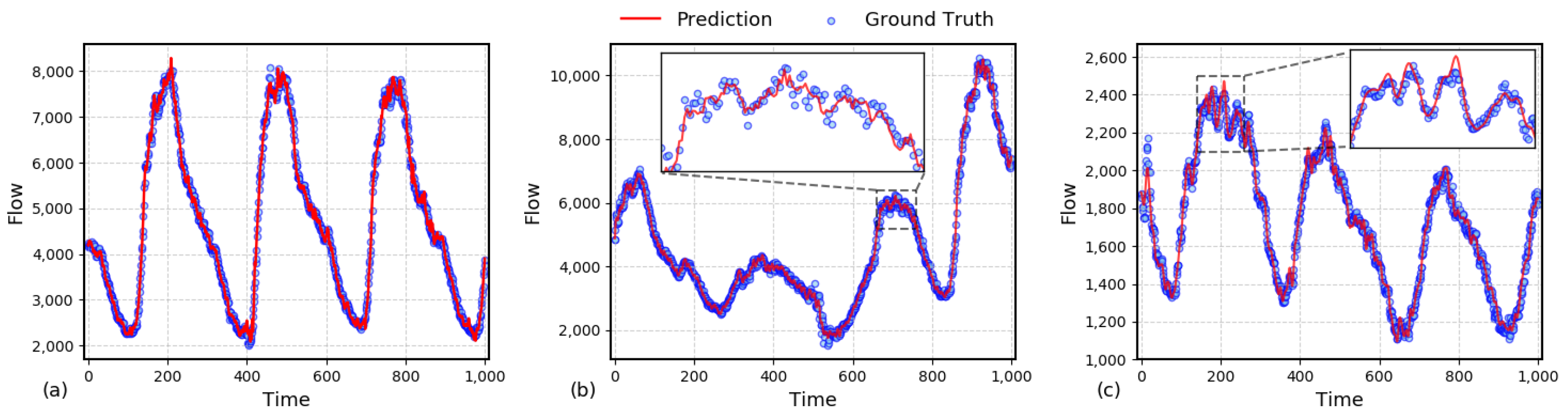
To provide a more intuitive demonstration of the proposed algorithm’s performance in traffic prediction, we randomly selected three sets of continuous prediction results from the test dataset. Each set adopts a sliding window approach to dynamically predict traffic at the next time step. The red solid line represents the predicted results, while the blue dots indicate the actual traffic data. From Panel (a) in Figure 3, it can be observed that the proposed algorithm achieves high prediction accuracy for low-frequency signals, reflecting trends over larger time scales. Panels (b) and (c) zoom in on the local prediction details of high-frequency oscillatory traffic signals. The inset figures reveal that, because the proposed method processes traffic signals of different frequencies separately, the algorithm is able to fit oscillatory signals over smaller time scales to a certain extent. To prevent the model from becoming overly complex due to fine-grained divisions and considerations of signals across various frequencies, we discarded a portion of high-frequency signals, some of which may include white noise. This trade-off is a key reason why the algorithm cannot perfectly fit all actual data points. Overall, the selected cases demonstrate that the proposed traffic prediction model excels in capturing both global trends and local fluctuations. This advantage is primarily attributed to the series of operations involving signal decomposition, separate processing, and coupled prediction.
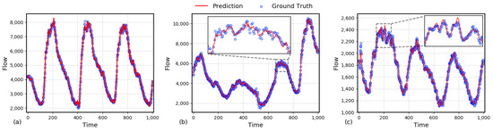
Figure 3.
(a) Comparison of predicted and true values for traffic. (b) Zoom-in view I of local prediction for high-frequency traffic oscillations. (c) Zoom-in view II of local prediction for high-frequency traffic oscillations.
After a visual analysis of the prediction results, Figure 4 presents the overall performance of the algorithm from a statistical perspective. Each point in Figure 4a represents a predicted sample from the test set. Clearly, the closer the distribution of the data is to the diagonal line , the higher the prediction accuracy. First, we use Pearson and Spearman correlation coefficients to quantify the distribution differences between the predicted and actual data. From Panel (a), it can be observed that the Pearson correlation coefficient (p-value < 0.05) and the Spearman correlation coefficient (p-value < 0.05), indicating a high linear correlation between the model’s predicted flow values and the actual flow values. This suggests that the model has a strong capability in capturing the flow trend.
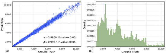
Figure 4.
(a) Scatter plot of true and predicted values. (b) Histogram of the distribution of true values.
Furthermore, it is worth noting that as the absolute values of the flow data increase, the distribution of the predicted data gradually deviates from the diagonal, indicating that the variance of the predicted values increases. This is mainly because the distribution of the training and testing samples is not uniform across the range of predicted values. As shown in Panel (b), the probability density of the sample size decreases significantly as the absolute value of the predicted flow increases, meaning the prediction model faces an imbalanced sample distribution during both the training and testing phases. Since there are fewer training samples in the high-value regions, the model’s generalization ability in these areas is relatively weaker, which may result in higher prediction errors.
To evaluate the advantages of the proposed algorithm in traffic signal analysis and prediction, we compared it with several classical deep learning models widely used in time series prediction tasks. The results are shown in Table 2. The proposed method significantly outperforms the baseline models in terms of both the MAE and MAPE metrics. Firstly, as observed in the table, traditional time series analysis methods such as HA and VAR rely on assumptions of stationarity and linearity. Since industrial control network traffic data typically exhibit nonlinear and complex time-varying characteristics, these methods fail to effectively capture critical changes in the data. SVR (with a Gaussian kernel) demonstrates slight accuracy improvements after adequate training, but its error rate remains higher than RNN’s because SVR concatenates all input features without leveraging temporal factors. Notably, RNN predictions exhibit slightly greater fluctuations compared to those of SVR. With the ability to consider temporal factors and multiple features simultaneously, TCN and LSTM achieve better accuracy. In particular, LSTM, with its effective gating mechanism, achieves the best accuracy among these methods, which is the primary reason why the proposed algorithm employs LSTM for handling temporal features. In recent years, the Transformer architecture, based on attention mechanisms, has proven to be the most efficient feature fusion algorithm in fields such as image recognition, natural language processing, and large-scale models. To enhance its temporal feature utilization, we introduced a positional encoding into the input features at each time step. The results validate that the attention mechanism is effective for traffic prediction tasks, as it captures the complex relationships between traffic at the next time step and features from different historical moments. This serves as the theoretical basis for using attention mechanisms in the proposed algorithm. By integrating the attention mechanism with a time series decomposition module, the proposed algorithm achieves superior performance in both prediction accuracy and stability compared to the baseline models. This is made possible by the dual-stage attention coupling architecture in our proposed algorithm. The signal decoupling module decomposes the raw traffic signals into multiple frequency components, significantly improving the precision of temporal feature extraction. The feature attention module dynamically adjusts the importance weights of each feature, enabling the model to focus precisely on the most influential features for prediction. This not only reduces the complexity of feature fusion but also enhances the prediction accuracy of individual frequency channels. Furthermore, the temporal attention module captures both long- and short-term dependencies in the traffic signals, further enhancing the model’s ability to handle complex temporal data. The synergistic effect of this architecture results in exceptional performance in traffic signal analysis and prediction.
Table 2.
Comparison of the prediction method with the baseline model (mean ± 2 times the standard error of the mean).
To further evaluate the performance of the proposed model in traffic prediction, we analyzed the impact of three hyperparameters on prediction accuracy: the length of historical input data, the number of neurons in the hidden layers of the LSTM module, and the prediction horizon. The results are shown in Figure 5, where normalized metrics are used to account for the significant differences in the absolute values of different evaluation measures. Each result is divided by the maximum mean value for better comparability. Firstly, as illustrated in Figure 5a, MAE is more sensitive to the input data length than MAPE. MAE demonstrates a preference for larger input time steps, whereas MAPE exhibits an opposite trend, showing increased errors when the input step exceeds 260. Since MAPE is more sensitive to fluctuations in the data, this result suggests that excessive input data might degrade the model’s generalization performance. On the other hand, too few input steps reduce the model’s accuracy due to insufficient information. Balancing predictive accuracy and computational efficiency, we selected an input sequence length of 200 as the optimal configuration for the model. Secondly, as shown in Figure 5b, we investigated the influence of the number of LSTM hidden neurons, ranging from 128 to 1024, on prediction accuracy. Overall, as the number of hidden neurons increases, all metrics exhibit a trend of initial stability followed by a sharp rise. This indicates that beyond a certain number of neurons, the model may overfit the training data, leading to a decline in predictive performance. Additionally, adding too many hidden neurons not only fails to significantly improve accuracy but also increases computational overhead. Consequently, we configured the LSTM module with 128 hidden neurons for testing and evaluation. Finally, we examined the effect of prediction horizon on model performance. Figure 5c displays the variation in MAE and MAPE as the prediction length increases from 1 to 10. The results show that as the prediction horizon grows, the model’s accuracy decreases, and prediction instability increases significantly. This is due to the strong nonlinear characteristics and complex time-varying patterns of traffic data, which make long-term predictions exponentially more challenging. Considering our ultimate goal of real-time detection of anomalous traffic at the next time step, we selected a prediction horizon of 1 as the model’s configuration.
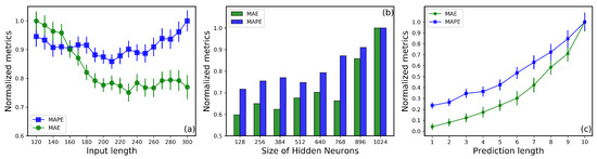
Figure 5.
(a) Impact of input sequence length on prediction performance metrics. (b) Variation of evaluation metrics with the number of Long Short-Term Memory(LSTM) hidden units. (c) Variation of evaluation metrics with prediction horizon length.
4.3. Experimental Results and Analysis of Anomaly Detection Methods
In the previous section, we discussed in detail the performance of our proposed new algorithm for the task of predicting future traffic, where the prediction model uses a single fully connected layer to map the hidden state to future traffic dynamics. To meet the requirements of anomaly detection for industrial control traffic data, we innovatively proposed a deep probabilistic prediction-based anomaly detection method. To comprehensively utilize the normal traffic data used in the prediction task and improve the model’s training effectiveness, we employed a transfer learning strategy by dividing the training of the anomaly detection model into three phases. In the first phase, we train a prediction model following the same procedure as the prediction model. In the second phase, to leverage the feature extraction and processing capabilities of the backbone model for industrial control traffic data, we replace only the fully connected layer with a new deep probabilistic estimation layer, fixing the parameters of the backbone network, and train on the anomaly dataset. In the third phase, we fine-tune the model with minimal training effort on the training set. The performance analysis of the anomaly detection model is shown in Figure 6.
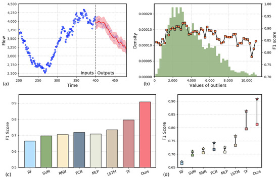
Figure 6.
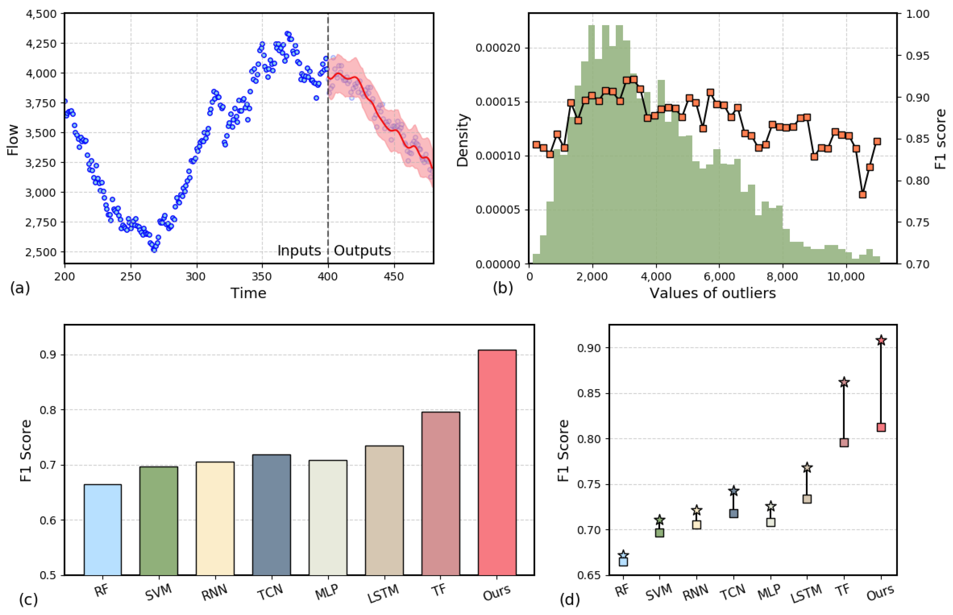
(a) Probability distribution prediction result plot. (b) Histogram of outlier distribution and its F1 score. (c) Graph of the F1 score of the anomaly detection model. (d) Abnormal detection performance comparison chart. (Square points represent models combined with the static threshold method, while star points indicate models combined with the probability forecasting method).
Figure 6a presents the probabilistic distribution prediction results of the method we proposed. On the left are the input data, and on the right is the predicted output, where the shaded region represents twice the variance estimated by the deep probabilistic prediction module. It is important to note that when detecting anomalies, we focus more on the factual detection accuracy, i.e., the probability distribution of traffic at the next time step. Therefore, the predicted results in Figure 6a were computed by sliding the input window over the real historical data, rather than from a single input. For example, in the randomly selected case shown in Figure 6a, we observe that the actual values of the industrial control traffic generally fall within the predicted interval. This indicates that the model can provide a reliable prediction range for most time steps, covering the local uncertainty in the normal traffic data. This confirms the advantages of our proposed anomaly detection model, which, when handling complex industrial control traffic signals, is able to effectively fit both the overall trend of the time series data and high-frequency oscillations. Compared to point estimation, probabilistic estimation offers superior learning and fitting capabilities for anomaly detection tasks, which is one of the key reasons for the performance advantage of our method.
As the anomaly data we collected also suffer from data imbalance, similar to the issue shown in Figure 4, Figure 6b illustrates the performance of our algorithm when faced with different magnitudes of anomaly values. The bar chart represents the distribution of the number of anomalies, while the line chart depicts the F1 scores corresponding to different anomaly value ranges. The results show that when the anomaly values are smaller, the F1 score for detection is higher. On one hand, this is due to the higher occurrence probability of anomalies in this range, ensuring ample training samples. On the other hand, it also demonstrates that our anomaly detection model is capable of identifying anomalies at smaller traffic scales. However, when the anomaly values are larger, the F1 score slightly decreases. This phenomenon can be attributed to insufficient data, where the model struggles to fully capture the regularities and uncertainties of the data.
Figure 6c compares the anomaly detection performance of several baseline models in the industrial control network scenario. It should be noted that these baseline models all use traditional static threshold detection methods, where the trained prediction model is combined with a tunable anomaly detection threshold. If the difference between the predicted value and the observed value exceeds this threshold, the traffic signal is considered anomalous. Compared to traditional methods (such as RF [42], SVM [43], MLP, etc.) and deep learning models based on time series features (such as RNN, TCN, LSTM, and Transformer), our proposed probabilistic distribution prediction method achieves the highest F1 score of approximately 0.91. Among them, the RF, SVM, and MLP methods perform relatively poorly, mainly because these methods cannot effectively capture the dynamic characteristics of time series data in the complex industrial control network scenario. SVM and RNN show slight improvement but are still limited by the model’s feature extraction capabilities. The LSTM and Transformer models perform well in capturing temporal relationships, leading to relatively high F1 scores. However, their identification accuracy still slightly lags behind that of our method, mainly because they lack the ability to decouple complex temporal features and model the interrelationships between features. Specifically, the LSTM and Transformer models fail to sufficiently decouple temporal features of different frequencies, making it difficult to capture the joint characteristics of low-frequency trends and high-frequency spikes when processing complex industrial control network traffic. Additionally, these models are limited in modeling feature interrelationships, failing to fully exploit the complex relationships between features, which impacts anomaly detection accuracy. In contrast, our method effectively addresses these issues by incorporating a time series decomposition module and feature attention mechanism, resulting in enhanced anomaly detection performance.
Further analysis reveals that the false positive rate is mainly caused by two situations. First, traffic pulse signals generated by industrial equipment during normal high-frequency operations (such as rapid state switching or fast polling requests in the DNP3 protocol). Due to the similarity of high-frequency characteristics with attack behaviors, although the EMD decomposition can extract high-frequency components (IMF1-IMF3), the model’s coverage of normal high-frequency patterns is insufficient, leading to misclassification. The second cause is low-frequency environmental noise (such as sporadic sensor interference), which after EMD decomposition remains as low-frequency IMF components (such as IMF4-IMF5), with their gradual variation being misidentified by the model as potential anomalies. The false negative rate is primarily concentrated in high-amplitude anomalous traffic and covert protocol attacks (such as BlackEnergy masquerading as DNP3 protocol interactions). High-amplitude anomalous traffic is underrepresented in the training data distribution, leading to inadequate modeling of its probability distribution and increasing the risk of false negatives. Covert protocol attacks exploit protocol semantic imitation (e.g., matching the sequence features of normal operations), thereby reducing residual abnormality and making it difficult for the model to distinguish between normal behavior and attacks, which further exacerbates the false negative rate.
To further investigate the impact of the deep probabilistic detection module on anomaly detection accuracy, we present a set of simple ablation experiments in Figure 6d. The experiments compare the performance differences in anomaly detection when using the deep probabilistic distribution prediction (PF) head and the static threshold detection (ST) method with different backbone models. In the figure, square markers represent the results of models combined with the ST method, while star markers represent the results of models combined with the PF method. The results show that algorithms such as RF, SVM, MLP, and RNN, due to poor basic prediction performance, show only a slight increase in F1 score when using the PF detection method, but the overall detection accuracy remains low. On the other hand, the TCN, LSTM, and, especially, Transformer models show significant improvements in anomaly detection accuracy after combining with the PF method. This indicates that our deep probabilistic prediction module is effective for anomaly detection tasks. Finally, it is worth noting that while our method (ours) achieves approximately 0.91 detection accuracy, if the detection method is replaced with ST, the detection accuracy is only about 0.018 higher than that of the Transformer. This result confirms that, although the accuracy of the backbone prediction model is fundamental for real-time anomaly detection, the deep probabilistic estimation-based detection method is more effective at capturing uncertainty information in the traffic data. It provides an adaptive dynamic detection standard for anomaly detection tasks, significantly improving detection accuracy. In summary, our proposed anomaly detection algorithm is crucial for addressing issues such as the dynamic evolution of equipment combinations and environmental changes that may occur in industrial control networks.
Although a quantitative comparison with ICS-specific custom models was not feasible due to the lack of publicly available implementations, we conducted a qualitative assessment to highlight the strengths of our proposed method. For example, MERLIN [19] focuses on subsequence anomaly detection but lacks the ability to perform multi-scale frequency analysis. SOM-DAGMM [29], on the other hand, struggles to capture long-term temporal dependencies. In contrast, our method leverages HHT-based signal decomposition and cross-frequency attention mechanisms to explicitly model both low-frequency trends and high-frequency bursts, enabling finer-grained anomaly detection. Moreover, unlike the static thresholding approach proposed in [22], our deep probabilistic estimation module dynamically adapts to traffic fluctuations, offering greater adaptability in real-world ICS environments.
5. Discussion
The multi-feature time series dataset used in this study assumes that all traffic features are fully visible and that there are no missing data issues. However, in real-world industrial control systems (ICSs), data are often incomplete or features may be invisible due to factors such as traffic encryption, privacy protection, or sensor anomalies. Under such imperfect data conditions, the performance and robustness of the deep learning detection model proposed in this paper require further investigation and validation.
Regarding scalability, the model can process 1800 traffic records per second (each record contains 10 features as listed in Table 1) on an Nvidia GeForce RTX 4090 GPU, with an inference delay of less than 5 milliseconds. Since industrial control networks typically feature low bandwidth and high real-time requirements (e.g., the Modbus TCP typical communication frequency is 10–100 Hz), the current processing speed is sufficient to meet the demands of most scenarios. Additionally, the model supports parallel processing, and throughput can be further improved by adjusting the batch size.
Although the deep learning model proposed in this study achieves high accuracy in anomaly detection for industrial control networks, there are still limitations that require further exploration. In edge device deployment scenarios, architectures relying on high-performance GPUs may face energy efficiency bottlenecks. It is noteworthy that while environmental factors such as temperature may indirectly affect network behavior through hardware performance, the dataset used in this study focuses on network traffic metadata and protocol features and does not include physical sensor measurements such as temperature and humidity. This limits the model’s ability to recognize anomalies triggered by physical environmental changes. Future work will combine power consumption optimization with functionality enhancement strategies, such as dynamic channel pruning to compress computational redundancies and designing dedicated pipelines to accelerate the HHT and LSTM modules. This will reduce energy consumption while supporting batch processing. Additionally, functionality can be enhanced by incorporating physical sensor data alongside network traffic features to build a more comprehensive anomaly detection framework, systematically improving detection robustness in complex industrial scenarios.
The multi-scale feature fusion anomaly detection method proposed in this paper demonstrates significant advantages in performance compared to existing commercial solutions. Commercial systems typically rely on static rule engines or shallow machine learning models, which depend on predefined attack signatures and fixed thresholds, making them less adaptable to the non-stationary and dynamically evolving characteristics of ICS traffic. However, commercial solutions are more mature in terms of protocol compatibility (e.g., supporting OPC UA) and interactive visualization design. The model proposed in this paper is currently tailored to specific oilfield equipment (RTU/PLC/SCADA) and will need to expand its protocol library and optimize its deployment for engineering use in the future.
6. Conclusions
Industrial control systems (ICS) play a crucial role in critical infrastructure, but their security is increasingly threatened by cyberattacks. Existing research on anomaly detection methods in ICSs faces several issues, including poor adaptability to complex traffic patterns, insufficient modeling of time dependencies, and lack of dynamic adaptability in fixed threshold settings. To address these challenges, this paper proposes a real-time monitoring algorithm based on deep learning. The proposed method integrates HHT for signal decoupling, which decomposes traffic signals and extracts time series features at different frequencies. It employs an encoder–decoder structure with feature and temporal attention mechanisms to adaptively capture and fuse long-term and short-term dependency features. Furthermore, the deep probabilistic estimation model is utilized for anomaly detection, enabling real-time adaptation to the variability and diversity of ICS network traffic signals. Experimental results demonstrate that, compared to various traditional and time series-based models, our method achieves the best anomaly detection performance in ICS network scenarios.
Author Contributions
Conceptualization, L.X., K.S., X.Z. and C.Z.; Methodology, L.X. and L.P.; Validation, L.X., K.S. and L.P.; Formal analysis, K.S., X.Z. and C.Z.; Investigation, L.X.; Resources, K.S.; Data curation, X.Z. and C.Z.; Writing—original draft, L.X.; Writing—review & editing, L.P.; Visualization, X.Z.; Supervision, L.P.; Project administration, C.Z. and L.P.; Funding acquisition, L.P. All authors have read and agreed to the published version of the manuscript.
Funding
This work is supported by the National Key Research and Development Plan of China (2023YFC3306100) and SINOPEC Shengli Oilfield Technology Project (YKJ2407).
Data Availability Statement
The data presented in this study are available on request from the corresponding author.
Conflicts of Interest
Author Lin Xu was employed by the company Sinopec. The remaining authors declare that the research was conducted in the absence of any commercial or financial relationships that could be construed as a potential conflict of interest.
References
- Stouffer, K.; Falco, J.; Scarfone, K. Guide to industrial control systems (ICS) security. NIST Spec. Publ. 2011, 800, 16. [Google Scholar]
- Knapp, E.D. Industrial Network Security: Securing Critical Infrastructure Networks for Smart Grid, SCADA, and Other Industrial Control Systems; Elsevier: Amsterdam, The Netherlands, 2024. [Google Scholar]
- Riegler, M.; Sametinger, J. Multi-mode systems for resilient security in industry 4.0. Procedia Comput. Sci. 2021, 180, 301–307. [Google Scholar] [CrossRef]
- Koay, A.M.; Ko, R.K.L.; Hettema, H.; Radke, K. Machine learning in industrial control system (ICS) security: Current landscape, opportunities and challenges. J. Intell. Inf. Syst. 2023, 60, 377–405. [Google Scholar] [CrossRef]
- Lee, M. A Survey on the Real-world Cyberattacks on the Industrial Internet of Things. 2023; Authorea Preprints. [Google Scholar]
- Stoddart, K. Cyberwar: Attacking Critical Infrastructure. In Cyberwarfare: Threats to Critical Infrastructure; Springer: Berlin/Heidelberg, Germany, 2022; pp. 147–225. [Google Scholar]
- Makrakis, G.M.; Kolias, C.; Kambourakis, G.; Rieger, C.; Benjamin, J. Industrial and critical infrastructure security: Technical analysis of real-life security incidents. IEEE Access 2021, 9, 165295–165325. [Google Scholar] [CrossRef]
- Bhamare, D.; Zolanvari, M.; Erbad, A.; Jain, R.; Khan, K.; Meskin, N. Cybersecurity for industrial control systems: A survey. Comput. Secur. 2020, 89, 101677. [Google Scholar] [CrossRef]
- Alladi, T.; Chamola, V.; Zeadally, S. Industrial control systems: Cyberattack trends and countermeasures. Comput. Commun. 2020, 155, 1–8. [Google Scholar] [CrossRef]
- Radicioni, L.; Bono, F.M.; Cinquemani, S. On the use of vibrations and temperatures for the monitoring of plastic chain conveyor systems. Mech. Syst. Signal Process. 2025, 223, 111935. [Google Scholar] [CrossRef]
- Zhang, X.; Zhang, C.; Li, X.; Du, Z.; Mao, B.; Li, Y.; Zheng, Y.; Li, Y.; Pan, L.; Liu, Y.; et al. A survey of protocol fuzzing. ACM Comput. Surv. 2024, 57, 35. [Google Scholar] [CrossRef]
- Fisch, A.T.; Bardwell, L.; Eckley, I.A. Real time anomaly detection and categorisation. Stat. Comput. 2022, 32, 55. [Google Scholar] [CrossRef]
- Abbasi, M.; Shahraki, A.; Taherkordi, A. Deep learning for network traffic monitoring and analysis (NTMA): A survey. Comput. Commun. 2021, 170, 19–41. [Google Scholar] [CrossRef]
- Jiang, J.R.; Chen, Y.T. Industrial control system anomaly detection and classification based on network traffic. IEEE Access 2022, 10, 41874–41888. [Google Scholar] [CrossRef]
- Yuan, X.; Xu, N.; Ye, L.; Wang, K.; Shen, F.; Wang, Y.; Yang, C.; Gui, W. Attention-based interval aided networks for data modeling of heterogeneous sampling sequences with missing values in process industry. IEEE Trans. Ind. Inform. 2023, 20, 5253–5262. [Google Scholar] [CrossRef]
- Shen, W.; Dai, T.; Chen, Z.; Meng, J. CluSAD: Self-Supervised Learning-Based Anomaly Detection for Industrial Control Systems. In Proceedings of the 2024 5th International Conference on Electronic Communication and Artificial Intelligence (ICECAI), Shenzhen, China, 31 May–2 June 2024; pp. 545–552. [Google Scholar]
- Pota, M.; De Pietro, G.; Esposito, M. Real-time anomaly detection on time series of industrial furnaces: A comparison of autoencoder architectures. Eng. Appl. Artif. Intell. 2023, 124, 106597. [Google Scholar] [CrossRef]
- Abdelaty, M.; Doriguzzi-Corin, R.; Siracusa, D. DAICS: A deep learning solution for anomaly detection in industrial control systems. IEEE Trans. Emerg. Top. Comput. 2021, 10, 1117–1129. [Google Scholar] [CrossRef]
- Nakamura, T.; Imamura, M.; Mercer, R.; Keogh, E. Merlin: Parameter-free discovery of arbitrary length anomalies in massive time series archives. In Proceedings of the 2020 IEEE International Conference on Data Mining (ICDM), Sorrento, Italy, 17–20 November 2020; pp. 1190–1195. [Google Scholar]
- Waskita, A.A.; Suhartanto, H.; Persadha, P.; Handoko, L.T. A simple statistical analysis approach for intrusion detection system. In Proceedings of the 2013 IEEE Conference on Systems, Process & Control (ICSPC), Kuala Lumpur, Malaysia, 13–15 December 2013; pp. 193–197. [Google Scholar]
- Moustafa, N.; Creech, G.; Slay, J. Big data analytics for intrusion detection system: Statistical decision-making using finite dirichlet mixture models. In Data Analytics and Decision Support for Cybersecurity: Trends, Methodologies and Applications; Springer: Berlin/Heidelberg, Germany, 2017; pp. 127–156. [Google Scholar]
- Andrysiak, T.; Saganowski, Ł.; Maszewski, M.; Marchewka, A. Detection of network attacks using hybrid. In Proceedings of the Dependability Problems and Complex Systems: Proceedings of the Twelfth International Conference on Dependability and Complex Systems DepCoS-RELCOMEX, Brunów, Poland, 2–6 July 2017; p. 1.
- Yulianto, A.; Sukarno, P.; Suwastika, N.A. Improving adaboost-based intrusion detection system (IDS) performance on CIC IDS 2017 dataset. In Journal of Physics: Conference Series, Proceedings of the 2nd International Conference on Data and Information Science, Bandung, Indonesia, 15–16 November 2018; IOP Publishing: Bristol, UK, 2019; Volume 1192, p. 012018. [Google Scholar]
- Farooq, M. Supervised learning techniques for intrusion detection system based on multi-layer classification approach. Int. J. Adv. Comput. Sci. Appl. 2022, 13, 311–315. [Google Scholar] [CrossRef]
- Song, C.; Sun, Y.; Han, G.; Rodrigues, J.J. Intrusion detection based on hybrid classifiers for smart grid. Comput. Electr. Eng. 2021, 93, 107212. [Google Scholar] [CrossRef]
- Hassan, M.M.; Gumaei, A.; Huda, S.; Almogren, A. Increasing the trustworthiness in the industrial IoT networks through a reliable cyberattack detection model. IEEE Trans. Ind. Inform. 2020, 16, 6154–6162. [Google Scholar] [CrossRef]
- Nassif, A.B.; Talib, M.A.; Nasir, Q.; Dakalbab, F.M. Machine learning for anomaly detection: A systematic review. IEEE Access 2021, 9, 78658–78700. [Google Scholar] [CrossRef]
- Zeng, H.; Zhao, X.; Wang, L. Multivariate time series anomaly detection on improved htm model. In Proceedings of the 2021 IEEE International Conference on Computer Science, Electronic Information Engineering and Intelligent Control Technology (CEI), Fuzhou, China, 24–26 September 2021; pp. 759–763. [Google Scholar]
- Chen, Y.; Ashizawa, N.; Yeo, C.K.; Yanai, N.; Yean, S. Multi-scale self-organizing map assisted deep autoencoding Gaussian mixture model for unsupervised intrusion detection. Knowl.-Based Syst. 2021, 224, 107086. [Google Scholar] [CrossRef]
- Niu, Z.; Yu, K.; Wu, X. LSTM-based VAE-GAN for time-series anomaly detection. Sensors 2020, 20, 3738. [Google Scholar] [CrossRef] [PubMed]
- Boppana, T.K.; Bagade, P. GAN-AE: An unsupervised intrusion detection system for MQTT networks. Eng. Appl. Artif. Intell. 2023, 119, 105805. [Google Scholar] [CrossRef]
- Zhao, H.; Wang, Y.; Duan, J.; Huang, C.; Cao, D.; Tong, Y.; Xu, B.; Bai, J.; Tong, J.; Zhang, Q. Multivariate time-series anomaly detection via graph attention network. In Proceedings of the 2020 IEEE International Conference on Data Mining (ICDM), Sorrento, Italy, 17–20 November 2020; pp. 841–850. [Google Scholar]
- Guo, W.; Wang, J.; Wang, S. Deep multimodal representation learning: A survey. IEEE Access 2019, 7, 63373–63394. [Google Scholar] [CrossRef]
- Van Jaarsveldt, C.; Peters, G.W.; Ames, M.; Chantler, M. Tutorial on empirical mode decomposition: Basis decomposition and frequency adaptive graduation in non-stationary time series. IEEE Access 2023, 11, 94442–94478. [Google Scholar] [CrossRef]
- Hamad, K.; Shourijeh, M.T.; Lee, E.; Faghri, A. Near-term travel speed prediction utilizing Hilbert–Huang transform. Comput. Aided Civ. Infrastruct. Eng. 2009, 24, 551–576. [Google Scholar] [CrossRef]
- Kawakami, K. Supervised Sequence Labelling with Recurrent Neural Networks. Ph.D. Thesis, Carnegie Mellon University, Pittsburgh, PA, USA, 2008. [Google Scholar]
- Hamilton, J.D. Time Series Analysis; Princeton University Press: Princeton, NJ, USA, 2020. [Google Scholar]
- Lu, Z.; Zhou, C.; Wu, J.; Jiang, H.; Cui, S. Integrating granger causality and vector auto-regression for traffic prediction of large-scale WLANs. KSII Trans. Internet Inf. Syst. (TIIS) 2016, 10, 136–151. [Google Scholar]
- Wu, C.H.; Ho, J.M.; Lee, D.T. Travel-time prediction with support vector regression. IEEE Trans. Intell. Transp. Syst. 2004, 5, 276–281. [Google Scholar] [CrossRef]
- Bai, S.; Kolter, J.Z.; Koltun, V. An empirical evaluation of generic convolutional and recurrent networks for sequence modeling. arXiv 2018, arXiv:1803.01271. [Google Scholar]
- Vaswani, A.; Shazeer, N.; Parmar, N.; Uszkoreit, J.; Jones, L.; Gomez, A.N.; Kaiser, Ł.; Polosukhin, I. Attention is all you need. In Advances in Neural Information Processing Systems; MIT Press: Cambridge, MA, USA, 2017. [Google Scholar]
- Breiman, L. Random forests. Mach. Learn. 2001, 45, 5–32. [Google Scholar] [CrossRef]
- Cortes, C.; Vapnik, V. Support-Vector Networks. Mach. Learn. 1995, 20, 273–297. [Google Scholar] [CrossRef]


Disclaimer/Publisher’s Note: The statements, opinions and data contained in all publications are solely those of the individual author(s) and contributor(s) and not of MDPI and/or the editor(s). MDPI and/or the editor(s) disclaim responsibility for any injury to people or property resulting from any ideas, methods, instructions or products referred to in the content. |
© 2025 by the authors. Licensee MDPI, Basel, Switzerland. This article is an open access article distributed under the terms and conditions of the Creative Commons Attribution (CC BY) license (https://creativecommons.org/licenses/by/4.0/).