Abstract
Measuring solar irradiance is key to assessing the conversion efficiency of photovoltaic (PV) modules. Also, PV modules can be used to estimate irradiance through their electrical response to solar radiation using closed-form models (CFMs). This paper presents a prototype design for irradiance estimation based on evaluating three CFMs by implementing a maximum power point tracking (MPPT) system and a surface temperature measurement system. The system employs an incremental conductance (IC)-based control algorithm, which is optimized to eliminate oscillations at the maximum power point (MPP) and ensure efficient MPP tracking. Experimental validation of the implemented circuits is carried out using Arduino Nano, calibrated sensors, and low-cost electronic devices. Tests in real conditions were performed for four days under different irradiance scenarios, using two monocrystalline PV modules: one with 10 years of use and one new one. The accuracy of the CFMs was evaluated using the mean absolute percentage error (MAPE) and root mean squared error indicators, comparing their estimates with measurements from a Davis Instruments pyranometer. The most accurate CFM obtained a MAPE of 4.38% with the 10-year module and 3.26% with the new module. The results show that the proposed methodology provides estimates with an error of less than 5%, which validates its applicability under various climatic conditions, even with old PV modules.
1. Introduction
Solar photovoltaic (PV) energy has experienced significant growth in the last decade, becoming one of the leading sources of renewable energy worldwide. The authors in [1] attributed this rapid expansion to decreasing installation costs, technological advancements, and government policies that incentivize the adoption of PV systems. Likewise, the authors in [2] reported that by 2023, the global solar PV capacity will reach 2 terawatts (TW), with more than half of this capacity having been added in the past two years—equivalent to supplying electricity to approximately 92 million households in the United States.
In this sense, China leads this growth, adding 216.9 gigawatts (GW) in 2023, followed by the United States and India, which are projected to install more than 20 GW each in 2025, as described in [3]. Furthermore, solar PV energy accounted for 8.3% of global electricity consumption in 2024, a significant increase from 5.4% in 2023, demonstrating its ability to meet growing energy demand efficiently [4].
Regarding geographical distribution, the Asian continent leads the way in new installations, especially in solar and wind power. On the other hand, Europe has also shown progress, driven mainly by European Community policies and the commitment of several countries to clean energy development, as described in [5]. Likewise, the authors in [6] described that in Latin America, hydropower remains the main renewable source, although solar and wind energy are rapidly gaining ground. Installed solar power capacity is expected to continue its upward trend, with projections indicating the possibility of reaching 8 TW by 2030, which would contribute significantly to global goals of reducing emissions and transitioning to cleaner energy sources, as described in [7].
Specifically in Peru, according to the Ministry of Energy and Mines, by 2023, approximately 93.9% of the Peruvian population had access to electricity. Between 2017 and 2020, the Peruvian government implemented the electrification of 205,138 rural homes using stand-alone PV systems as part of the first stage of the Massive PV Program [8,9]. The availability of electricity in these communities has also strengthened key sectors such as education and communication, as described in [10].
On the other hand, to maximize the use of solar energy, PV systems must operate under optimal conditions. According to the authors of [11], one of the main parameters to evaluate their performance is efficiency, defined as the ratio between the power generated and the product of the panel area and the incident irradiance. While power and module area are easily measurable parameters, determining irradiance can be challenging in remote areas due to costs and difficulties in accessing suitable sensors. In this context, several approaches have been developed to estimate irradiance using the PV modules themselves, taking advantage of voltage–current (V-I) operating point and surface temperature measurements, which are used in closed-form models (CFMs) for predicting the electrical behavior of modules under different environmental conditions.
Likewise, several previous studies have explored different methodologies for estimating irradiance based on electrical models of solar cells. For example, in [12,13,14,15], some models require knowledge of the current, voltage, and temperature of the module at the maximum power point (MPP), while other models use characteristic equations of solar cells, incorporating irradiance and temperature as fundamental parameters in modeling PV performance. In this regard, the accuracy of these models varies depending on the methodology applied, the measuring devices used, and the atmospheric conditions evaluated, as described in [16,17]. However, some studies have limitations in terms of the range of conditions analyzed or the practical viability of their systems. Therefore, the central problem of the research is to estimate irradiance accurately without the need for a pyranometer and non-invasively, i.e., without interrupting electricity generation.
This article presents the design of a prototype for evaluating three CFMs for global irradiance estimation under all atmospheric conditions. The CFMs are based on the measurement of current and voltage at the maximum power point (MPP), such as the IC60891 CFM [12,14,18], and on the characterization of PV modules [13]; the Osterwald CFM [11,19] complements the power with the surface temperature. Therefore, an algorithm is proposed based on the incremental conductance (IC) of the maximum power point tracker (MPPT), which eliminates the oscillations around the MPP and an instrumentation for the surface temperature measurement of a monocrystalline PV module.
This research makes the following contributions:
- Implementation of an irradiance estimation system using a proposed prototype design.
- An improved IC algorithm that eliminates oscillations by varying the duty cycle of the direct current (DC) converter by time periods until it is reduced to zero.
- Hardware and space optimization is achieved by implementing a single Wheatstone bridge and instrumentation amplifier that measures the average temperature at four points of a monocrystalline PV module.
- Accuracy analysis of three CFMs to estimate irradiance by measuring current, voltage, and temperature.
The current research represents an improvement in accuracy over the study previously presented in [17] and in methodology over the study in [14] by developing the experiments in real conditions, over a wide range of irradiances and very rapidly changing, optimizing the traditional IC algorithm of [20].
Related Work
Since recent advances in PV solar systems, various approaches have been presented for irradiance estimation and maximum power point tracking (MPPT), as described in [21]. The different methods can be classified into model-based approaches, filter-based techniques, and adaptive calculation methods [22,23].
Model-based approaches have shown interesting results in several studies. The authors in [24] proposed a technique using maximum power point coordinates and IEC 60-891 equations. In contrast, the authors in [25] developed a derivative photovoltaic model with a closed-form inverse to improve tracking accuracy. In addition, in [26], the authors described the implementation of an integral model-based approach using analytical, immersion and invariance (I&I) and Kalman filter methods.
In the framework of filter-based techniques, for PV solar systems have shown promising results in handling complex estimation challenges. The primary approaches can be categorized into two main implementations. Firstly, the authors in [27] introduced an Extended Kalman Particle Filter (EKPF) that achieved an RMSE value of 0.089, effectively handling both Gaussian and non-Gaussian noise. In this paper, the authors concluded that the method significantly eliminated the need for expensive radiation and temperature sensors. Secondly, the authors in [26] presented the results of the Kalman-filter-based estimation method, for which they developed a model-based approach incorporating a Kalman-filter-based estimator designed specifically for microcontroller implementation. This approach focused on real-time estimation capabilities and was validated on a 14.3 kWp rooftop PV installation. The implementation demonstrated efficient performance, particularly in handling measurement noise and maintaining accuracy during non-MPPT conditions. In conclusion, filter-based techniques represent a significant advance over traditional estimation methods, as they offer improved accuracy and robust performance under varying environmental conditions; however, in the cited papers, MPPT systems have not been integrated to obtain greater tracking capability while maintaining computational efficiency.
However, adaptive computing methods have demonstrated efficient real-time performance. In this regard, in [28], the authors developed an adaptive computation block that achieved a worst-case relative error of 2.64% with a response time of 8 ms. Similarly, in [29], the authors proposed an approach based on the maximum power point current with an average error of 1.68%. In conclusion, the results offer an optimal balance between performance, cost, and complexity. Furthermore, the demonstrated ability to maintain high accuracy and minimize hardware requirements makes these methods particularly suitable for widespread adoption in commercial photovoltaic applications.
Temperature-based methods have also been proposed. In this regard, in [30], the authors have developed a novel MPPT method based on temperature measurements to determine the maximum power point voltage. The authors introduced the irradiance and temperature (I&T) method, which combines short-circuit current measurement with temperature readings. Temperature-based methodologies offer a practical solution for PV system optimization due to their low to moderate implementation complexity, good performance in various environmental conditions, and ease of integration with existing MPPT systems; however, no quantitative data to compare with other methods are found in the articles.
Finally, real-time applications have been the subject of several recent investigations. The authors in [29] developed a real-time solar irradiance estimation device (IrradEst) using mathematical models of PV modules, showing good agreement with standard pyranometer measurements.
The approaches described have significantly improved the efficiency of irradiance measurement, achieving energy efficiency rates of 99.96% to 99.99% in filter-based circuits. The trend is towards solutions that eliminate costly sensors without compromising accuracy and speed of response. This work proposes to estimate irradiance using an MPPT system that emulates a PV charge controller and a surface temperature measurement system, optimizing the oscillations at the maximum power point with an incremental conductance (IC) algorithm. Three models are evaluated using the mean absolute percentage error (MAPE) and the root mean square percentage error (RMSPE) indicators [31,32], comparing their estimates with measurements from a Davis Instruments pyranometer. Therefore, the proposed prototype improves the validity range by taking more data for 4 days under different irradiance conditions (cloudy, partly cloudy, sunny, and rapidly changing cloudiness).
The remainder of this article is organized as follows. Section 2 describes the materials and methods used to develop, implement, and analyze the MPPT system, the surface temperature measurement system, and the CFMs for irradiance estimation. Section 3 shows the results of the performance and efficiency of the implemented algorithm, the temperature measurement system, and the CFMs for irradiance estimation. Discussions of the proposed system design and models compared with previous work are considered in Section 4. Finally, Section 5 presents conclusions and future research on this topic.
2. Materials and Methods
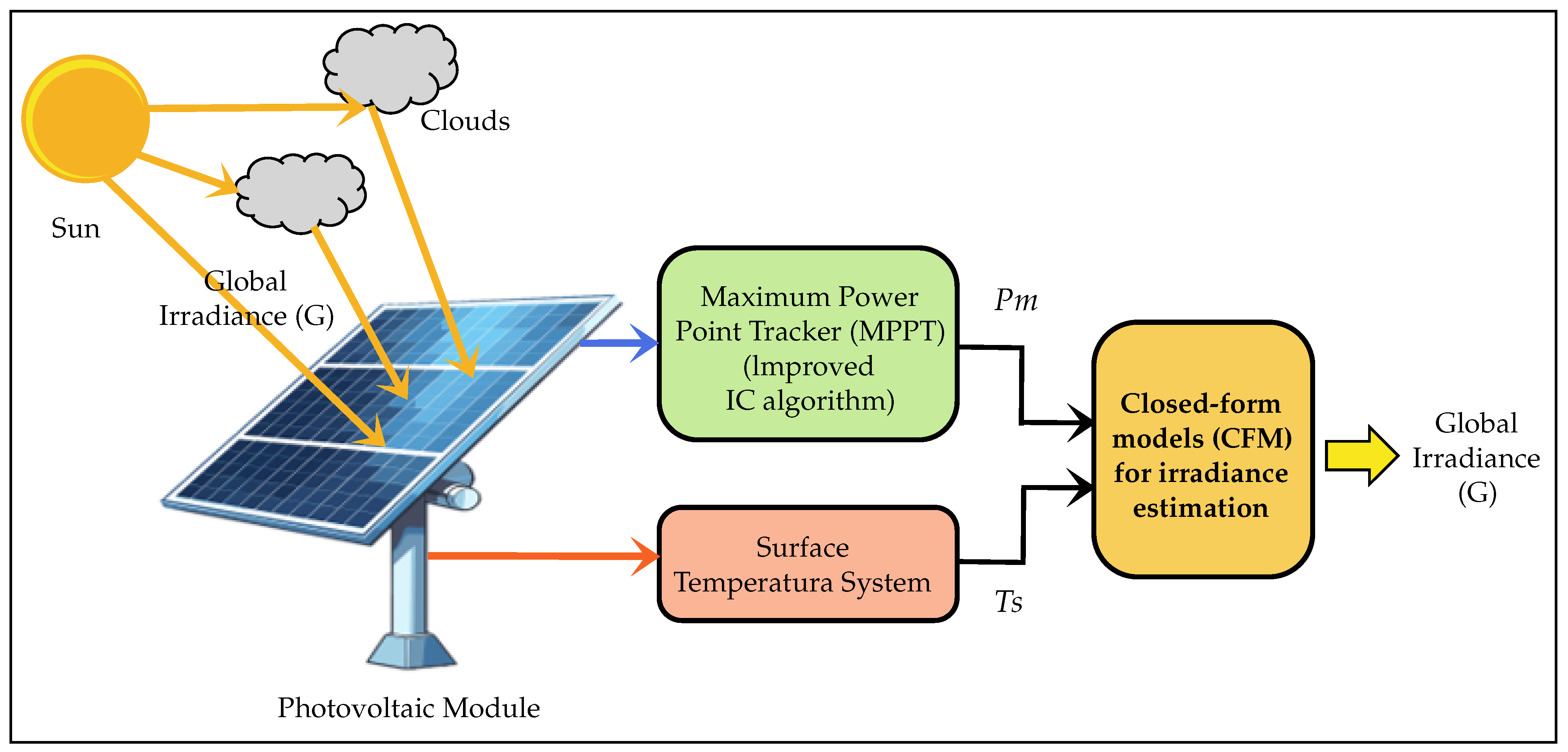
This section presents the design and implementation of the prototype, which in turn is composed of two systems, i.e., MPPT and the surface temperature system, developed in Section 2.1 and Section 2.2, respectively. The output of both systems provides the input variables, as shown in Figure 1, to the CFMs for irradiance estimation described in Section 2.3. The aim of the above systems is to collect the current and voltage at the point where the maximum generated power is extracted and the surface temperature of a PV module under clear, cloudy, or variable skies.
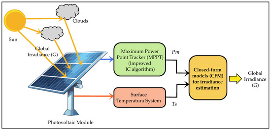
Figure 1.
System model.
Figure 2 presents a block diagram detailing the overall system’s operation, divided into three subsystems. The first subsystem corresponds to the MPPT system, controlled by an ATMEGA328P microcontroller (Manufacturer: Microchip Technology Inc.; City: Chandler; State: AZ; Country: USA), which is responsible for acquiring the current and voltage signals to adjust the duty cycle of the DC-DC converter using PWM signals. This control is carried out through a gate driver for MOSFET transistors. This microcontroller also collects the PV module’s surface temperature and the board’s temperature, which is designed to ventilate the switching circuits due to the heat generated by the continuous power dissipation at the converter’s final load. The second subsystem is a Davis Instruments weather station, model Vantage Pro 2 (Manufacturer: Davis Instruments Corporation; City: Hayward; State: CA; Country: USA), which provides global reference irradiance measurements obtained through its console’s USB serial port. Then, the data obtained by this subsystem and the data from the ATMEGA328P microcontroller are integrated into a central processing node. Finally, the third subsystem is the data logger, which is responsible for recording, storing, and analyzing irradiance estimates to evaluate the proposed system’s performance.
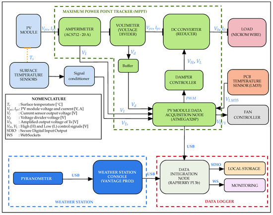
Figure 2.
Block diagram of the overall system’s operation.
On the other hand, the power curve of the PV modules is monotonic and does not present complex variations caused by partial shading, as the PV modules used have an effective area of approximately 0.5 m2, which minimizes the risk of partial shading significantly affecting the behavior of the system.
A summary of the notation we use in this article is shown in Table 1.

Table 1.
General notation.
2.1. MPPT Design
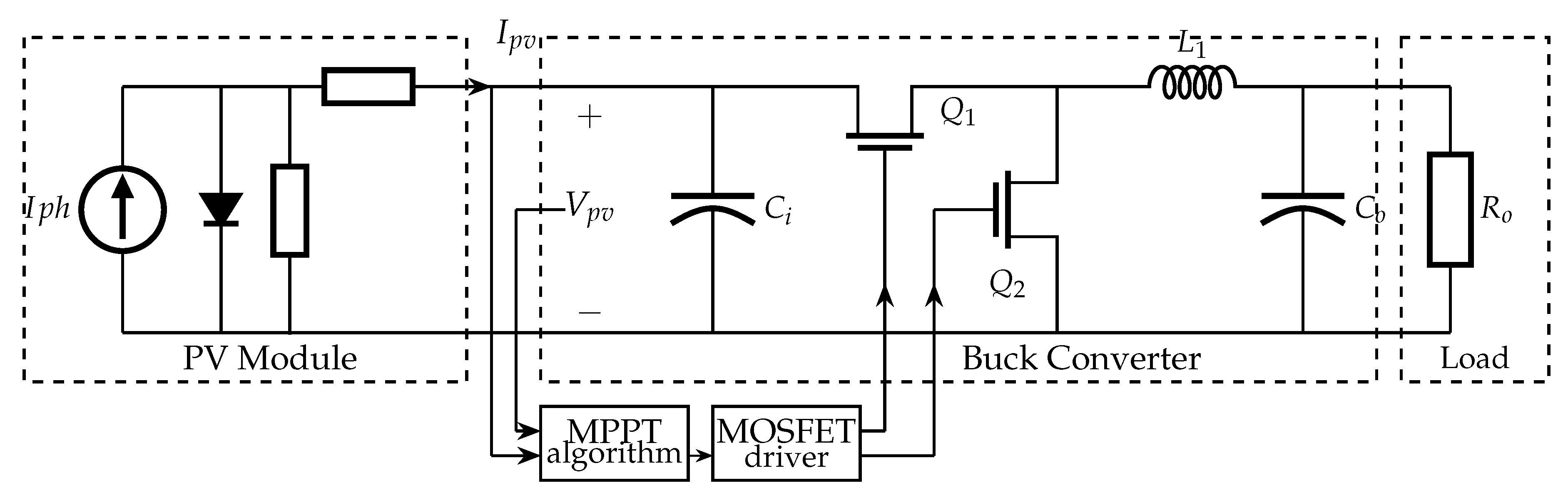
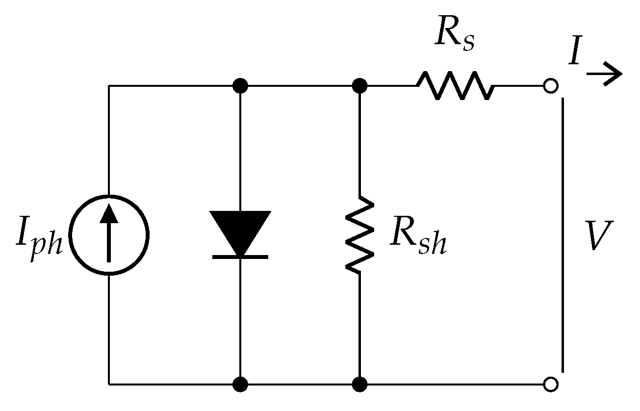
The MPPT system is composed of a DC-DC converter, an MPPT algorithm, and a controller for the MOSFET driver, as shown in Figure 3. The PV module is modeled by a single-diode equivalent circuit, which includes a current source, a shunt resistor, and a series resistor.

Figure 3.
MPPT based on a Buck converter.
2.1.1. Output Load Design
The selected DC converter is a Buck-type converter whose equation is a function of the input and output resistances and is expressed as follows:
where is the input resistance of the converter as seen from the PV module, which at the maximum power point (MPP) equals , which is the equivalent output resistance of the PV module at that point. The purpose of the converter is to track the MPP of the PV module by adjusting its duty cycle between [0, 1] [20].
Evaluating Equation (1) at the extreme values of D, the pairs (D, ): (1, ) and (0, ) are obtained. This analysis identifies the extreme operating points of the PV module. When increases to very large values, , the condition will depend on .
Table 2 shows the inverse relationship between irradiance (G) and . From this relationship and Equation (1), it is concluded that . Considering the minimum value of and its relationship with G, = 0.85 is selected for the maximum reference of G = 1000 W/m2, setting D = 1–0.85 for possible values higher than this reference. Therefore, solving Equation (1), it is obtained that .
Table 2.
Maximum operating points at STC and Nominal Operating Conditions (NOCs).
2.1.2. LC Filter Design
The value in Figure 3 is determined by Equation (2) based on [33], which is a widely known equation.
However, this equation does not consider a specific design procedure within an MPPT system, so the output voltage () and ripple current () must be substituted by the following expressions:
where is the maximum current through the output load. Equation (4) is based on [34].
where the scalar 0.3 is an intermediate value between efficiency and coil size. Therefore, replacing Equations (3) and (4) in Equation (2), we obtain the following:
Note that the inductance is now a function of a previously calculated value, and the duty cycle for the design under STC will be . Substituting the values for a switching frequency () of 55 KHz, we obtain that is equal to 27.31 H. The final inductance value was 100 H, achieved by winding an 18-gauge enameled wire around a toroidal core, which is higher than the critical value for both inductance and current to operate in continuous mode above 0.21 A.
The cut-off frequency of an LC filter is known to be:
The value of was chosen to be much smaller than , at least 100 times lower, with Hz. Substituting the values, we obtain C = 837 F.
2.1.3. Switching System Design
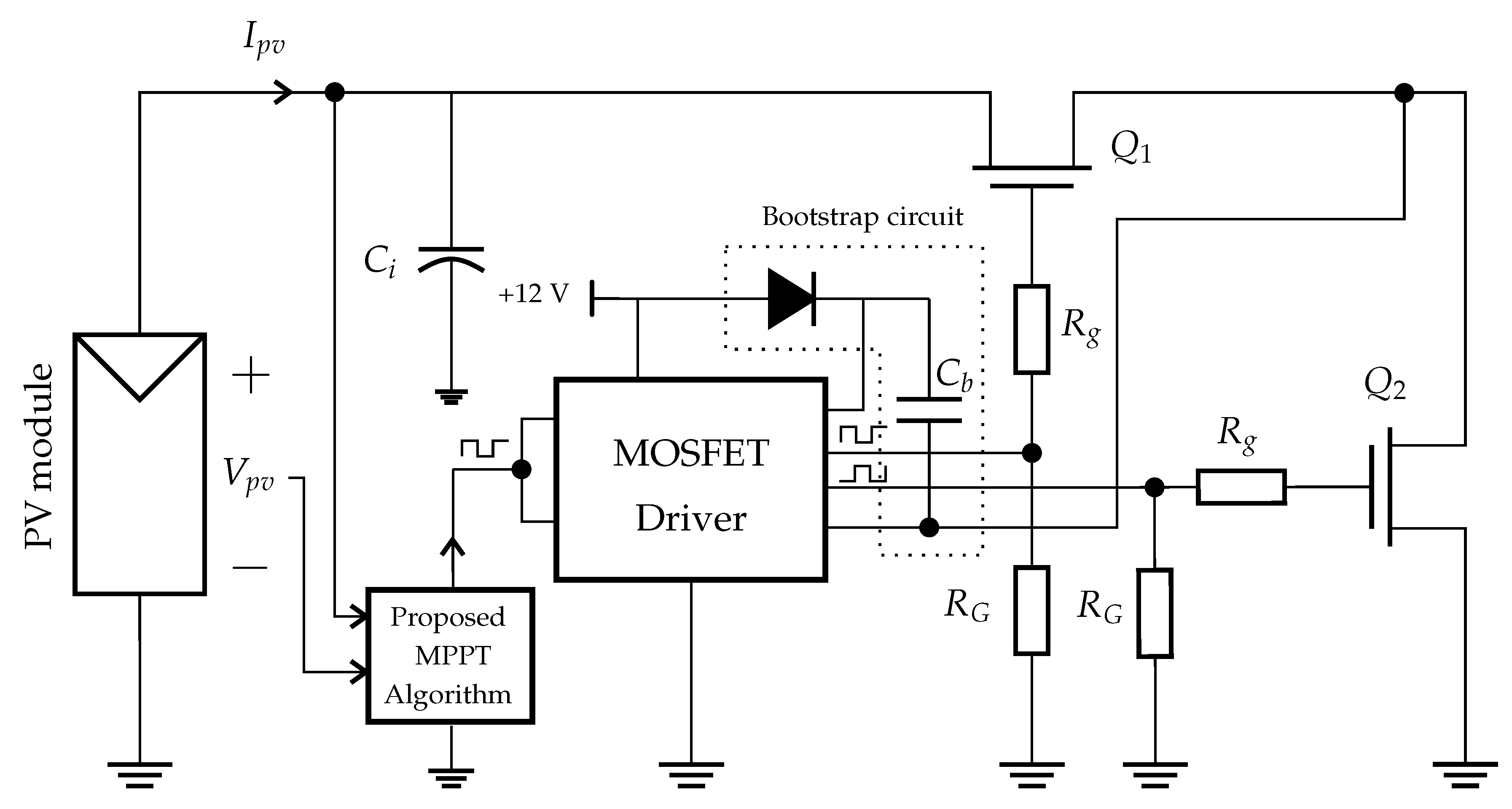
The switching system consists of a transistor bridge driver integrated circuit (MOSFET Driver), a Bootstrap circuit, a resistive impedance network for charging/discharging and also for limiting the source and bridge driver current, as well as the same power switching elements.
The MOSFET Driver will provide the necessary current to charge the internal capacitances of the MOSFETs through the charging and discharging of the Bootstrap capacitor, . Limiting this current to avoid damage to the integrated device and ensure a balance between the current required by the internal capacitances and the integrated circuit is necessary. The Gate series resistor, 36 , was obtained through testing and observation as a more reliable method before damaging the integrated circuit. The Gate resistor source, , will be needed to discharge these same capacitances previously described, for which a typical value of 10 KΩ can be used.
The Bootstrap capacitor is calculated in such a way that its value is [35]:
where is the capacitance present at the gate, and depending on the MOSFET, it can be calculated through:
The total gate charge, , for a voltage level is specified in the component datasheet. In this article, the IRF3205 MOSFET, whose is for V, is used. Based on this value, the optimum starting capacitor is determined to be . Figure 4 shows the circuit configuration with the MOSFET driver.

Figure 4.
Schematic circuit of the Buck converter switching system.
The controller used was the IR2103, which has two inputs and two pulse-width modulated (PWM) outputs, HIGH-side and LOW-side, 180° out of phase to achieve synchronous switching. The inputs were short-circuited because the converter will operate continuously for most of the day without considering the discontinuous mode, corresponding to atmospheric time periods such as sunrise and sunset. Comparisons with the reference instrument or pyranometer show that the PV module exhibits different cosine responses, considering that the experiments will be conducted on a horizontal plane.
In summary, the most relevant parameters of the DC-DC Buck converter for the MPPT are detailed in Table 3.
Table 3.
Parameters of the designed converter.
2.1.4. Proposed MPPT Algorithm
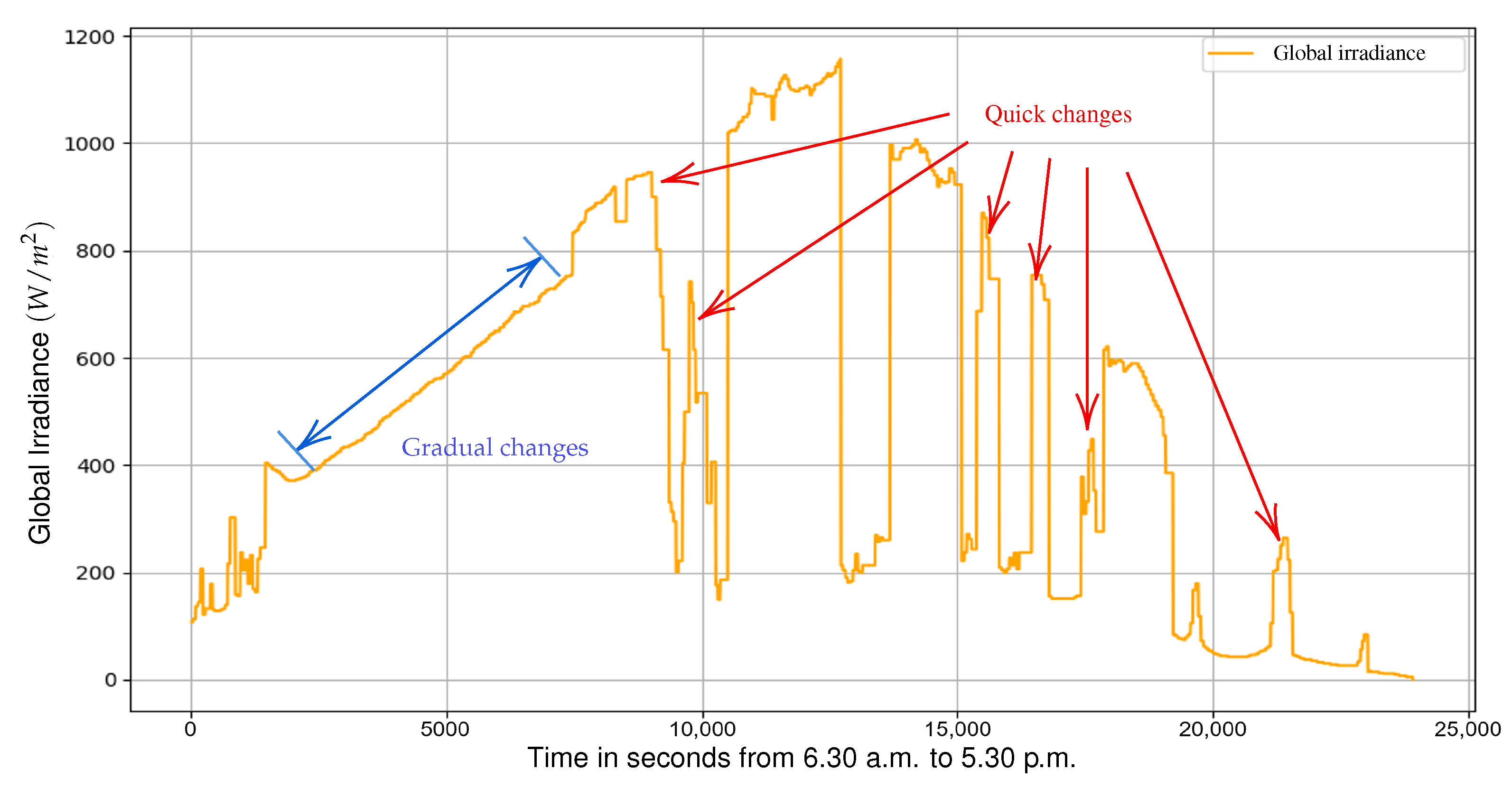
For the current and voltage feedback, as shown in Figure 4, an ACS712-20A module and a voltage divider were used, respectively. Both were calibrated and compared with a Fluke 287 multimeter, with a large set of data collected in parallel to ensure the reliability of the MPP measurements and, consequently, guarantee the proper functioning of the proposed algorithm. The proposed algorithm incorporates an additional implementation in which the step size () dynamically varies from a higher value to a lower one, progressively over time intervals in seconds, on top of the IC algorithm. Two changes in irradiance levels due to the speed of cloud movement in the atmospheric sky have been identified: gradual and rapid changes, as shown in Figure 5. Due to this, a detector is implemented that measures the magnitude of the changes in terms of power, voltage, and current variations, which are integrated into a single variable. Likewise, the MPPT IC algorithm proposed is based on [20]. It does not include MPPT under partial shading conditions because the adequate area dimensions of the PV modules are relatively small, approximately 0.5 m2.

Figure 5.
Identification of gradual and quick changes in the irradiance pattern for a typical day in the city of Cusco.
This relationship is expressed by the following equation from [36]:
where M is power change detection variable. This equation is derived by approximating and in the equation for the derivative of power with respect to voltage at the maximum power point () [37]:
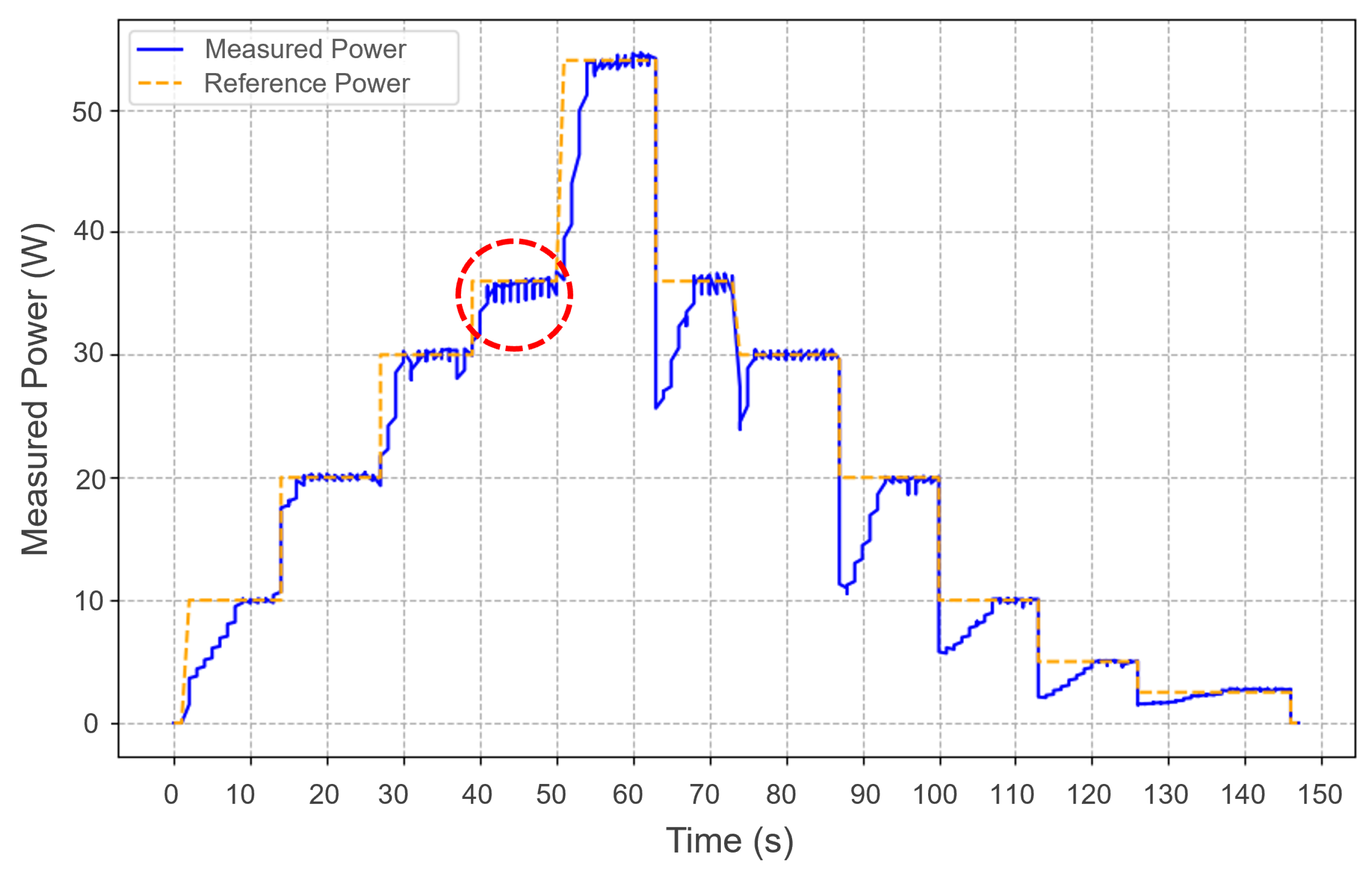
The IC algorithm has been implemented, demonstrating that it satisfactorily follows the assigned power levels, as shown in Figure 6.
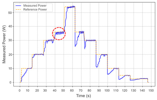
Figure 6.
Performance of the IC algorithm for different power levels.
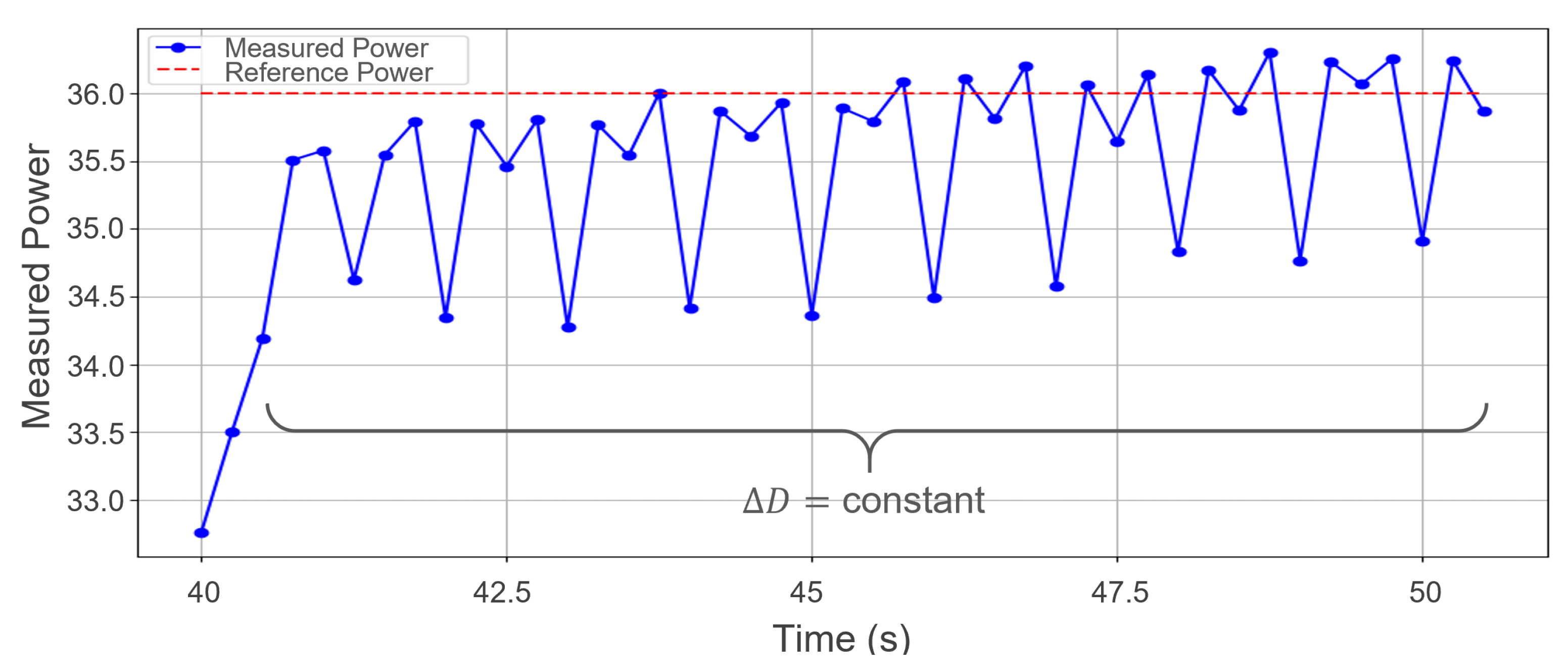
The typical oscillations of this IC algorithm are observed in Figure 7 for a period between 40 and 50 s at 36 W input power reference from Figure 6 (red circle) for a constant . Therefore, to control and stabilize these oscillations, the millis() function of Arduino was used to assign different values of with a total duration shorter than the time it takes for the traditional IC algorithm to reach the MPP. In this case, the Arduino microcontroller achieved this within 4 to 5 s.
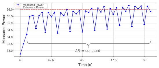
Figure 7.
Oscillations observed at the maximum power point for 36 W input power.
Using a Tektronix PWS4305 30 V/5 A power supply (Manufacturer: Tektronix, Inc.; City: Beaverton; State: OR; Country: USA), it was possible to emulate the rapid changes in irradiance described earlier but not the gradual changes due to the power supply’s limitations and the impossibility of comparing real and reference values. As a result, the following values of were obtained, as shown in Table 4. The values of this last variable are presented in an 8-bit unsigned integer format.
Table 4.
Values of M and for smooth and abrupt changes in irradiance.
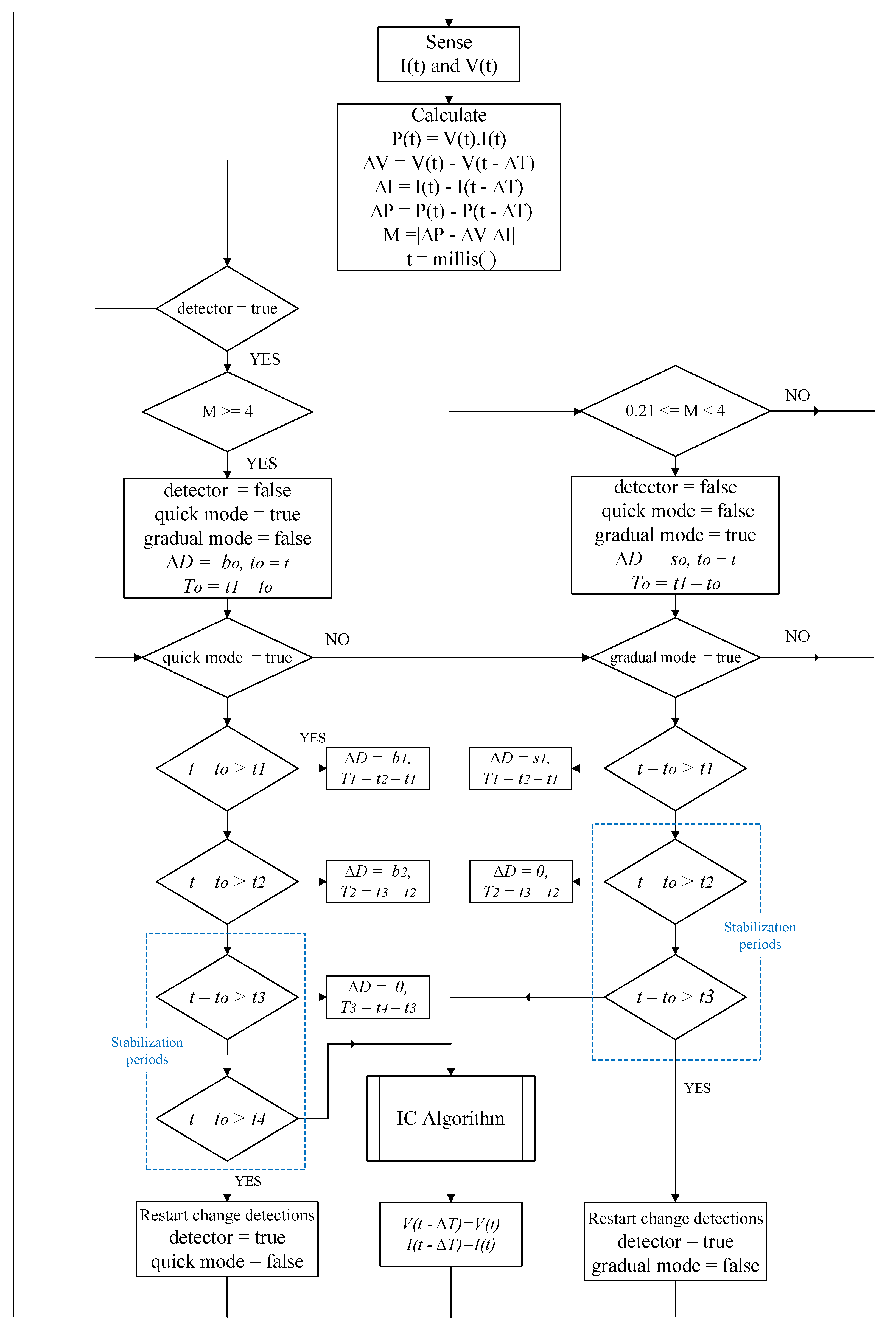
Likewise, Table 4 specifies the respective duration of each . The sequence of these values is described by and , representing the values for smooth changes (s) and abrupt changes (b), ending at to stabilize the MPP. This procedure is shown in the flowchart in Figure 8, which details the operation of the proposed algorithm. A detailed description of its operation follows.
- Sense and calculate electrical variables: In the first instance, the current (I) and voltage (V) are measured to calculate the power (P) and the variations of V, I, P, and M. At the program startup, the voltage and current are initialized to zero. Next, the execution time of the program up to that moment is stored in an unsigned long variable, . Additionally, is initialized to zero.
- Enable change detection: If the value of M is greater than or equal to 4, the program disables the detection of further changes as well as the action of modifying the step width for smooth changes, described by gradual mode. If the value of M falls within [0.21, 4], it also disables change detection, but, this time, deactivates quick mode.
- Execution of the IC algorithm in parallel to changes in : When the detected change is “gradual mode”, for 1 s, then for 2 s, and finally to stabilize the maximum power point. Similarly, when the change is “quick mode”, will this time start at and continue progressively to , ending at . During this value assignment, the IC algorithm runs in parallel, which is made possible by the function millis().
- Restart change detection: Once is reached, another short period of time is allotted to ensure that the oscillations stabilize. The program then re-enables change detection for the next search until the set thresholds are exceeded.
The flow diagram in Figure 8 shows that the duration of the step widths is expressed in terms of time instants. This is because the value of t is updated in each iteration of the program loop and must, therefore, be compared with the values of , , , and . This logic is applied when executing , , , and , .
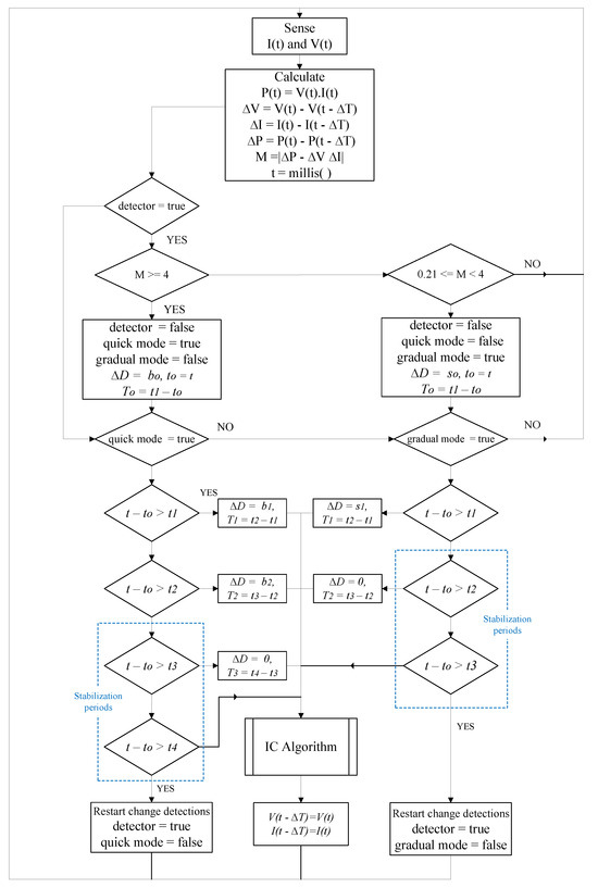
Figure 8.
Flowchart of the proposed improved IC algorithm for eliminating oscillations and controlling sensitivity in irradiance changes.
Figure 8.
Flowchart of the proposed improved IC algorithm for eliminating oscillations and controlling sensitivity in irradiance changes.
2.2. Surface Temperature System Design
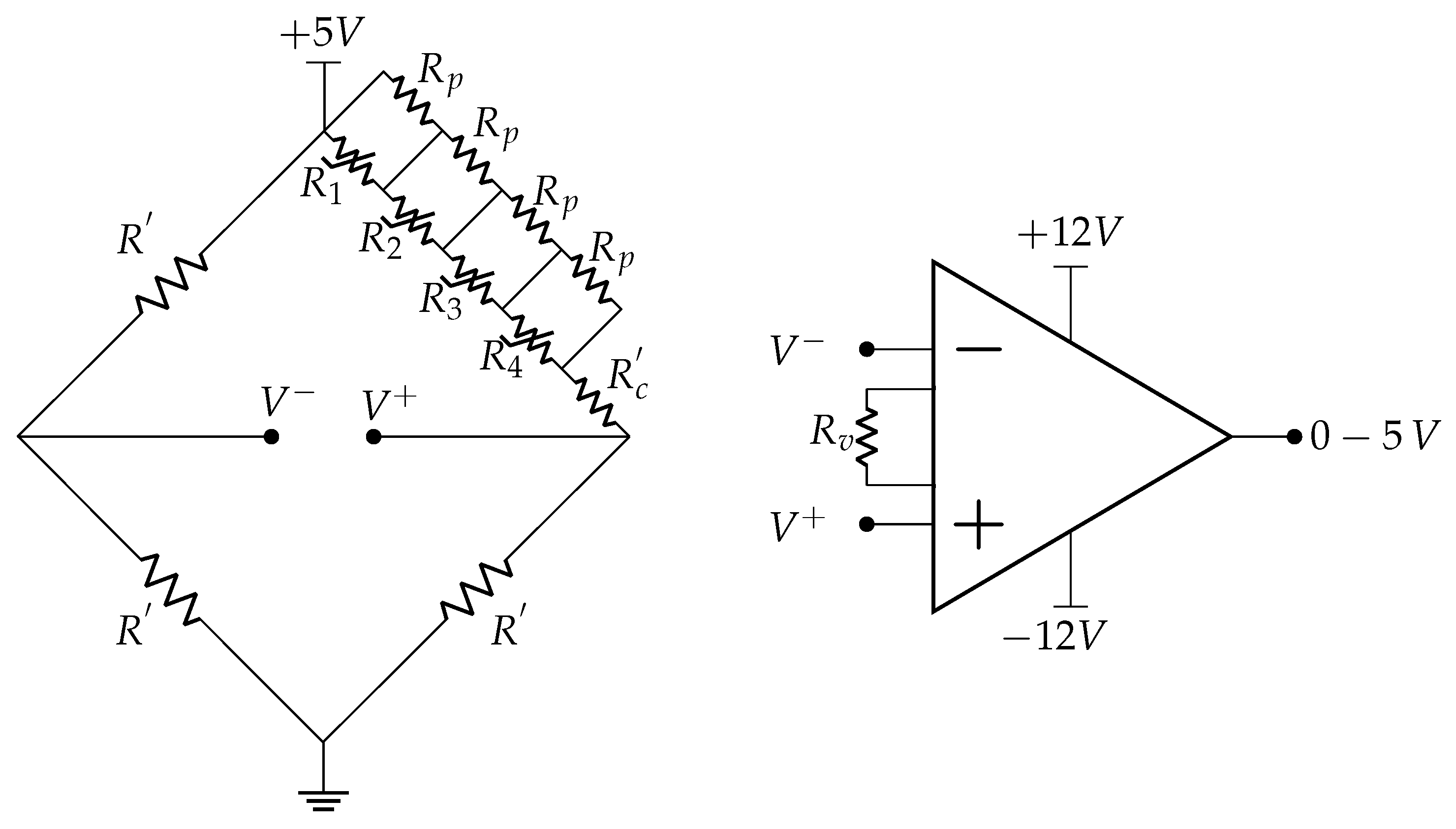
Due to the temperature variability on the PV module’s surface, an average temperature measurement system was designed using four NTCs located at strategic points. These NTCs are connected to a single instrumentation amplifier to optimize data acquisition. The system design is similar to that of a single NTC within the temperature range of 18 °C to 86 °C. Based on this model, the value of the linearization resistor, , connected in parallel to the NTCs, is determined as shown in Figure 9.

Figure 9.
Wheatstone bridge with 4 NTCs for surface temperature measurement of a PV module.
The resistance value at the average temperature for the TTF series NTC thermistors is as follows:
The value of the bridge resistors is equal to the variation of the fixed thermistor-resistor array (–) over the entire indicated temperature range (18 °C an 86 °C) multiplied by 100 to amplify the resolution of the bridge output voltage given by:
where , and in turn, and , and is the linearized thermistor or in parallel with .
Finally, the last element on the same branch of the circuit as the thermistor is a compensation and reference resistor, which ensures that the voltage difference at the output of the bridge is zero when °C.
Based on above, the voltage difference at the bridge output considering a single thermistor is as follows:
Now, considering four thermistors, and change in value as three additional thermistors are added in series with their respective resistors in parallel. Therefore, we have the following.
However, since all thermistors are of the same type, it is stated that:
With Equations (18) and (19), the expressions for and in Figure 9 are obtained as functions of Equations (12) and (13).
Equation (21) describes the voltage difference at the output of the bridge in Figure 9, considering the four thermistors.
where is the sum of the linearized NTC thermistors, expressed as , and arranged in series. Note that Equations (14) and (21) differ only in the term , corresponding to the average value of the four thermistors, which can be found at different temperatures. Therefore, the voltage difference obtained represents the average temperature measured by the thermistors. The parameter values, , , , and , of the designed Wheatstone bridge, developed and determined previously, are summarized in Table 5.
Table 5.
Parameters of the designed Wheatstone bridge.
2.3. CFMs for Irradiance Estimation
2.3.1. Osterwald’s Model
The model is based on understanding how a PV module responds under non-standard conditions, which differs from STCs. This approach allows for the efficiency of the PV module to be compared, taking into account factors such as device temperature and total incident irradiance level. Adjusting the measurements according to the specific conditions during the test allows the performance of the PV module to be evaluated in a real operating environment and not only under ideal conditions. According to [11,19], the maximum power as a function of irradiance and temperature using values given by the manufacturers is:
Solving for G, the irradiance estimation model is obtained as a function of the maximum generated power, the temperature of the PV module, and some parameters provided in the manufacturers’ data sheets.
where is the maximum power under STCs, is the global irradiance at STC, equal to 1000 W/m2, is the normalized temperature coefficient of maximum power (%/°C), is the temperature of the PV module (°C), is the PV module temperature at STC, equal to 25 °C, and is the PV module efficiency under STCs.
2.3.2. Model According to IEC 60891 Standard
This model follows a principle similar to that of the Osterwald model, designed to adjust PV module measurements obtained under real conditions to compare them with performance under STC. The main difference is that this model evaluates how current and voltage vary regarding their maximum current and voltage values under STC.
Furthermore, it is important to note that the model based on IEC 60891 assumes operating conditions close to the MPP and makes use of parameters obtained at STC, such as short-circuit current, open-circuit voltage, and nominal temperatures. It also considers the absence of partial shading, which is feasible in small systems with good solar exposure. This approach also assumes that the PV module has not undergone severe degradation, so that an ageing correction may be required for older PV modules.
The operating point V-I of a PV module can be calculated based on [12,14,18] with the expression following:
where and , is the current in the MPP, is the voltage in the MPP, is the short-circuit current under STC, is the open-circuit voltage under STC, is the relative temperature coefficient of short-circuit current (A/°C), is the relative temperature coefficient of open-circuit voltage (V/°C), is the global irradiance at STC, equal to 1000 W/m2, is the temperature of the PV module, is the PV module temperature at STC, equal to 25 °C, and is the series resistance of a PV cell.
Solving Equations (24) and (25) simultaneously, and after isolating and rearranging G, gives the global irradiance estimate, , shown as follows.
Note that Equation (26) does not depend on temperature but rather on the series output resistance, , according to the single-diode, five-parameter model. Based on [13], is the same as the output resistance under STC, , and can be approximated according to [38] as:
2.3.3. Model Based on the Characterization of a PV Cell
This estimation model is based on Equation (28), which represents the characteristic equation of curve V-I of the simplified equivalent circuit of a PV cell with four parameters. However, this simplified model does not take into account the parallel or shunt resistance in Figure 10 given by [13].
where is the thermal voltage and is the photogenerated current of the PV module.

Figure 10.
Simplified model of the PV module.
In Equation (28), the PV module’s output voltage depends on the photogenerated current () and the open-circuit voltage (), which in turn are functions of G and cell temperature. Therefore, the equations for these variables are defined as follows [11].
For the short-circuit current:
For the open-circuit voltage:
Considering that and , is based on [13] and given by:
3. Results
This section presents the main numerical results based on the models described above. Numerous tests were performed to obtain the results, including two measurement types. Firstly, laboratory tests were performed to validate the performance of the implemented circuits. Secondly, tests were performed under real conditions, i.e., field tests to compare the G measurements with the estimates obtained from the CFMs.
For the tests of the converter input power and equivalent load resistance, a duty cycle sweep was performed from approximately 15% to 95%, considering an input voltage of 18.5 V and a current of 4.35 A, values corresponding to the STCs of the PV module used, as shown in Table 2. On the other hand, to evaluate the performance of the proposed improved MPPT IC algorithm, the MPPT algorithm was tested on the implemented converter, using the same power supply to show the performance of the IC algorithm in Figure 6. For this purpose, successive stepped power levels of 2.5, 5, 10, 12.5, 17.5, 35, 47, 70, and 80.5 W were assigned in ascending and descending order until the maximum reference power under the STCs was reached. To evaluate the final objective of this article, which is the closed-form models, an additional PV module of the same characteristics as the one already installed with 10 years of service at the institutional laboratory TESLA of the Universidad Nacional San Antonio Abad del Cusco (UNSAAC) was installed. The installation of the PV module is described and shown in Section 3.3. On the other hand, the evaluation of the models is performed using two accuracy metrics: the mean absolute percentage error (MAPE) and the root mean square percentage error (RMSPE) [31,32]. The parameter values used in this article are based on the technical characteristics of the PV modules used [39], shown in Table 6.
Table 6.
PV module parameters.
Finally, the hardware, software, and tools used for the tests at the laboratory level and in real conditions are as follows. A Raspberry Pi 3 model B (Manufacturer: Raspberry Pi Foundation; City: Cambridge; Country: UK) which has as hardware a Broadcom BCM2387 chipset and a quad-core ARM Cortex-A53 processor. An Arduino Nano microcontroller (Manufacturer: Arduino; City: Ivrea; Country: Italy), with dimensions of 45 mm × 18 mm, based on the ATmega328P 8-bit microcontroller, 16 MHz clock frequency, 32 KB Flash memory, 2 KB RAM, 1 KB EEPROM, and communication via UART, SPI, and I2C. As a reference instrument for comparing irradiance estimates, a pyranometer SKU6450 (Manufacturer: Davis Instruments; City: Hayward, CA; Country: USA) was used, based on a silicon photodiode with a spectral response between 400 and 1100 nanometers, 1 W/m2 of resolution, 0 to 1800 W/m2 of range, of accuracy (Reference: Eppley PSP at 1000 W/m2), and an update interval of 50 to 60 s. Programmable DC power supplies Tektronix PWS4305 (Manufacturer: Tektronix, Inc.; City: Beaverton, OR; Country: USA), Linear Regulation, up to 30 V Output Voltage, up to 5 A output current, 0.03% Basic Voltage Accuracy, 0.05% Basic Current Accuracy, less than 5 Ripple and Noise.
3.1. MPPT System
3.1.1. Converter Performance
Figure 11 shows the converter input power and equivalent load resistance as a function of the converter duty cycle. We can see that the maximum power point is reached with a duty cycle of 80%, which is close to the design value. Also, we can observe the curve of the equivalent load resistance (green line) at the input of the converter, as seen from the power supply, whose shape is consistent with the hyperbolic function of Equation (1). The blue line shows the input power seen from the power supply, which increases until it reaches approximately the programmed power value of 80.5 W, after which it decreases. In relation to the equivalent resistance, it is observed that the maximum power value is obtained at a resistance of which is very close to the value in STC conditions in Table 2. On the other hand, the calculated efficiency of the converter is 94%, which shows a high system performance.
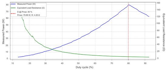
Figure 11.
Load conditions and maximum achieved power close to the reference design duty cycle.
3.1.2. Performance of the Proposed MPPT IC Algorithm
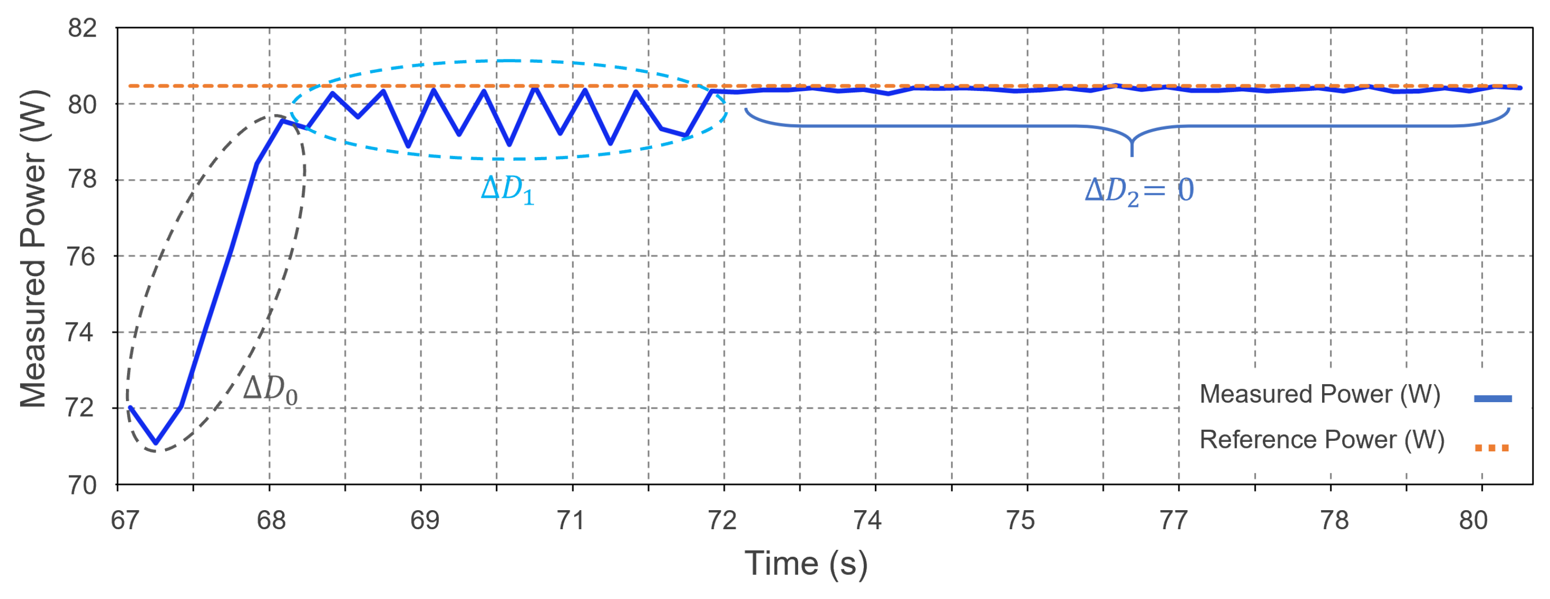
In Figure 12, we can observe the performance of the proposed IC algorithm under different input reference power levels. Unlike the traditional IC algorithm, the proposed algorithm eliminates the oscillations that appear at the maximum power point in Figure 7, which can be better appreciated by analyzing the performance of the improved algorithm, for example, for the reference level of 80.5 W in the time range of 67 to 82 s from Figure 12 (red circle) in Figure 13. The latter figure shows the change of the duty cycle step widths, , reflected in the variation of the amplitudes of the oscillations around the MPP until they are eliminated with equal to zero.
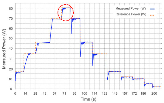
Figure 12.
Improved IC algorithm performance for different power levels.
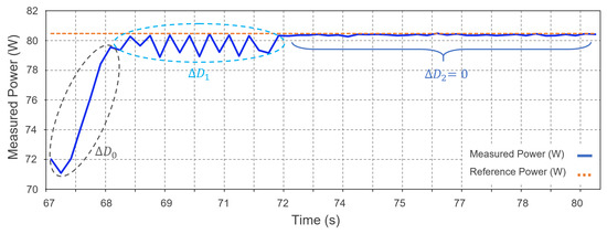
Figure 13.
Improved MPPT system response for 80.5 W input power.
Table 7 presents the results of the evaluation of the metrics to determine the performance of the proposed IC algorithm. The calculated mean absolute error (MAE) is 0.2 W, which reflects a high accuracy in MPP tracking and an efficiency of 99.88%, indicating a maximum utilization of the input power. The convergence time varies between 3 and 5 s, which shows the algorithm’s speed in reaching the MPP.
Table 7.
Evaluation metrics for the improved MPPT IC algorithm.
3.2. Temperature Measurement System Test
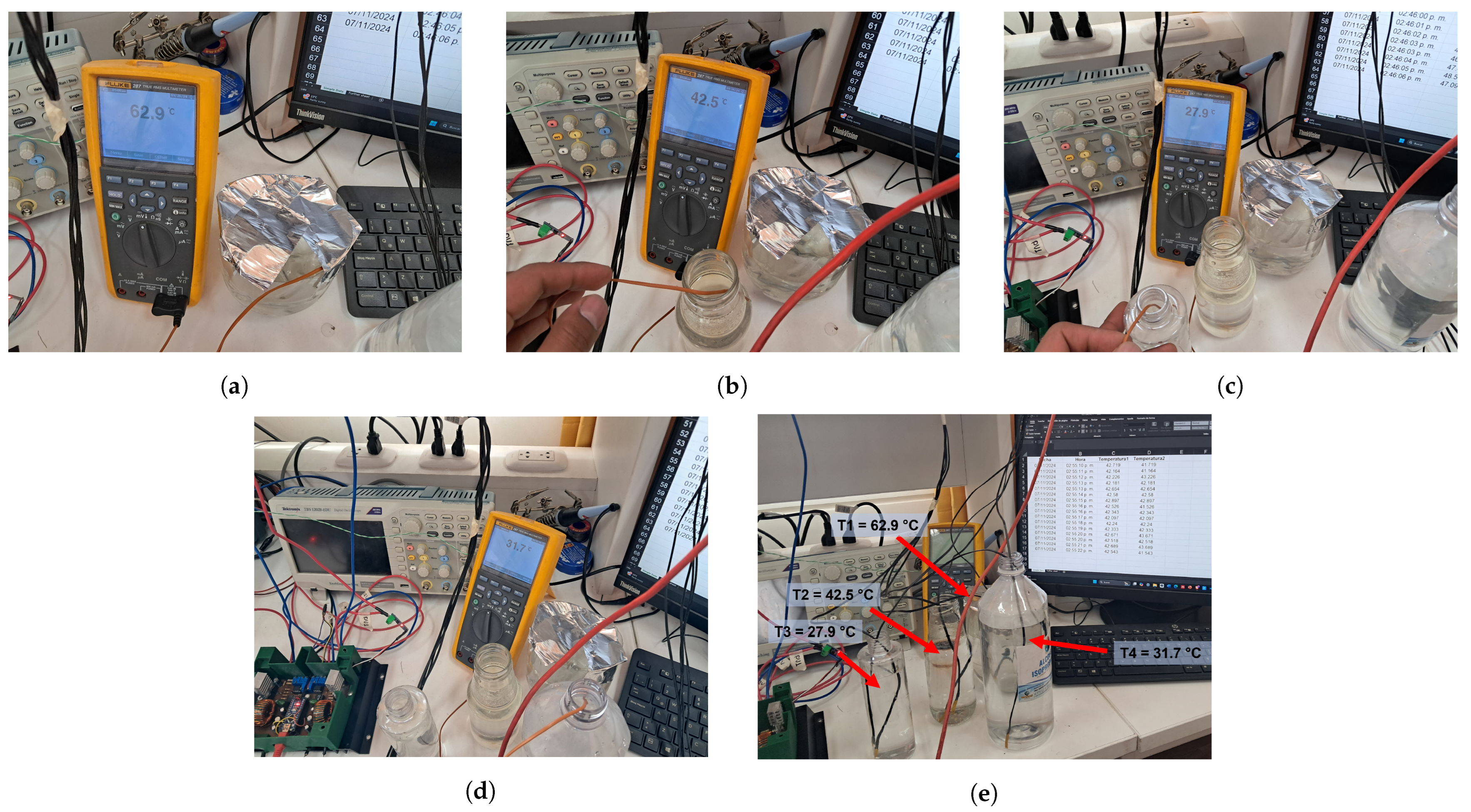
Figure 14 shows the verification of the temperature measurement system. Four plastic containers with water at different temperatures were used, as shown in Figure 14a–d. So, the system calculates the final temperature as the average of the measurements in these four containers. Therefore, the results of measuring the temperatures in these vessels with the K-type thermocouple coupled to a Fluke 287 multimeter demonstrate the system’s accuracy. The results confirm the correct functioning of the averaging system, as the final reading recorded by the system was 41.25 °C. Finally, Figure 14e shows the values recorded by the system, which vary between 41 °C and 42.5 °C, validating the accuracy of the average temperature estimation.

Figure 14.
Temperature measurement of water tanks is used to test the temperature averaging system. (a) = 62.9 °C, (b) = 42.5 °C, (c) = 27.9 °C, (d) = 31.7 °C, (e) testing of the averaged system.
Figure 15 shows the evaluation of the measurement system by means of a temperature sweep from 20 to 63 °C, using four thermistors immersed in the same water tank. The results show a variability of ±2 °C in the readings, while the correlation with the reference values reaches a coefficient of 0.9974, indicating a strong relationship between the two measurements. This test establishes the correlation between the thermistor readings and the reference values and analyzes the variability of the measurements using a histogram.
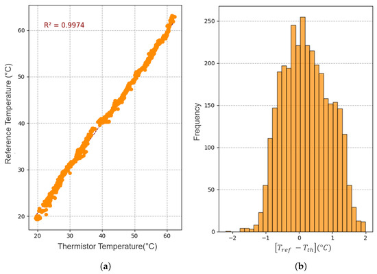
Figure 15.
Comparison of pairs of data between thermistor array readings and reference thermometer. (a) Scatter plot in the range 20 °C to 60 °C. (b) Histogram of the differences between the reference and thermistor readings.
3.3. Evaluation of Closed-Form Models
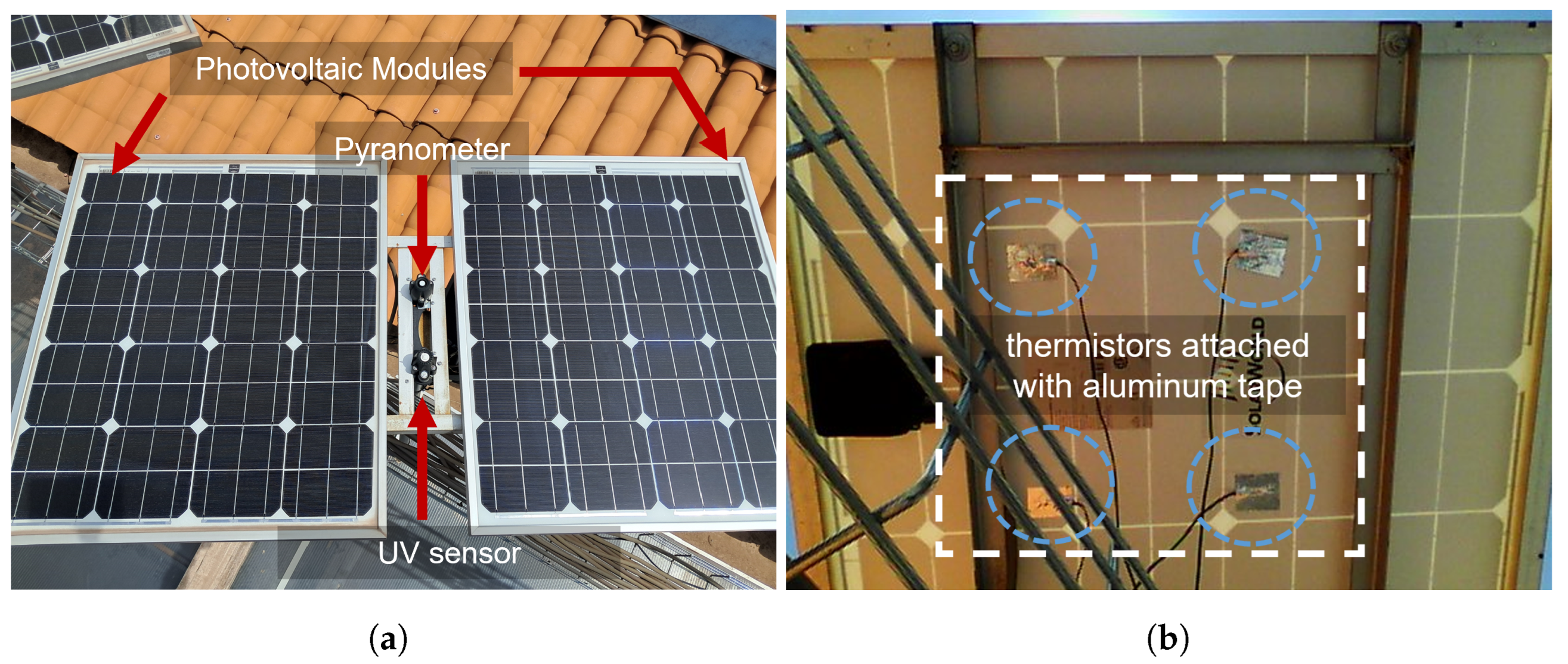
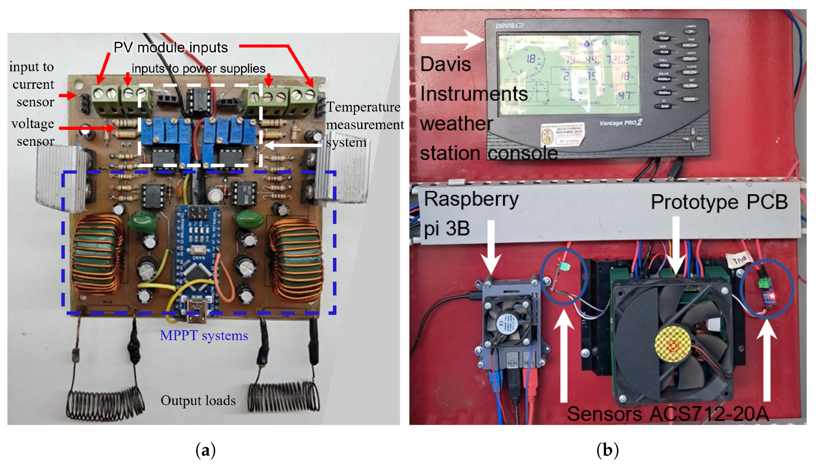
Figure 16a shows the installation of an additional PV module aligned in the same tilt plane as the Davis Instruments pyranometer. Figure 16b shows the placement of the thermistors on the back of the modules with aluminum tape to have a good approximation of the internal temperature of the modules based on [40]. On the other hand, Figure 17a shows the implementation of the designed circuits, including the MPPT system and the temperature measurement system, on a single double-layer PCB board. Figure 17b shows the prototype installed inside a cabinet together with the other elements necessary for data acquisition and acquisition.

Figure 16.
Equipment installed and implemented. (a) PV modules are installed on the same plane as the pyranometer. (b) Thermistors fixed with aluminum tape on the back of the PV modules.
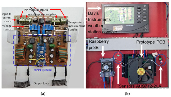
Figure 17.
Prototype implemented and installed. (a) A PCB circuit was implemented to measure the maximum power and surface temperature in real time. (b) Prototype installed inside a cabinet for data acquisition.
Independent of the data integration node, the system pyranometer, and the temperature measurement system, the maximum power tracker is powered by 5 V with a total current of 32 mA.
This configuration allows the simultaneous collection of data from a PV module that has been used for several years and from a newly installed one. On the other hand, the data were collected through a Raspberry Pi 3B, which integrates and synchronizes the information from the Arduino Nano microcontroller and the Davis Instruments Vantage Pro2 Weather Station console. In addition, communication with both devices is performed through USB connections, using Node-RED for the management and local storage of the information, with a sampling rate of 7 s.
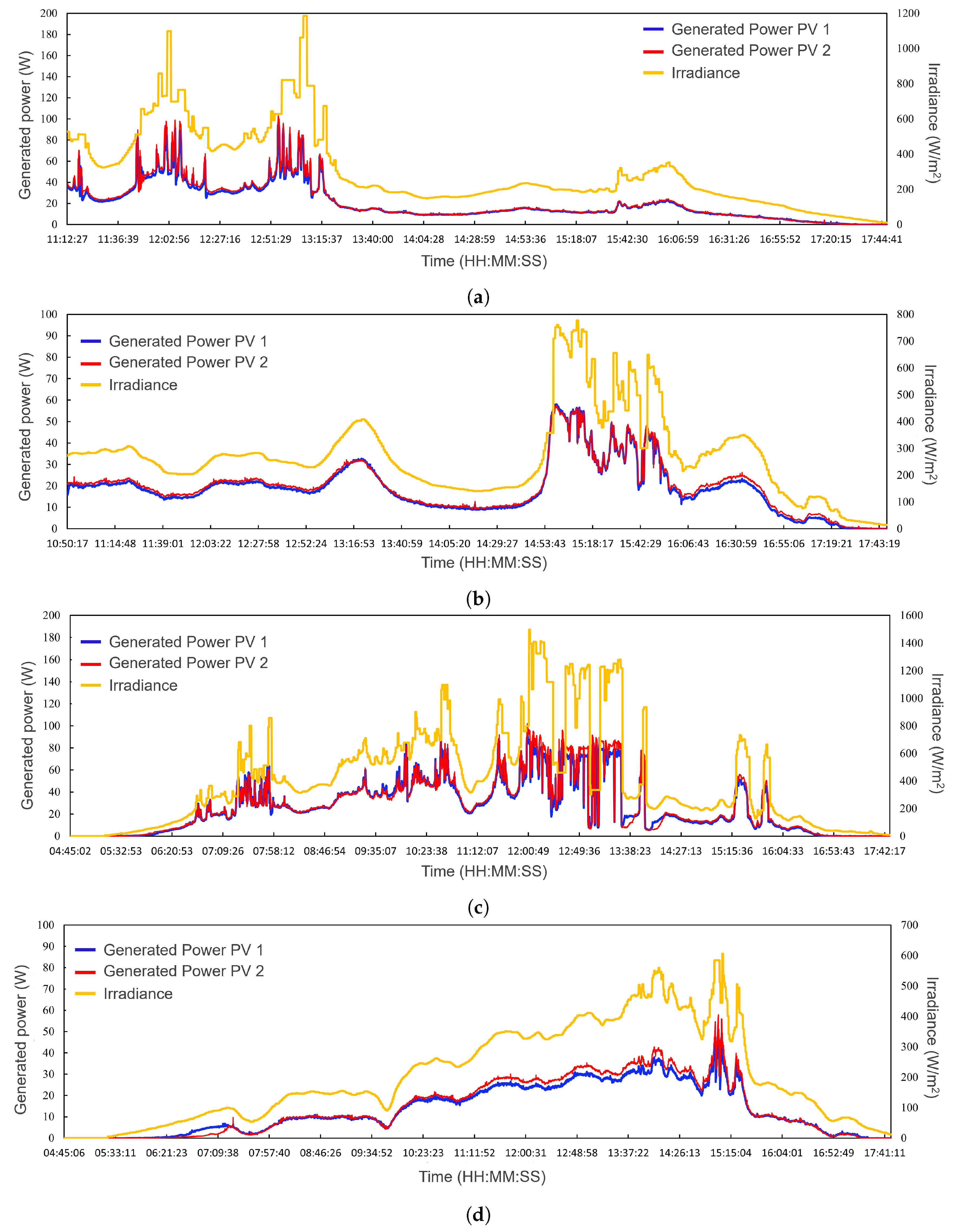
Figure 18a,b,d show the weather conditions with rapidly varying cloud cover. Figure 18c shows the fast irradiance variations due to the large amount of irradiance peaks. The data were collected over 4 days in mostly cloudy conditions, from 20 to 23 November 2024. The yellow line represents the reference irradiance, while the blue and red lines show the power of PV modules 1 (used) and 2 (new), respectively, following a similar pattern, indicating the correct functioning of the power trackers. However, the pyranometer presents a limitation in its response time (50–60 s), which has generated disagreement with the measured power; this can be clearly seen between noon and 13:00 h in Figure 18a.
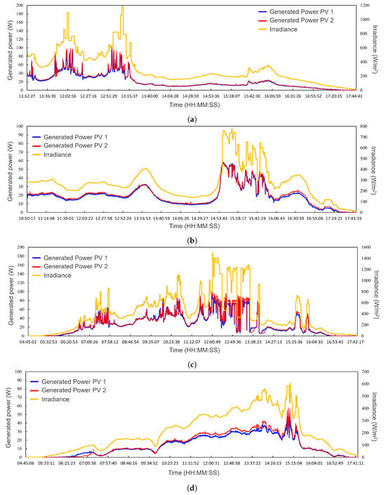
Figure 18.
The pattern of maximum irradiance and power generated by the PV modules. (a) Profiles of 20 November—day 1. (b) Profiles of 21 November—day 2. (c) Profiles of 22 November—day 3. (d) Profiles of 23 November—day 4.
On the other hand, the models were applied with the following consideration: the series resistance of the circuit model, obtained using Equation (27), was ,
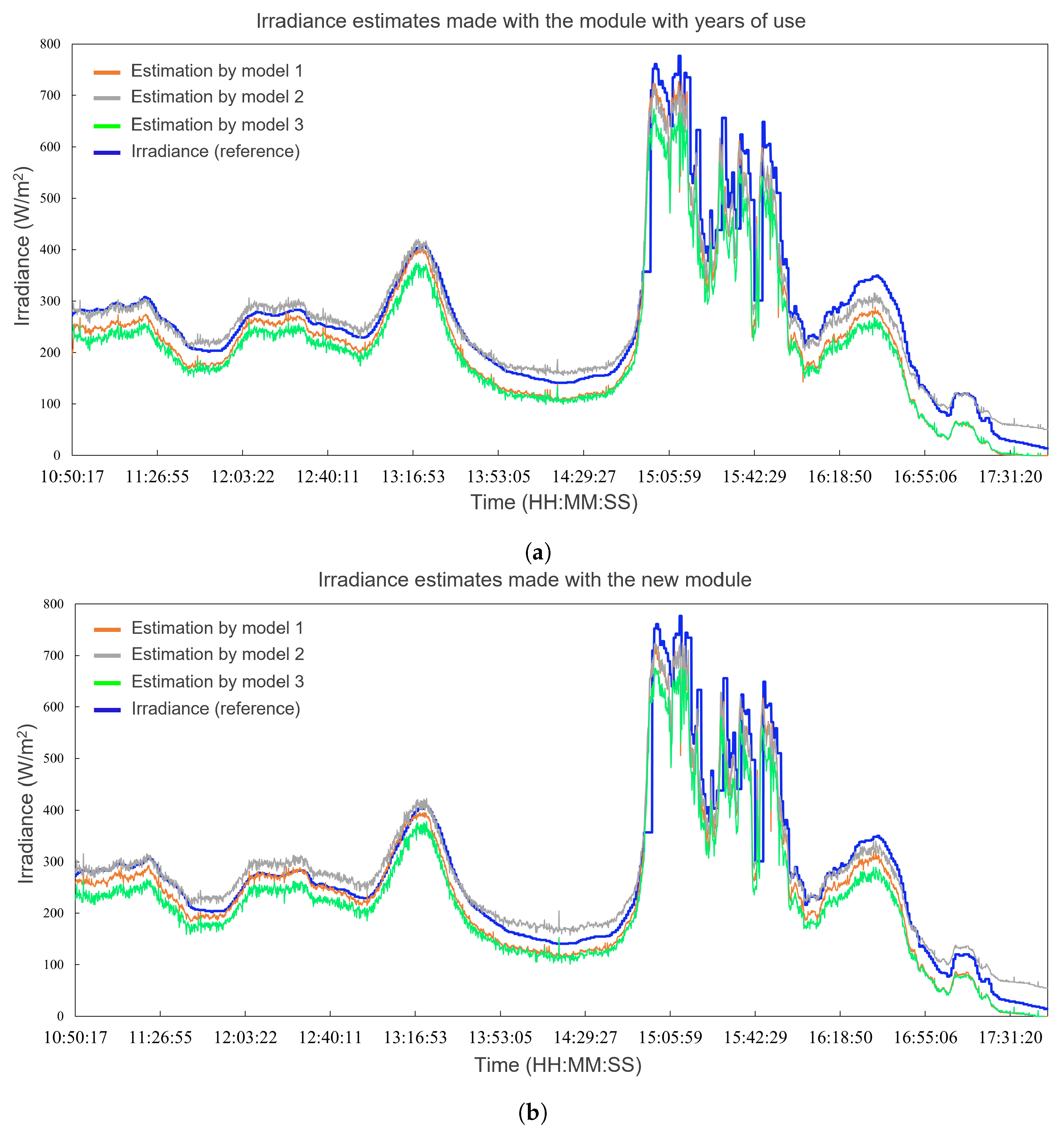
Based on the above, Figure 19 shows the approximation of the estimates to the reference (blue line).
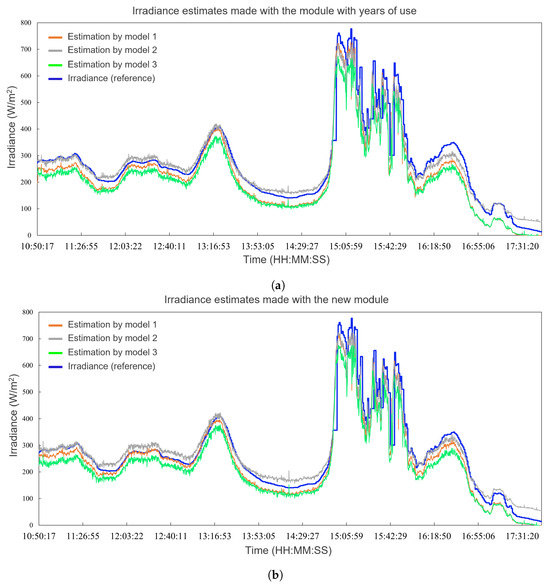
Figure 19.
Comparison between the estimates using the CFMs and the pyranometer sensing. (a) Comparison in the PV module with years of use. (b) Comparison in the new PV module.
The models were evaluated by calculating two metrics: MAPE and RMSPE [31,32]. The main difference between the two lies in how they treat deviations of the estimates from the true value measured by the pyranometer. While the MAPE measures the mean error in absolute terms, the RMSPE gives greater weight to significant errors, penalizing them more heavily. The mathematical expressions for MAPE and RMSPE are analogous to [19]. These metrics are presented below.
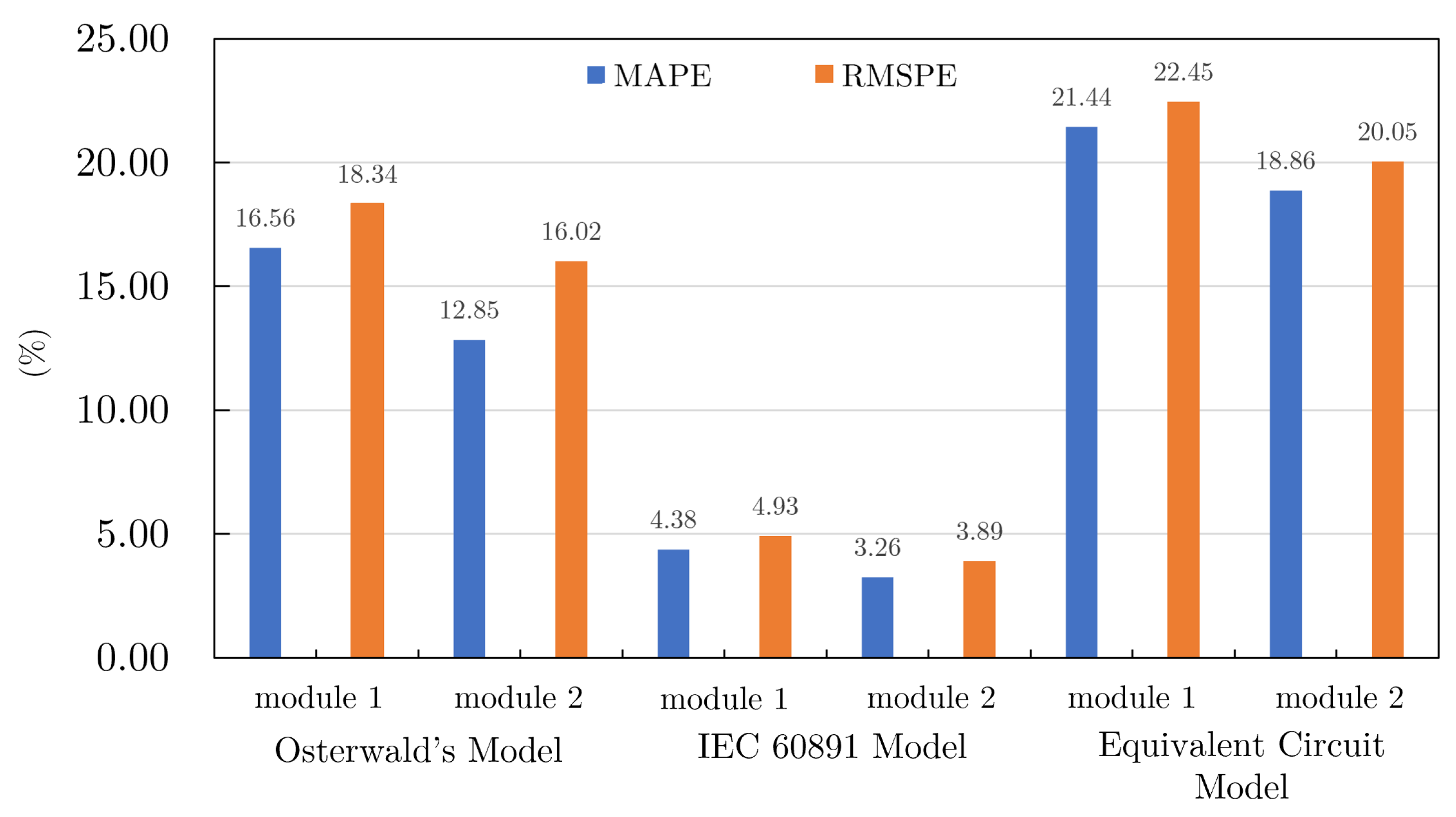
On the other hand, Figure 20 shows the results of the MAPE and RMSPE calculations for each model and photovoltaic (PV) module. Furthermore, the model is based on the IEC equations, showing the highest accuracy (errors < 5%), while the equivalent circuit model presents the highest uncertainty (errors > 20%), followed by the Osterwald model. We can also observe that the estimates are more accurate for module 2 (new) than module 1 (used), suggesting degradation due to aging. Based on these results, the IEC model is the most recommendable for daily analysis, incorporating the bias to determine possible over or underestimates.
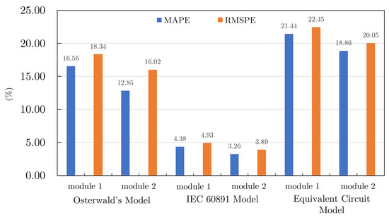
Figure 20.
Bar diagram of the MAPE and RMSPE of irradiance estimates using three CFMs for two PV modules of different service times.
Table 8 shows the results of the precision analysis per day, including the number of samples, the irradiance range, and the calculated metrics. Although on the first day, Figure 18a, irradiance levels of up to 1200 W/m2 are recorded, these values are excluded by the applied filter due to their short duration, as the pyranometer does not detect them, although the implemented system captures them. As a result, the range analyzed on this day is limited to approximately 820 W/m2. A similar behavior is observed on days 2 and 4, where the range is reduced to just over 400 W/m2. In contrast, day 3, Figure 18c, which is characterized by high intermittent cloudiness, includes data above 1000 W/m2. Thus, the results show a high similarity in accuracy metrics for days 1, 2, and 4 (low intermittency), with smaller errors in module 2 compared to module 1. On day 3 (high intermittency), the MAPE and RMSPE values were 6.36% and 6.86% for module 1, respectively, while for module 2, they were 5.25% and 5.96%. On day 4 for module 2, the measurements were oriented to overestimate the real values, with errors between 0.34 W/m2 and 10.75 W/m2 at low intermittency and between 18.20 W/m2 and 24.66 W/m2 at high intermittency. Thus, on day 4, module 2 shows an underestimation of 2.43 W/m2. Also, Table 8 shows systematic bias determined in W/m2. This same bias can be used to adjust the modules’ estimates. However, more dynamic models would be required that include an indicator of aging as the actual or current efficiency concerning the factory efficiency.
Table 8.
Irradiance estimation errors per day and PV modules for the best CFM.
Based on these results, we ranked the accuracy of the IEC model as a function of cloud intermittency. In addition, the average metrics for the low intermittency days (days 1, 2, and 4) were calculated and compared to those for the one high intermittency day (day 3). Therefore, we determined that the IEC model was most accurate in PV module 2 (no usage time), achieving 97.4% accuracy (2.6% error and 3.2% RMSPE) at low intermittency, while in PV module 1 (10 years of service), the accuracy was 96.29% (3.71% error and 4.28% RMSPE). These results are summarized in Table 9.
Table 9.
Accuracy errors of the IEC 60891 model considering low and high cloud intermittency and in-service time PV modules.
Based on all the results, we conclude that the developed system offers efficient and accurate performance in MPP tracking and temperature measurement in PV systems. The converter achieves 94% efficiency, while the improved MPPT IC algorithm achieves 99.88% efficiency, with fast convergence and lower MPP swing than the traditional IC algorithm. In addition, the temperature measurement system demonstrates reliability, with a variability of ±2 °C and a correlation coefficient of 0.9974 concerning reference values, validating its accuracy. On the other hand, the IEC model is the most accurate in the evaluation of CFMs, with errors of less than 5%, while the equivalent circuit model presents the highest uncertainty (>20%). The results also show the influence of aging on the performance of PV modules, with better estimates for the newly installed module.
4. Discussion
This section compares the results obtained from the CFM with other previous studies, evaluating their accuracy and applicability in different cloud conditions. Although the evaluated models agree with reference values, their practical application depends on certain idealized conditions. For example, uniform irradiance over the PV module surface and electrical behavior close to the maximum power point are assumed. These assumptions may not be met in real installations with dirt, partial shading, or localized thermal variations. Also, the model’s accuracy may decrease if the effects of PV module aging are not considered, so future implementations should explore incorporating dynamic correction factors. Furthermore, although the accuracy of the results is obtained directly by comparing the estimates with real values, it also depends on the accuracy of the implemented measurement systems, especially the maximum power tracking system with an improved IC algorithm, whose data are explicitly presented for replication. Therefore, the final results are compared with previous studies, considering the hardware and PV devices used, the conditions and irradiance ranges covered during data collection, and the estimation errors, as shown in Table 10. The main difference concerning previous work will be the errors in terms of MAE and RMS, which range between 1.08% and 5% and between 1.5% and 4.6%. The minimum and maximum errors in these terms with the proposed system achieved are between 2.6% and 6.36% of MAE and between 3.2% and 6.86% of RMS.
Table 10.
Comparison of estimation systems.
The system presented in [14] achieves the lowest MAE, with a value of 1.08%, using a small module of 10 W and an analytical model based on the equations of IEC 60891. However, the study covers a very limited irradiance range, between 880 and 920 W/m2. This irradiance range implies that, in a practical application, the accuracy of the model outside this range is uncertain, affecting the estimates’ reliability under different irradiance conditions. Also, the system presented in [16] records the lowest error, but in terms of RMS, with a value of 1.5%. This result was obtained using 12 mW monocrystalline cells and a model based on the characteristic equation of a diode with five parameters within an irradiance range of 300 to 600 W/m2. However, the analysis is limited. In addition, the study extends the evaluation range by considering an 87 W module with five years of use, covering irradiances from approximately 450 to 1000 W/m2, although with an increase in error of up to 3.2%. In [15], the authors use laboratory equipment to acquire the values of short-circuit current and peak current and apply them to a model of proportional relationship with irradiance. The estimation errors obtained vary between 3.6% (4.6%) and 3.9% (4.3%) between clear and cloudy days, respectively, using 245 W PV modules up to 5 years old in an irradiance range from 50 to 1000 W/m2. On the other hand, in [17], the authors also use the one-diode, five-parameter model with direct connection to a resistor under STC () conditions. In this case, the authors use PV emulators in an irradiance range from 200 to 1400 W/m2, obtaining errors lower than 5%.
The estimation system developed in this research is based on an Arduino Nano with an improved IC algorithm to eliminate oscillations at the point of maximum power. The system’s performance was evaluated in real conditions for four days, classifying irradiance changes into two categories according to cloud movement: slow and fast. Cloudy conditions prevailed, covering a wide range of irradiances above 1000 W/m2. As a sensing element, two 80 W monocrystalline PV modules were used, emulating their continuous operation as a generator.
Compared to [14], which also employs the IEC model and an MPPT algorithm, the proposed system offers a broader estimation capability, covering a wider range of irradiance and varying conditions. In contrast, the referenced approach is limited to 40 discrete irradiance levels. As for using other models, such as the one-diode, five-parameter model used in [16], although it has minimal errors, its range of analysis is limited. Similarly, in [17], the authors do not evaluate the system under real operating conditions. In both cases, their estimators only function as sensors when connected to a single fixed load (). In contrast, the proposed system offers dual operation, allowing estimation and power generation. In [15], the authors test the short-circuit model with average power modules, obtaining good results in terms of estimation over 16 months. These results are comparable to those obtained with the new module used in this study, with a 1% difference with respect to the old module, which is five years older than the one used in [15].
Although in terms of accuracy, the model used is comparable to that obtained with the new PV module, the degradation of the module with 10 years of service, as seen in Figure 18 affects the estimation. However, this effect can be corrected by adjusting the bias value to align it with the new PV module. Likewise, regarding the reproducibility of the estimation system, the proposed implementation takes advantage of the generated power, unlike previous studies, which makes it more suitable for environments where irradiance data are required without compromising PV power generation. Furthermore, its accuracy is comparable to that of previously described dedicated systems. In addition, independent of the data integration node, the system’s pyranometer, and the temperature measurement module, the maximum power point tracker (MPPT) operates with a 5 V power supply and a total power consumption of 32 mA. The MPPT system costs approximately 20 USD and has an estimated lifetime of 10 years under continuous and optimal operating conditions. Compared to commercial solutions based on irradiance sensors, such as the Davis Instruments model 6450 pyranometer valued at 225 USD, the developed proposal represents a cheaper alternative.
Finally, the research has certain limitations. On the one hand, the experiment was carried out on the rooftop of the building of the Professional School of Electronic Engineering of the National University San Antonio Abad del Cusco, where the photovoltaic modules and equipment are located. On the other hand, variable climatic conditions limited the continuity of the measurements, particularly in conditions of high irradiance. So, the experimental period was adjusted according to operational and climatic availability. Although the results show good accuracy in irradiance estimation, the tests were limited to four days in specific climatic conditions so that they cannot be represented in other geographical or seasonal environments. Furthermore, using a single type of PV module and NTC thermistors limits the system’s generalizability to other PV modules. Additionally, from a practical application point of view, the proposed system offers a high potential to be integrated into stand-alone PV systems (off-grid) and smart microgrids. Thanks to its low cost and low power consumption, it can function simultaneously as a power generator and irradiance sensor, allowing real-time monitoring of PV module performance without requiring expensive external sensors such as pyranometers. In microgrid environments, this type of system can operate as a distributed diagnostic node, facilitating load balancing, generation forecasting, and anomaly detection at the PV module level. These features make it a suitable solution for rural areas or isolated communities.
5. Conclusions and Future Works
This paper presents the design and development of a prototype for irradiance estimation based on evaluating three CFMs, integrating an MPPT system and temperature measurement using NTC thermistors. The selected CFMs use current and voltage in the MPP. The low-complexity MPPT system reduces the oscillations of the IC algorithm and provides key information for reproducibility. Of the three CFMs analyzed, the model based on the IEC 60891 equations showed the highest accuracy in irradiance estimation. This model showed an overall error of 3.89% when using a new PV module and 4.38% with a 10-year-old PV module. The MPPT system was implemented and analyzed on the rooftop of the Professional School of Electronic Engineering of the UNSAAC for 4 days. The irradiance patterns on these days could be classified into low and high cloudiness days, so the estimation results are divided into two. For low cloud conditions (130 to 820 W/m2), the error decreases to 2.6% with the new PV module and 3.71% with the old one; and for high cloud conditions (100 to 1110 W/m2), the error increases to 5.25% with the new PV module and 6.36% with the old one. Despite the increase in cloudy days, the system effectively detects rapid changes and shows an irradiance pattern very close to the readings of a reference instrument. Results indicate that integrating an MPPT controller with a current and voltage measurement system in PV modules with up to 10 years of operation allows the estimation of irradiance values and enables the analysis of their variability throughout the day. This dual functionality makes the system capable of operating simultaneously as a power generator and irradiance sensor.
Although the results obtained demonstrate a high accuracy of the proposed system under cloudy and variable irradiance conditions, it is acknowledged that the experimental period was limited to four days, mainly due to climatic and logistical constraints at the test site. Furthermore, the proportion of data collected under high irradiance conditions was low, which restricts the validation of the model under strong solar irradiance scenarios. Consequently, future work is proposed to extend the experimental cycle over different seasons, including extreme conditions and environments with high solar exposure, to evaluate the system’s long-term stability and seasonal adaptability. On the other hand, another future work of this study would be the extension of the methodology to PV arrays to evaluate its applicability in medium and large-scale solar generation systems. Also, the optimization of the MPPT algorithm to improve its performance in the face of rapid irradiance variations and its possible integration in remote monitoring platforms, such as SCADA or IoT platforms, using non-invasive current and voltage measurements at the output of the PV arrays. These estimates would allow the solution to be scaled up for application in microgrids or stand-alone PV systems of higher capacity. Also, future work could address the combination of IC algorithms with Perturbation and Observation (P&O) or Neural Networks to improve tracking under partial shading conditions for small and large PV systems, including an adaptive step size gradient based on dynamic adjustment of the rate of change of dP/dV to reduce convergence time using a higher frequency microcontroller such as the 72 MHz stm32f103c8t6. Finally, another avenue of future research is the performance of an interval analysis across different time windows to assess the variability of the estimated irradiance.
Author Contributions
Conceptualization and methodology, C.R.C.-N., A.P.L. and R.J.C.-C.; software, C.R.C.-N.; validation and formal analysis, C.R.C.-N. and R.J.C.-C.; investigation, C.R.C.-N. and R.J.C.-C.; resources, L.W.U.M., J.C.H.-L. and R.J.C.-C.; data curation, C.R.C.-N. and E.J.S.-C.; writing—original draft preparation, C.R.C.-N., E.M.-C. and E.J.S.-C.; writing—review and editing, all authors; visualization, L.W.U.M., A.P.L. and E.M.-C.; supervision, R.J.C.-C. and E.J.S.-C.; project administration, L.W.U.M. and R.J.C.-C.; funding acquisition, L.W.U.M., J.C.H.-L. and R.J.C.-C. All authors have read and agreed to the published version of the manuscript.
Funding
This work was funded by the Universidad Nacional San Antonio Abad del Cusco (UNSAAC) through the projects of the Professional School of Electronic Engineering and partially by the Universidad Politécnica Salesiana under the Fog Computing Simulation project.
Data Availability Statement
Data are contained within the article.
Acknowledgments
We thank the Institutional Laboratory for Research, Entrepreneurship and Innovation in Automatic Control Systems, Automation and Robotics (LIECAR) and the Laboratory of Renewable Energy, Optical Communications Engineering and Environmental Technology (TESLA), both from the Universidad Nacional de San Antonio Abad del Cusco (UNSAAC).
Conflicts of Interest
The authors declare no potential conflicts of interest.
References
- Hossain, M.S.; Wadi Al-Fatlawi, A.; Kumar, L.; Fang, Y.R.; Assad, M.E.H. Solar PV high-penetration scenario: An overview of the global PV power status and future growth. Energy Syst. 2024, 1–57. [Google Scholar] [CrossRef]
- Swadi, M.; Kadhim, D.J.; Salem, M.; Tuaimah, F.M.; Majeed, A.S.; Alrubaie, A.J. Investigating and predicting the role of photovoltaic, wind, and hydrogen energies in sustainable global energy evolution. Glob. Energy Interconnect. 2024, 7, 429–445. [Google Scholar] [CrossRef]
- Feldman, D.; Zuboy, J.; Dummit, K.; Stright, D.; Heine, M.; Mirletz, H.; Margolis, R. Winter 2024 Solar Industry Update; Technical Report; National Renewable Energy Laboratory (NREL): Golden, CO, USA, 2024. [Google Scholar]
- Balakrishnan, P. Global Renewable Energy Transition Challenges and Strategic Solutions. In Geopolitical Landscapes of Renewable Energy and Urban Growth; IGI Global Scientific Publishing: Hershey, PA, USA, 2025; pp. 63–96. [Google Scholar]
- He, L.; Liu, Y.L.; Tang, Z.J.; Sun, T.; Yan, Y.M.; Xia, Y.F.; Feng, H.S.; Ye, W. Intensified excessive wastage of key raw metals with expansion of global wind and solar photovoltaic energy development. Resour. Conserv. Recycl. 2025, 215, 108127. [Google Scholar] [CrossRef]
- Frolova, M.; Osorio-Aravena, J.C.; Pérez-Pérez, B.; Pasqualetti, M.J. Abandoning renewable energy projects in Europe and South America: An emerging consideration in the recycling of energy landscapes. Energy Sustain. Dev. 2025, 85, 101676. [Google Scholar] [CrossRef]
- Galvez, D.P.C.; Revinova, S.Y. Energy transition as a path to sustainable development in Latin American countries. Unconv. Resour. 2025, 6, 100157. [Google Scholar]
- Ministerio de Energía y Minas del Perú. Programa Masivo Fotovoltaico. 2020. Available online: https://www.gob.pe/institucion/minem/noticias (accessed on 27 February 2025).
- Centro Nacional de Planeamiento Estratégico (CEPLAN). Cobertura del Servicio de Energía Eléctrica a Nivel Nacional. 2023. Available online: https://observatorio.ceplan.gob.pe/ficha/t39 (accessed on 27 February 2025).
- Terrones Rabanal, M. Diseño De Un Sistema De Telemetría Utilizando Tecnología Gsm, Para Monitorear Variables Fotovoltaicas Domesticas Rurales; Universidad Nacional Tecnológica de Lima Sur: Lima, Perú, 2017; Available online: https://repositorio.untels.edu.pe/jspui/handle/20.500.14717/410 (accessed on 27 February 2025).
- Cotfas, D.T.; Cotfas, P.A.; Machidon, O.M. Study of temperature coefficients for parameters of photovoltaic cells. Int. J. Photoenergy 2018, 2018, 5945602. [Google Scholar] [CrossRef]
- Chikh, A.; Chandra, A. An optimal maximum power point tracking algorithm for PV systems with climatic parameters estimation. IEEE Trans. Sustain. Energy 2015, 6, 644–652. [Google Scholar] [CrossRef]
- Carvalho, I.F.; Correa, M.B. Techniques of solar irradiance estimation from datasheet information of photovoltaic panels. In Proceedings of the 2019 IEEE 15th Brazilian Power Electronics Conference and 5th IEEE Southern Power Electronics Conference (COBEP/SPEC), Santos, Brazil, 1–4 December 2019; pp. 1–6. [Google Scholar]
- Moshksar, E.; Ghanbari, T. Real-time estimation of solar irradiance and module temperature from maximum power point condition. IET Sci. Meas. Technol. 2018, 12, 807–815. [Google Scholar] [CrossRef]
- Abe, C.F.; Dias, J.B.; Notton, G.; Faggianelli, G.A. Experimental application of methods to compute solar irradiance and cell temperature of photovoltaic modules. Sensors 2020, 20, 2490. [Google Scholar] [CrossRef]
- Carrasco, M.; Laudani, A.; Lozito, G.M.; Mancilla-David, F.; Riganti Fulginei, F.; Salvini, A. Low-cost solar irradiance sensing for pv systems. Energies 2017, 10, 998. [Google Scholar] [CrossRef]
- Laudani, A.; Lozito, G.M.; Riganti Fulginei, F. Irradiance sensing through PV devices: A sensitivity analysis. Sensors 2021, 21, 4264. [Google Scholar] [CrossRef] [PubMed]
- IEC 60891; Photovoltaic Devices. Procedures for Temperature and Irradiance Corrections to Measured IV Characteristics. International Electrotechnical Commission: Geneva, Switzerland, 2009.
- Fuentes, M.; Nofuentes, G.; Aguilera, J.; Talavera, D.; Castro, M. Application and validation of algebraic methods to predict the behaviour of crystalline silicon PV modules in Mediterranean climates. Sol. Energy 2007, 81, 1396–1408. [Google Scholar] [CrossRef]
- Hassan, S.Z.; Li, H.; Kamal, T.; Ahmad, J.; Riaz, M.H.; Khan, M.A. Performance of different MPPT control techniques for photovoltaic systems. In Proceedings of the 2018 International Conference on Electrical Engineering (ICEE), Istanbul, Turkey, 3–5 May 2018; pp. 1–6. [Google Scholar]
- Malkawi, A.M.; Alsaqqa, Z.A.; Al-Mosa, T.O.; Wa’el M, J.A.; Sadeddin, M.M.; Al-Quraan, A.; Al Mashagbeh, M. Maximum Power Point Tracking Enhancement for PV in Microgrids Systems Using Dual Artificial Neural Networks to Estimate Solar Irradiance and Temperature. Results Eng. 2025, 25, 104275. [Google Scholar] [CrossRef]
- Srivastava, V.; Sharma, U.; Schaub, J.; Pischinger, S. Adaptive control concepts using radial basis functions and a Kalman filter for embedded control applications. Int. J. Engine Res. 2024, 25, 125–139. [Google Scholar] [CrossRef]
- Yi, V.Q.J.; Han, P.Y.; You, L.Z.; Yin, O.S.; Khoh, W.H. Predicting churn with filter-based techniques and deep learning. Int. J. Electr. Comput. Eng. 2024, 14, 2135–2144. [Google Scholar]
- Abe, C.F.; Dias, J.B.; Notton, G.; Poggi, P. Computing Solar Irradiance and Average Temperature of Photovoltaic Modules from the Maximum Power Point Coordinates. IEEE J. Photovolt. 2020, 10, 655–663. [Google Scholar] [CrossRef]
- Mahmoud, Y. A Model-based MPPT with Improved Tracking Accuracy. In Proceedings of the IECON 2018—44th Annual Conference of the IEEE Industrial Electronics Society, Washington, DC, USA, 21–23 October 2018; pp. 1609–1612. [Google Scholar] [CrossRef]
- Scolari, E.; Sossan, F.; Paolone, M. Photovoltaic-Model-Based Solar Irradiance Estimators: Performance Comparison and Application to Maximum Power Forecasting. IEEE Trans. Sustain. Energy 2018, 9, 35–44. [Google Scholar] [CrossRef]
- Hooshmand, M.; Yaghobi, H.; Jazaeri, M. Irradiation and Temperature Estimation with a New Extended Kalman Particle Filter for Maximum Power Point Tracking in Photovoltaic Systems. Int. J. Eng. 2023, 36, 1099–1113. [Google Scholar] [CrossRef]
- Malkawi, A.M.A.; Odat, A.; Bashaireh, A. A Novel PV Maximum Power Point Tracking Based on Solar Irradiance and Circuit Parameters Estimation. Sustainability 2022, 14, 7699. [Google Scholar] [CrossRef]
- Prasetyono, E.; Sunarno, E.; Imam, M.S. Real-Time Irradiance Estimation Based on Maximum Power Current of Photovoltaic. In Proceedings of the 2019 4th International Conference on Information Technology, Information Systems and Electrical Engineering (ICITISEE), Yogyakarta, Indonesia, 20–21 November 2019; pp. 507–510. [Google Scholar] [CrossRef]
- Coelho, R.F.; Concer, F.M.; Martins, D.C. A MPPT approach based on temperature measurements applied in PV systems. In Proceedings of the 2010 IEEE International Conference on Sustainable Energy Technologies (ICSET), Kandy, Sri Lanka, 6–9 December 2010; pp. 1–6. [Google Scholar] [CrossRef]
- Hyndman, R.J.; Koehler, A.B. Another look at measures of forecast accuracy. Int. J. Forecast. 2006, 22, 679–688. [Google Scholar] [CrossRef]
- Wong, W.K.; Bai, E.; Chu, A.W.C. Adaptive time-variant models for fuzzy-time-series forecasting. IEEE Trans. Syst. Man Cybern. Part B Cybern. 2010, 40, 1531–1542. [Google Scholar] [CrossRef] [PubMed]
- Mohan, N.; Robbins, W.; Undeland, T. Electrónica de Potencia; Mc Graw Hill: New York, NY, USA, 2009. [Google Scholar]
- Texas Instruments. Basic Calculation of a Buck Converter’s Power Stage; Application Report-SLVA477B, Rev. B.; Texas Instruments: Dallas, TX, USA, 2015; Available online: https://www.ti.com/lit/pdf/slva477 (accessed on 27 February 2025).
- Texas Instruments. Bootstrap Circuitry Selection for Half-Bridge Configurations; Application Report SLUA887; Texas Instruments: Dallas, TX, USA, 2018; Available online: https://www.ti.com/lit/pdf/slua887 (accessed on 12 March 2025).
- Chellakhi, A.; Beid, S.E.; Abouelmahjoub, Y.; Doubabi, H. An Enhanced Incremental Conductance MPPT Approach for PV Power Optimization: A Simulation and Experimental Study. Arab. J. Sci. Eng. 2024, 49, 16045–16064. [Google Scholar] [CrossRef]
- Shiau, J.K.; Wei, Y.C.; Chen, B.C. A study on the fuzzy-logic-based solar power MPPT algorithms using different fuzzy input variables. Algorithms 2015, 8, 100–127. [Google Scholar] [CrossRef]
- Cotfas, D.T.; Ursutiu, D.; Samoila, C. The Methods to Determine the Series Resistance and the Ideality Factor of Diode for Solar Cells-Review. In Proceedings of the 2012 13th International Conference on Optimization of Electrical and Electronic Equipment, Brasov, Romania, 24–26 May 2012; pp. 966–972. [Google Scholar]
- SolarWorld. SW 80 Mono RHA Photovoltaic Module Data Sheet; SolarWorld AG: Bonn, Germany, 2016; Available online: https://www.enfsolar.com/Product/pdf/Crystalline/57733b05c7f91.pdf (accessed on 10 March 2025).
- Nishioka, K.; Miyamura, K.; Ota, Y.; Akitomi, M.; Chiba, Y.; Masuda, A. Accurate measurement and estimation of solar cell temperature in photovoltaic module operating in real environmental conditions. Jpn. J. Appl. Phys. 2018, 57, 08RG08. [Google Scholar] [CrossRef]


Disclaimer/Publisher’s Note: The statements, opinions and data contained in all publications are solely those of the individual author(s) and contributor(s) and not of MDPI and/or the editor(s). MDPI and/or the editor(s) disclaim responsibility for any injury to people or property resulting from any ideas, methods, instructions or products referred to in the content. |
© 2025 by the authors. Licensee MDPI, Basel, Switzerland. This article is an open access article distributed under the terms and conditions of the Creative Commons Attribution (CC BY) license (https://creativecommons.org/licenses/by/4.0/).