Abstract
Aiming at the problems of existing time series data clustering methods, such as the lack of similarity metric universality, the influence of dimensional catastrophe, and the limitation of feature expression ability, a time series data clustering method based on unsupervised contrasting learning (UCL-TSC) is proposed. The method first utilizes Residual, TCN, and CNN-TCN to construct multi-view representations of spatial, temporal, and spatial–temporal features of time series data, and adaptively fuses complementary information to enhance feature extraction capabilities. Subsequently, positive and negative sample pairs are constructed based on nearest neighbor and pseudo-clustering label information. Finally, a contrast loss function consisting of feature loss, clustering loss, and a regularization term is designed to facilitate the model in achieving compact intra-cluster and sparse inter-cluster clustering effects in the clustering process. The experimental results on the UCR dataset show that UCL-TSC performs well with respect to several evaluation indexes, such as clustering accuracy, normalized information degree, and purity, and is more effective in learning time series data features and achieving accurate clustering compared to traditional clustering and deep clustering methods.
1. Introduction
As one of the basic tasks in the field of data mining, clustering can classify data into different clusters based on the similarity of features and attributes of the data points, so that the points in the same cluster are more similar to each other compared to the points in other clusters. Clustering algorithms have a wide range of applications in the fields of image denoising, data dimensionality reduction, medical diagnosis, etc. A variety of clustering strategies have been developed in the face of different types of datasets. With respect to time series data clustering (TSC), existing clustering methods can be broadly categorized into six types: partitional clustering (k-means [1,2,3], k-medoids [4,5,6]), hierarchical clustering (AGNES [7], DIANA [8]), density-based clustering (DBSCAN [9,10], OPTICS [11,12], HDBSCAN [13,14,15]), graph-based clustering (spectral clustering [16,17,18], graph partitioning [19]), model-based clustering [20,21,22], and deep-learning-based clustering (contrastive learning methods [23,24,25,26,27,28], non-contrastive learning methods [29,30,31,32,33]).
Despite their widespread use in TSC tasks, traditional clustering methods, such as partitional clustering, hierarchical clustering, and density-based clustering, often struggle to handle high-dimensional time series data due to their sensitivity to noise and parameter selection. In contrast, by leveraging neural networks to capture temporal dependencies and complex patterns, deep clustering has demonstrated superior performance in clustering tasks. As a type of deep clustering method, the core idea of contrastive learning is to learn feature representations of data by maximizing the similarity between positive sample pairs and minimizing the similarity between negative sample pairs. This ultimately ensures that positive pairs are pulled closer in the embedding space while negative pairs are pushed apart. While contrastive learning has achieved remarkable success in the image domain, its direct application to TSC tasks still faces the following challenges.
First, sensitivity to the construction of positive and negative sample pairs. Traditional contrastive learning methods typically rely on data augmentation to generate positive samples. However, the dynamics and complexity of time series make it difficult for sample pairs to capture true similarities based on simple augmentation.
Second, insufficient utilization of multi-view features. Existing contrastive learning frameworks mainly focus on single-view feature representations, making it challenging to capture complementary spatial–temporal features.
Third, the disconnection between feature representation and clustering objectives. Current methods often employ generic contrastive loss functions, such as information noise contrastive estimation (InfoNCE), which are difficult to optimize specifically for clustering objectives, leading to inconsistency between the feature space and clustering structure.
To address the above problems, this paper proposes an unsupervised contrastive-learning-based clustering method (UCL-TSC) for time series data. The clustering performance is effectively improved by multi-view feature fusion, pseudo-label-guided sample pair construction, and contrastive loss function. The main contributions of this paper are as follows.
(1) Multi-view feature fusion. A multi-view representation of spatial, temporal, and spatial–temporal features of time series data is constructed using Residual, TCN, and CNN-TCN models, and complementary information is fused through adaptive weight learning to enhance the feature extraction capability of time series data.
(2) Construction of positive and negative sample pairs. The approach proposed in this study fully considers the nearest neighbor and pseudo-clustering label information to construct positive and negative sample pairs, i.e., two samples are treated as positive sample pairs if they are nearest neighbors and assigned to the same class, and as negative sample pairs otherwise.
(3) Design of the contrastive loss function. The contrastive loss function is mainly composed of three parts: feature-level loss, clustering loss, and a regularization term, which together promote compact intra-cluster and sparse inter-cluster clustering effects during the clustering process.
(4) Design of experiments. To verify the clustering performance of the model, we conduct analytical experiments and comparative experiments on several UCR datasets to validate the effectiveness of the model.
The remaining sections of this paper are specifically structured as follows. Section 2 provides a description of the TSC task. Section 3 details our proposed clustering method based on unsupervised contrastive learning (UCL-TSC). Section 4 describes the dataset used to validate the model, the evaluation metrics, the experiments conducted, and the specific conclusions. Section 5 summarizes the article.
2. Task Setting
TSC aims to classify series with similar dynamic patterns, trend characteristics, or structural properties into the same category based on the intrinsic similarities between time series data, while series from different categories are significantly distinct. The core task of TSC is the process of mining data for dependencies and pattern differences, mapping them to corresponding clusters. Analyzed mathematically, this process can be expressed in the form of the following equation.
where C denotes the grouping information of the time series data, denotes a set of time series, and each time series Xi consists of a vector of length m. The value of C obtained after clustering needs to satisfy the following conditions.
3. The Proposed Method
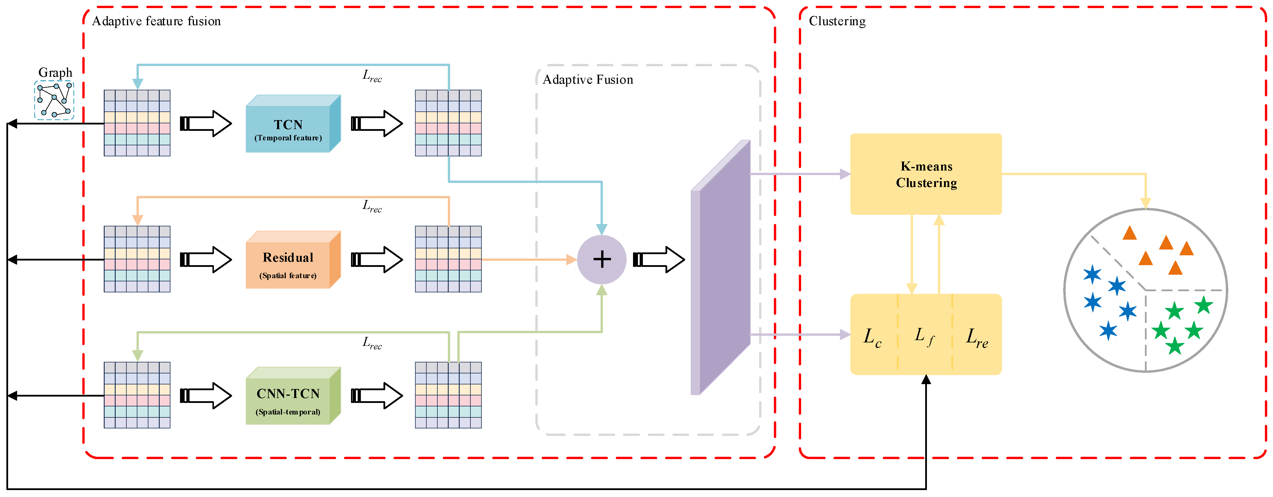
Our proposed clustering model for time series data based on unsupervised comparative learning is shown in Figure 1. The model consists of three main modules: multi-view feature fusion, positive and negative sample pair construction, and clustering. In the remainder of this section, we provide a detailed description of these three modules, the overall target loss, and the training strategy.
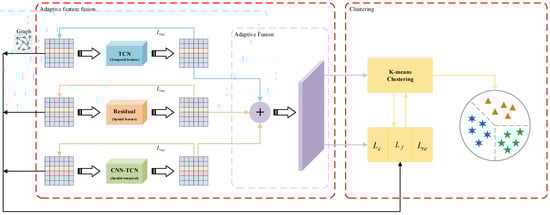
Figure 1.
The UCL-TSC framework. The Residual module extracts spatial features via 1D CNN with residual concatenation; the TCN module captures temporal dependencies using dilated causal convolution; the CNN-TCN module fuses spatial features with temporal features; and the adaptive fusion layer integrates multi-view features using learnable weights.
3.1. Multi-View Feature Fusion
In this paper, we consider extracting the temporal, spatial, and spatial–temporal features of the data separately, based on which we learn a consensus representation shared by the three features in order to obtain a unique clustering result. Specifically, let , , and denote the network models for extracting temporal features, spatial features, and spatial–temporal features, respectively, and let , , and be the parameters of the corresponding network models.
For temporal feature extraction, a temporal convolutional neural network (TCN) is used in this paper for the smoothing and compression of time series data. TCN is a network model that can handle time series data with the core of dilated causal convolution, proposed by Shaojie Bai et al. in 2018. The exponential multiplicative expansion of the dilated causal convolution’s sense field enables it to cover all valid inputs of the time series, leading to better fusion of information and effective modeling of long-term patterns in the series. Given the input , the temporal features extracted by the TCN are represented as in Equation (4).
For spatial feature extraction, a 1D convolutional neural network (CNN) is used to smooth and compress the time series data, introducing residual connections to strengthen the spatial feature extraction capability of the model. Given the input , the spatial features extracted by the Residual module are represented as in Equation (5).
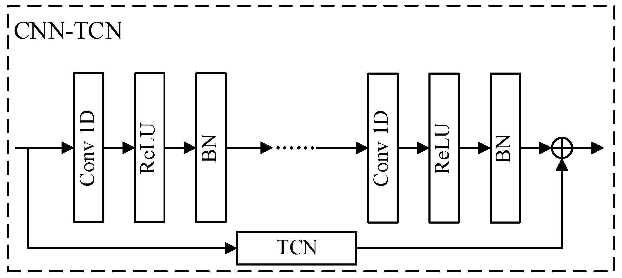
For spatial–temporal feature extraction, this paper adopts the structure of TCN and CNN fusion for the smoothing and compression of time series data, as shown in Figure 2. Given the input , the spatial–temporal features extracted by TCN-CNN are represented as in Equation (6).
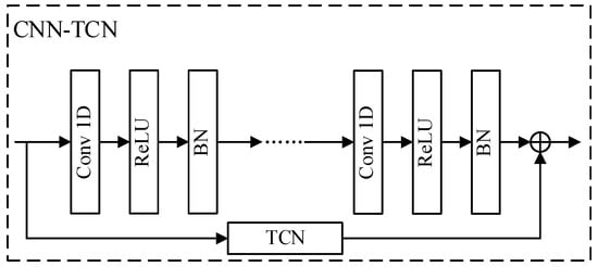
Figure 2.
Structure of the CNN-TCN model.
To enable each network model to capture valuable deep features, this paper introduces a reconstructed loss with reference to the autoencoder, as shown in Equation (7).
After obtaining separate feature representations, an adaptive fusion mechanism is introduced to fuse the three features to obtain a consensus, and the fused feature representation is shown in Equation (8).
where denotes the weight of the feature representation, which is adaptively determined by the trainable parameter of each network model. The specific formula is . The weights are updated based on the feature distribution of the training data, such a distribution enabling the model to automatically adjust the importance of each view feature according to different input data. This adaptive mechanism helps to avoid drastic changes in feature representation, thus stabilizing the model’s learning process.
3.2. Positive and Negative Sample Pair Construction
In contrastive learning, the construction of positive and negative sample pairs plays a crucial role. In the task of TSC, traditional comparative learning methods usually treat the original data and the augmented data as a pair of positive samples, while all other data are treated as negative samples. This violates the principle of intra-class compactness. Literature [34] considers the construction of positive and negative sample pairs by combining nearest-neighbor and pseudo-clustering label information, and the effectiveness of the method is confirmed by simulation experiments. In this paper, we cite the positive–negative sample pair construction method in the literature and first construct the nearest neighbor graph G of each sample as follows.
where denotes the set of instances closest to .
The consensus representation obtained after adaptive feature fusion is subjected to k-means clustering to produce an indication matrix . In this matrix, = 1 if and only if the ith and jth samples are assigned to the same category. The constructed set of positive sample pairs, Pi, and the set of negative sample pairs. Ni, are as follows.
3.3. Contrastive Loss Function
3.3.1. Clustering Loss
For a given time series dataset, assuming the number of clusters is K, we design the following clustering loss function inspired by the literature [35].
where denotes the consensus feature representation of the kth cluster obtained after running three network models. denotes the features of the kth cluster obtained after running a single network model, denotes the spatial feature representation of the kth cluster, denotes the temporal feature representation of the kth cluster, and denotes the spatial–temporal feature representation of the kth cluster. denotes the temperature parameter. is the similarity function, which is measured here using the cosine similarity, i.e., .
3.3.2. Feature-Level Loss
Section 3.2 constructs corresponding pairs of positive and negative samples for the given time series data, for which we design the following feature-level loss to better distinguish between similar and dissimilar instances. The feature-level loss consists of a positive sample pair loss and a negative sample pair loss.
where denotes the temperature parameter, denotes the consensus feature representation of the ith sample after running three network models, denotes the feature of the ith sample after running a single network model, denotes the spatial feature representation of the ith sample, denotes the temporal feature representation of the ith sample, and denotes the spatial–temporal feature representation of the ith sample.
In Equation (13), all pairs of negative samples have the same weight. This can cause the model to ignore the treatment of difficult negative and false-negative samples during training, leading to the possibility of overdispersion of similar samples and under-separation of dissimilar samples. To achieve intra-cluster compactness and inter-cluster sparsity, this paper dynamically adjusts the weights of negative sample pairs according to the cluster center similarity, i.e., the weights of negative samples within the same cluster are reduced, and the weights of negative samples between different clusters are increased. The adjusted feature-level loss is as follows.
where denotes the clustering center of the cluster to which the ith sample belongs.
3.3.3. Regularization Term
To prevent the clustering center from degrading and to improve the clustering performance, we introduce a regularization term. Through this regularization term, the model can learn a more discriminative and uniformly distributed feature representation, which is calculated as follows.
Combining the three loss functions, the contrastive loss values during training are as follows.
where and are the weights of clustering loss and feature-level loss, respectively. From the theoretical point of view, the reconstructed loss, Lrec, is a convex function of the mean square error, which can be stabilized and converged by the gradient descent method during the optimization process. The design of the clustering loss, Lc, and the feature-level loss, Lf, draws on the framework of contrastive learning, forming a clear optimization direction by maximizing the similarity of the positive sample pairs and minimizing the similarity of the negative sample pairs. The regularization term, Lr, avoids clustering center degradation by constraining the uniformity of feature distribution.
3.4. Training Process
In the initial phase of training, the TCN, Residual, and CNN-TCN modules are first trained to obtain better , , and parameters, and the loss function is the reconstructed loss in Equation (7). Finally, the k-means algorithm is executed on the consensus representation to obtain the final clustering results. The training process of the model is shown in Algorithm 1.
| Algorithm 1 Training Algorithm |
| Input: Time series data X, number of cluster K, batch size B. Output: The clustering results.
|
4. Experimental Evaluation
4.1. Experimental Dataset and Evaluation Indicators
To evaluate the performance of UCL-TSC, we conducted experiments on the publicly available UCR dataset (https://www.cs.ucr.edu/~eamonn/time_series_data_2018/, accessed on 15 February 2025). Each dataset consists of two parts, the training set and the test set. We fused the two datasets and used the entire data in our experiments. The UCR datasets come from multiple subject areas. Twelve datasets are selected here to cover diverse domains, varying sequence lengths, and complex category structures, as shown in Table 1, to verify the model’s generalization ability. The selection criteria are as follows.

Table 1.
Introduction to the selected UCR datasets.
First, the diversity of domains is considered. The datasets cover different sources such as ECG, EOG, image, sensor, and motion to avoid domain bias.
Second, the range of sequence lengths is considered. Sequence lengths span from 80 to 1250 to test the model’s ability to model long- and short-term dependencies.
Third, the difference in the number of categories is considered. The number of categories ranges from two to 12 to evaluate the model’s clustering stability under different category complexities.
Fourth, sample size is considered. Different sample sizes are used to validate the model’s adaptability to data sparsity.
To better quantify the model performance and compare it with that of other methods, unsupervised clustering accuracy (ACC), normalized mutual information (NMI), purity (PUR), F-score, Rand Index, reconstructed loss, and contrastive loss are selected as evaluation indicators in this paper. For these metrics, higher values indicate better model performance.
4.2. Experimental Details
We compared the UCL-TSC algorithm with traditional clustering and deep clustering methods. We ran k-means, Randomnet [32], KSC [36], k-shape [37], SPF [38], SPIRAL [39], kDBA [40], IDEC [41], DTC [42], and MiniRocket [43] on the same UCR dataset. Among the above methods, k-means, KSC, k-shape, and kDBA are clustering techniques based on raw data, while Randomnet, IDEC, DTC, and MiniRocket are deep learning clustering methods.
The experiments conducted in this paper are in the Python language, version 3.8, accelerated by NVIDIA GeForce RTX2080 GPU and CUDA 12.2, using a pytorch deep learning framework. The parameter settings for the UCL-TSC algorithm are shown in Table 2.
Table 2.
Parameter settings for the UCL-TSC algorithm.
4.3. Experimental Results
4.3.1. Analysis of UCL-TSC Performance
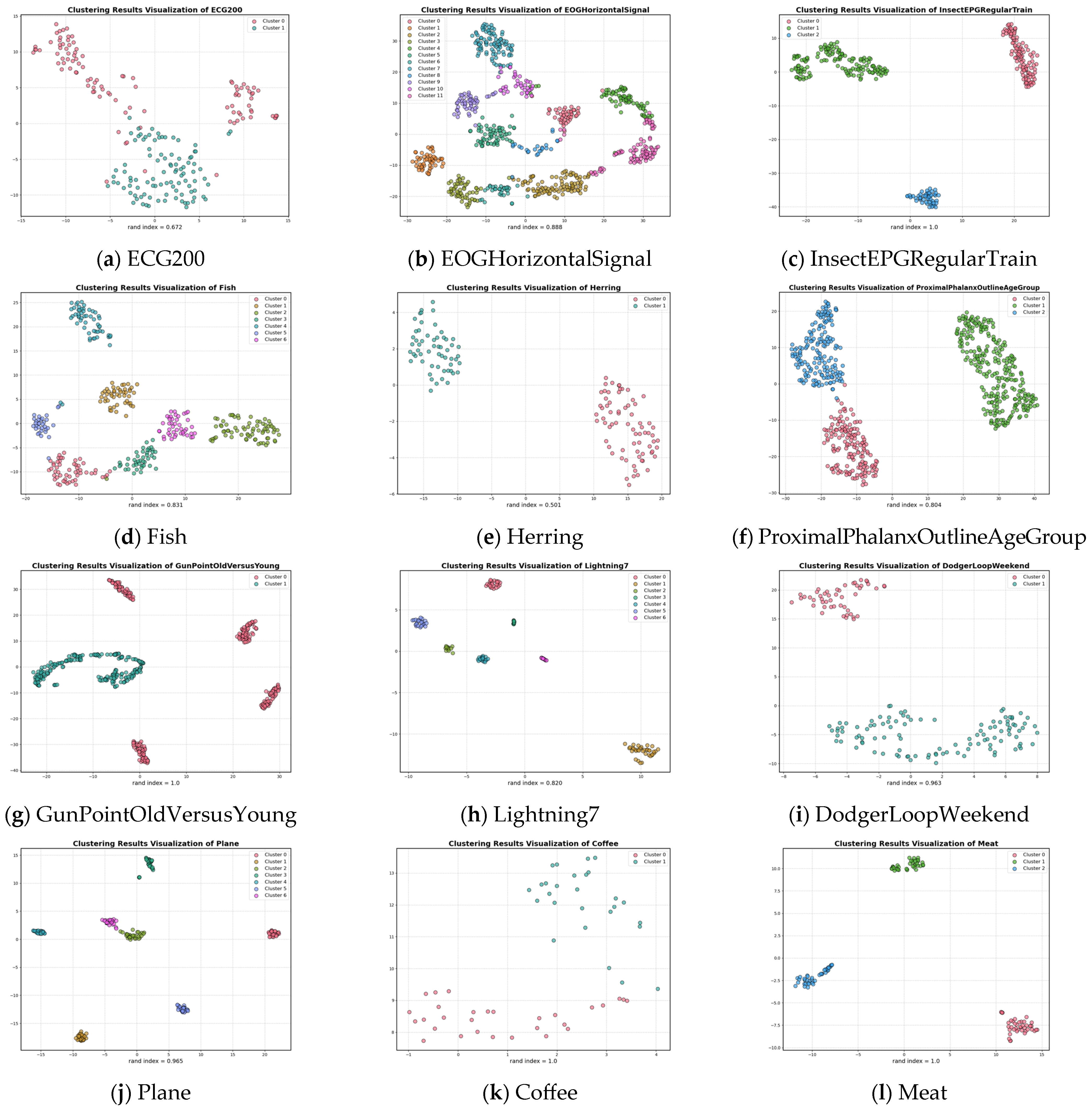
To visualize the performance of UCL-TSC, this section focuses on the twelve datasets listed in this paper. The corresponding ACC, NMI, PUR, F-score, and Rand Index values are provided, the graph of contrastive loss with respect to the epoch is plotted, and the clustering results are visualized using the T-SNE algorithm. The evaluation metrics of UCL-TSC with respect to the twelve example datasets are shown in Table 3.
Table 3.
Comparison of evaluation metrics for the twelve example datasets.
From Table 3, it can be seen that the UCL-TSC algorithm achieves better clustering results for data with different time series lengths, different sample sizes, and different numbers of clusters. In particular, all the indexes for the InsectEPGRegularTrain, Coffee, and Meat datasets can reach 1.000.
A visual illustration of the clustering results for the 12 datasets is provided in Figure 3. When the number of clusters is two, three, four and seven, the UCL-TSC algorithm is able to cluster the corresponding time series samples and identify the correct clusters. When the number of clusters is 12, although the UCL-TSC algorithm is able to identify the correct clusters, there is a situation where individual samples are far from the center of the corresponding cluster. In this paper, we analyze the datasets with a Rand Index value lower than 0.9 after clustering and find that these datasets generally have high intra-class variability and relatively low cluster separability, resulting in the phenomenon of overlapping clusters and, therefore, relatively low classification results. Combined with Figure 3, although the Rand indexes of these datasets are lower than 0.9 after clustering, UCL-TSC is able to better identify the clustering centers of the clusters and classify the corresponding data into the clusters to which they belong.
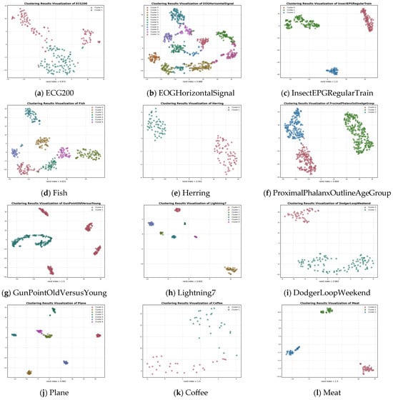
Figure 3.
Cluster visualization plots for different datasets.
4.3.2. Analysis of Contrastive Loss
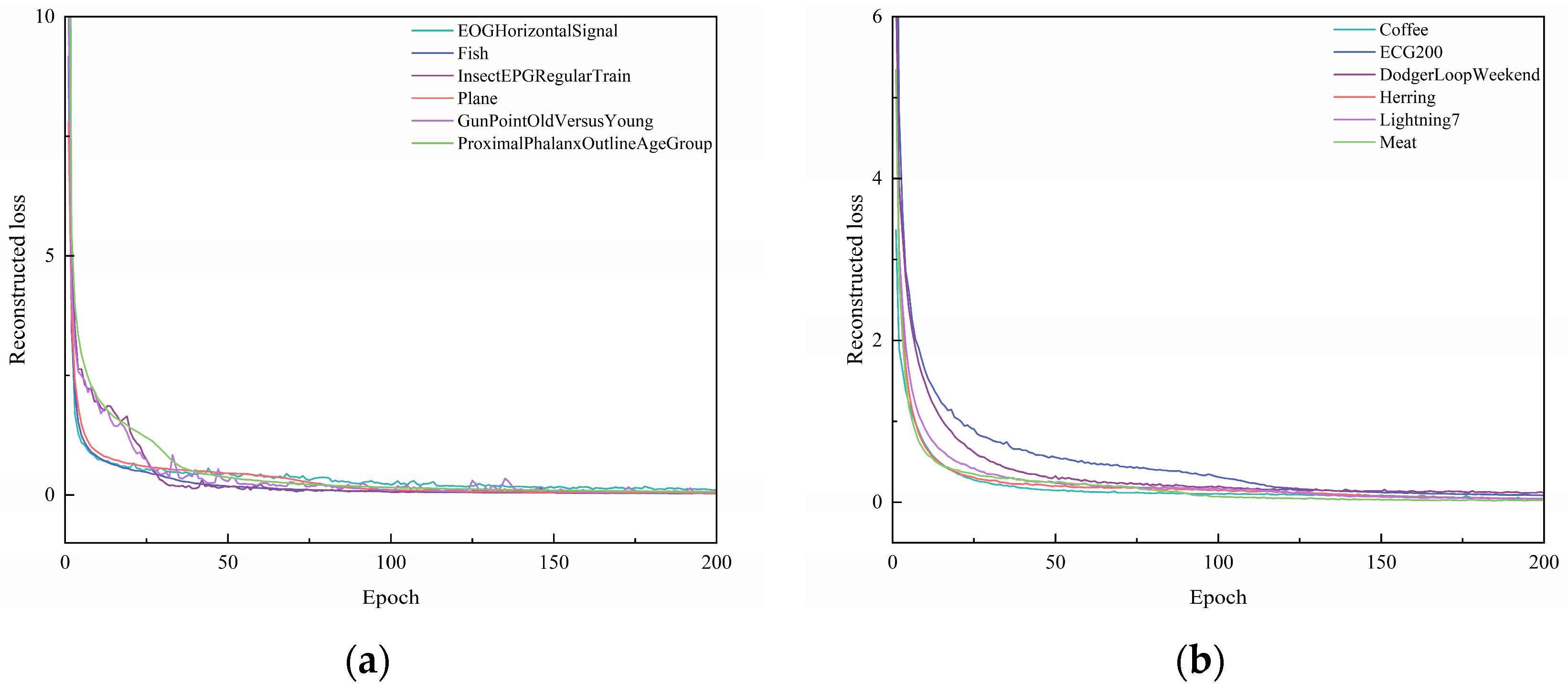
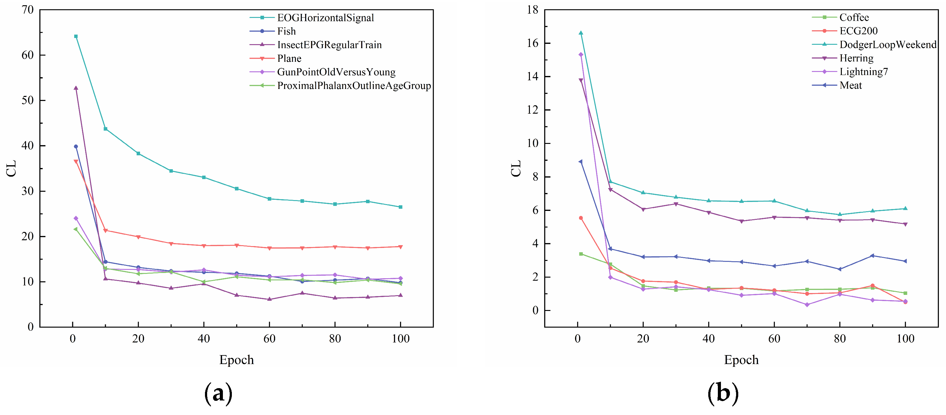
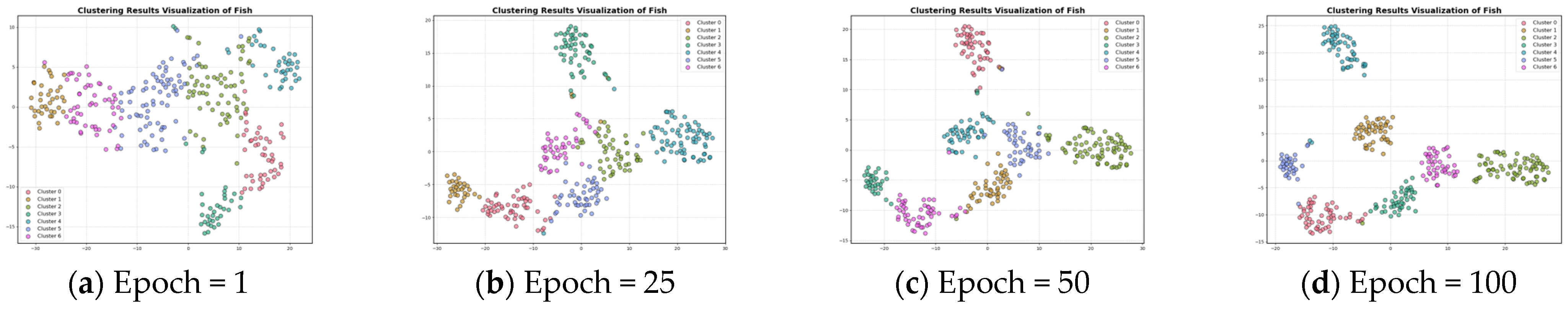
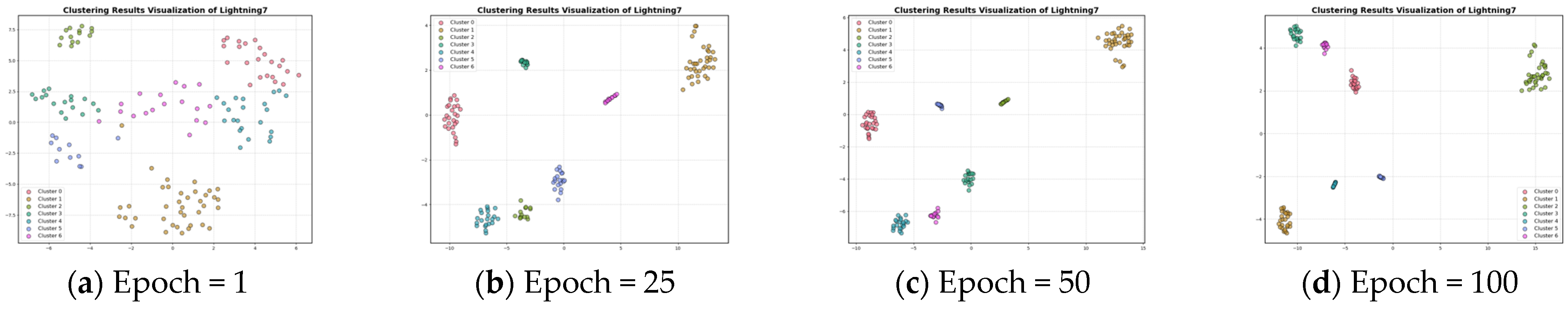
In Section 3.3, the contrastive loss function is proposed. To visualize the role of the contrast loss function for clustering, the curves of reconstruction loss and contrastive loss with respect to epochs are given in Figure 4 and Figure 5. Figure 6 and Figure 7 show the results of feature visualization corresponding to the 1st, 25th, 50th, and 100th epoch of the Fish and Lightning7 datasets during the training process.

Figure 4.
Plot of reconstructed loss as epochs change. (a) Reconstructed loss of EOGHorizontalSignal, Fish, InsectEPGRegularTrain, Plane, GunPointOldVersusYoung, ProximalPhalanxOutlineAgeGroup. (b) Reconstructed loss of Coffee, ECG200, DodgerLoopWeekend, Herring, Lightning7, Meat.
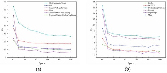
Figure 5.
Plot of contrastive loss as epochs change. (a) Contrastive loss of EOGHorizontalSignal, Fish, InsectEPGRegularTrain, Plane, GunPointOldVersusYoung, ProximalPhalanxOutlineAgeGroup. (b) Contrastive loss of Coffee, ECG200, DodgerLoopWeekend, Herring, Lightning7, Meat.
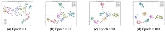
Figure 6.
Feature visualization of the Fish dataset during clustering.
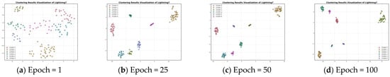
Figure 7.
Feature visualization of the Lightning7 dataset during clustering.
From Figure 4, it can be seen that, with the increase in epochs, the reconstruction loss during the training process of different datasets gradually decreases. When the epoch = 50, the change in the reconstruction loss of several datasets tends to stabilize. When the epoch = 125, the reconstruction loss during the training process of all ten datasets tends to stabilize. This shows that the UCL-TSC algorithm proposed in the paper can better extract the features of time series data, laying a good foundation for subsequent clustering. As can be seen in Table 4, the standard deviation of the loss values for multiple experiments for each dataset is below 1 × 10⁻⁶, indicating that the model convergence is stable.
Table 4.
Means and standard deviations of contrastive loss values from multiple experiments.
Figure 5 presents the plot of contrastive loss as epochs change during the training process for the ten datasets. It can be seen that the change in contrast loss tends to stabilize with the increase in epochs. Combined with Figure 6 and Figure 7, it can be observed that, with the increase in epochs, the distance between different clusters gradually increases, and the distribution of the samples within the same cluster becomes more and more compact. This indicates that the contrast loss function proposed in the paper plays an important role in the clustering of time series data.
4.3.3. Comparison Experiment
In this section, we compare the performance of the UCL-TSC algorithm proposed in this paper with that of ten other clustering algorithms, namely k-means, KSC, k-shape, SPF, SPIRAL, kDBA, IDEC, DTC, MiniRocket, and Randomnet, using the same dataset for the Rand Index. A larger Rand Index indicates better clustering performance. The partial results obtained are shown in Table 5, with the optimal and sub-optimal results highlighted in bold and underlined, respectively.
Table 5.
Comparison of the Rand Index with (a) k-means, k-shape, KSC, SPF, and SPIRAL and with (b) kDBA, IDEC, DTC, MiniRocket, and Randomnet.
It can be found that, in most cases, the UCL-TSC model achieves a higher Rand Index than the other models. Significant performance gains over other methods were obtained on seven datasets: ECG200, EOGHorizontalSignal, InsectEPGRegularTrain, GunPointOldVersusYoung, Lightning7, Coffee, and Meat. The Rand Index improved by 4.35%, 1.25%, 30.38%, 61.55%, 0.74%, 19.90%, and 16.28%, respectively, compared to the sub-optimal results. Compared to other methods, UCL-TSC shows superior performance in learning time series data features and clustering. Specifically, when dealing with long and high-dimensional data sequences, UCL-TSC can effectively capture long-term dependencies and achieve superior clustering performance. For data with significant category differences, UCL-TSC can also enforce intra-class compactness through contrastive loss. However, there is still room for improvement on datasets with small class differences or sparse samples.
The reasons are analyzed as follows. Most of the ten compared clustering algorithms use a single metric or feature extraction method, making it difficult to handle the complex dependencies in time series data. UCL-TSC effectively captures the dynamic patterns and complex dependencies of time series data by combining Residual, TCN, and CNN-TCN models to extract temporal, spatial, and spatial–temporal features, adaptively fusing multi-view information. This mechanism significantly improves feature expression capabilities and overcomes the limitations of traditional methods that rely on a single statistical feature or linear distance metric. The introduction of the contrastive loss function enables UCL-TSC to distinguish between difficult negative samples and false-positive samples, enhancing intra-cluster compactness and inter-cluster separation.
Further analysis reveals that UCL-TSC takes full advantage of the structure of contrastive learning. The ten clustering algorithms compared tend to focus only on the local features or global features of the data, ignoring the relative relationships between the data points. Contrastive learning can learn the relative feature representations between data points by constructing pairs of positive and negative samples. Specifically, during training, the model tries to bring the feature representations of positive sample pairs closer together and the feature representations of negative sample pairs farther apart. This approach enables the model to learn the discriminative features of the data, improving the effectiveness of clustering.
4.3.4. Hyperparametric Experiment
In order to analyze the effects of the hyperparameters and and the number of clusters k on clustering performance, experiments were conducted on two representative datasets, Plane and Meat. Figure 8 illustrates the effect of changes in and on the clustering performance when the number of clusters k is a constant value. It can be observed that for the Plane dataset, changes in and have little effect on the clustering performance, and the Rand Index values are all higher than 0.95. For the Meat dataset, the clustering performance of the model varies significantly with different combinations of and . Figure 9 depicts the effect of changes in k on the clustering performance when and are constant values. It can be observed that, for both datasets, the changes in the k value has less effect on the clustering performance of the model. In summary, our proposed UCL-TSC model shows good robustness to the choice of hyperparameters, and the clustering performance is more consistent under different hyperparameter settings.
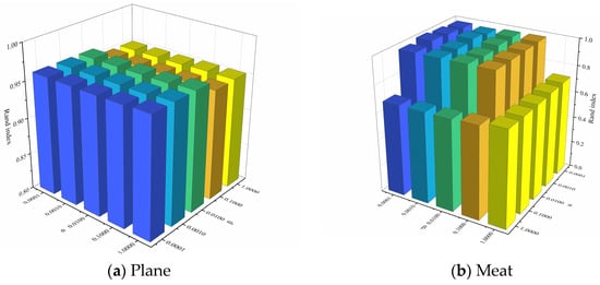
Figure 8.
The effect of changes in and on the clustering performance when k is a constant value.
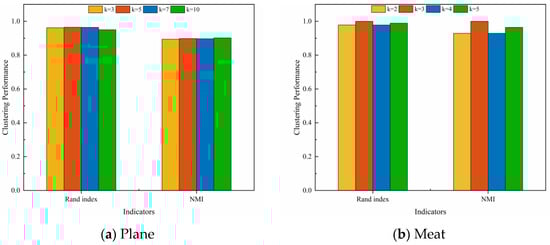
Figure 9.
The effect of changes in k on the clustering performance when and are constant values.
4.3.5. Ablation Experiment
In this section, we set up ablation experiments to analyze the effects of multi-view feature fusion and the contrastive loss function on the clustering performance of the model. The NMI and Rand Index of twelve datasets under different cases are compared, and the obtained experimental results are shown in Table 6.
Table 6.
Comparison of NMI and Rand Index across different cases. (a) Experiments on Coffee, Meat, Herring, and Lightning7. (b) Experiments on DodgerLoopWeekend, ECG200, Plane, and InsectEPGRegularTrain. (c) Experiments on Fish, GunPointOldVersusYoung, ProximalPhalanxOutlineAgeGroup, and EOGHorizontalSignal.
From the experimental results, it can be observed that the model performance is significantly degraded following the removal of network structures, such as the Residual, TCN, and CNN-TCN modules, which are used for multi-view feature fusion. Taking the Coffee dataset as an example, removing the Residual module reduces the NMI from 1.000 in the full model to 0.023, and the Rand Index from 1.000 to 0.501. Removing the TCN module results in an NMI of 0.036 and a Rand Index of 0.507. Removing the CNN-TCN module results in an NMI of 0.600, which is still significantly lower than that of the full model, and a Rand Index of 0.893. This indicates that the multi-view feature fusion mechanism plays a key role in extracting spatial, temporal, and spatial–temporal features of time series data, and the fused complementary information is crucial for enhancing the clustering performance. The absence of any part will lead to difficulty for the model in fully capturing the data features, in turn affecting the clustering performance.
When the contrastive loss function is removed, the model’s performance on each dataset declines dramatically. For example, in the ECG200 dataset, the NMI decreases from 0.352 to 0.129, and the Rand Index decreases from 0.672 to 0.618. In the Meat dataset, the NMI decreases from 1.000 to 0.515, and the Rand Index decreases from 1.000 to 0.708. This fully illustrates that the contrastive loss function plays an indispensable role in enabling the model to learn data features and optimize the clustering structure, effectively promoting intra-cluster compactness and inter-cluster sparsity by adjusting the similarity of positive and negative sample pairs. Without the contrastive loss function, the model cannot accurately distinguish between similar and dissimilar instances, and the quality of clustering is severely impaired.
5. Conclusions
In this paper, we introduce a method, referred to as UCL-TSC, for time series data clustering which effectively solves many challenges faced by traditional methods. The multi-view feature fusion mechanism fully extracts multiple features of the time series data and achieves complementary information fusion through adaptive weight learning, which effectively solves the problem of feature underutilization. By combining the nearest neighbor graph and pseudo-labels to construct positive and negative sample pairs, UCL-TSC accurately captures the intrinsic relationships within the data. The contrastive loss function fuses feature-level, clustering, and regularization terms, allowing the model to better distinguish between similar and dissimilar instances in the clustering process, explicitly optimizing intra-class compactness and inter-class separation, and effectively solving the long-standing problem of fragmentation in the feature space and clustering structure in deep clustering. Experiments on several UCR datasets show that UCL-TSC exhibits good clustering performance on data with different time series lengths, sample sizes, and numbers of clusters, outperforming the other comparative models in terms of Rand Index on most datasets. Hyperparameter experiments verify that the model is robust to hyperparameter selection. The ablation experiments further demonstrate the importance of multi-view feature fusion and contrastive loss functions on model performance.
The ability to effectively cluster time series data demonstrated by UCL-TSC enables it to be better applied in healthcare, industrial IoT, and financial fields. In healthcare settings, UCL-TSC can assist in disease typing or abnormality detection by clustering and analyzing physiological signals. In industrial IoT, UCL-TSC can capture the spatial–temporal patterns of equipment operation, allowing for early failure warning. In future work, we will focus on real-time applications and heterogeneous data fusion to further expand the practical value of this method in emerging fields. Specifically, we will explore online clustering algorithms to improve the model’s usefulness in resource-constrained scenarios. Additionally, we will extend the clustering ability of the model with respect to heterogeneous time series data from multiple sources, so that UCL-TSC can be better applied in different scenarios.
Author Contributions
Resources, L.L.; visualization, X.W.; validation, K.Y.; writing—review and editing, B.C.; supervision, Q.X. All authors have read and agreed to the published version of the manuscript.
Funding
This research was funded by the National Natural Science Foundation of China, grant number 72071209.
Data Availability Statement
The UCR dataset used in the experiments can be obtained from https://www.cs.ucr.edu/~eamonn/time_series_data_2018/ (accessed on 15 February 2025).
Conflicts of Interest
The authors declare no conflicts of interest.
Abbreviations
The following abbreviations are used in this manuscript:
| TSC | Time series data clustering |
| AGNES | Agglomerative nesting algorithm |
| DIANA | Divisive analysis algorithm |
| DBSCAN | Density-based spatial clustering of applications with noise |
| OPTICS | Ordering points to identify the clustering structure |
| HDBSCAN | Hierarchical density-based spatial clustering of applications with noise |
| ARIMA | Autoregressive integral sliding average models |
| DTW | Dynamic time warping |
| UCL-TSC | Unsupervised contrastive learning for time series data clustering |
| TCN | Temporal convolutional neural network |
| CNN | Convolutional neural network |
| ACC | Unsupervised clustering accuracy |
| NMI | Normalized mutual information |
| PUR | Purity |
References
- Vera, J.F.; Angulo, J.M. An MDS-Based Unifying Approach to Time Series K-Means Clustering: Application in the Dynamic Time Warping Framework. Stoch. Environ. Res. Risk Assess. 2023, 37, 4555–4566. [Google Scholar] [CrossRef]
- Huang, X.; Ye, Y.; Xiong, L.; Lau, R.Y.K.; Jiang, N.; Wang, S. Time Series K-Means: A New k-Means Type Smooth Subspace Clustering for Time Series Data. Inf. Sci. 2016, 367–368, 1–13. [Google Scholar] [CrossRef]
- Ozkok, F.O.; Celik, M. A Hybrid Validity Index to Determine K Parameter Value of K-Means Algorithm for Time Series Clustering. Int. J. Inf. Technol. Decis. Mak. 2021, 20, 1615–1636. [Google Scholar] [CrossRef]
- Wang, C.; Zhao, S.; Ren, Z.; Long, Q. Place-Centered Bus Accessibility Time Series Classification with Floating Car Data: An Actual Isochrone and Dynamic Time Warping Distance-Based k-Medoids Method. ISPRS Int. J. Geo-Inf. 2023, 12, 285. [Google Scholar] [CrossRef]
- Li, F.; Wang, C. Develop a Multi-Linear-Trend Fuzzy Information Granule Based Short-Term Time Series Forecasting Model with k-Medoids Clustering. Inf. Sci. 2023, 629, 358–375. [Google Scholar] [CrossRef]
- Dewi, D.A.; Surono, S.; Thinakaran, R.; Nurraihan, A. Hybrid Fuzzy K-Medoids and Cat and Mouse-Based Optimizer for Markov Weighted Fuzzy Time Series. Symmetry 2023, 15, 1477. [Google Scholar] [CrossRef]
- Serra, A.P.; Zárate, L.E. Characterization of Time Series for Analyzing of the Evolution of Time Series Clusters. Expert. Syst. Appl. 2015, 42, 596–611. [Google Scholar] [CrossRef]
- Patnaik, A.K.; Bhuyan, P.K.; Krishna Rao, K.V. Divisive Analysis (DIANA) of Hierarchical Clustering and GPS Data for Level of Service Criteria of Urban Streets. Alex. Eng. J. 2016, 55, 407–418. [Google Scholar] [CrossRef]
- Chang, D.; Ma, Y.; Ding, X. Time Series Clustering Based on Singularity. Int. J. Comput. Commun. Control 2017, 12, 790–802. [Google Scholar] [CrossRef]
- Nicolis, O.; Delgado, L.; Peralta, B.; Díaz, M.; Chiodi, M. Space-Time Clustering of Seismic Events in Chile Using ST-DBSCAN-EV Algorithm. Environ. Ecol. Stat. 2024, 31, 509–536. [Google Scholar] [CrossRef]
- Fu, J.-S.; Liu, Y.; Chao, H.-C. ICA: An Incremental Clustering Algorithm Based on OPTICS. Wirel. Pers. Commun. 2015, 84, 2151–2170. [Google Scholar] [CrossRef]
- Zhao, Y.; Li, H.; Yu, X.; Ma, N.; Yang, T.; Zhou, J. An Independent Central Point OPTICS Clustering Algorithm for Semi-Supervised Outlier Detection of Continuous Glucose Measurements. Biomed. Signal Process. Control 2022, 71, 103196. [Google Scholar] [CrossRef]
- Lee, T.; Kim, Y.; Hyun, Y.; Mo, J.; Yoo, Y. Unsupervised Anomaly Detection Process Using LLE and HDBSCAN by Style-GAN as a Feature Extractor. Int. J. Precis. Eng. Manuf. 2024, 25, 51–63. [Google Scholar] [CrossRef]
- Neto, A.C.A.; Sander, J.; Campello, R.J.G.B.; Nascimento, M.A. Efficient Computation and Visualization of Multiple Density-Based Clustering Hierarchies. IEEE Trans. Knowl. Data Eng. 2021, 33, 3075–3089. [Google Scholar] [CrossRef]
- Péalat, C.; Bouleux, G.; Cheutet, V. Improved Time Series Clustering Based on New Geometric Frameworks. Pattern Recognit. 2022, 124, 108423. [Google Scholar] [CrossRef]
- Zhang, Q.; Wu, J.; Zhang, P.; Long, G.; Zhang, C. Salient Subsequence Learning for Time Series Clustering. IEEE Trans. Pattern Anal. Mach. Intell. 2019, 41, 2193–2207. [Google Scholar] [CrossRef]
- Aslan, S.; Yozgatligil, C.; Iyigun, C. Temporal Clustering of Time Series via Threshold Autoregressive Models: Application to Commodity Prices. Ann. Oper. Res. 2018, 260, 51–77. [Google Scholar] [CrossRef]
- Euán, C.; Ombao, H.; Ortega, J. The Hierarchical Spectral Merger Algorithm: A New Time Series Clustering Procedure. J. Classif. 2018, 35, 71–99. [Google Scholar] [CrossRef]
- Piccardi, C.; Calatroni, L.; Bertoni, F. Clustering Financial Time Series by Network Community Analysis. Int. J. Mod. Phys. C 2011, 22, 35–50. [Google Scholar] [CrossRef]
- Wong, C.; Versace, M. CARTMAP: A Neural Network Method for Automated Feature Selection in Financial Time Series Forecasting. Neural Comput. Appl. 2012, 21, 969–977. [Google Scholar] [CrossRef]
- Javed, A.; Rizzo, D.M.; Lee, B.S.; Gramling, R. Somtimes: Self Organizing Maps for Time Series Clustering and Its Application to Serious Illness Conversations. Data Min. Knowl. Discov. 2024, 38, 813–839. [Google Scholar] [CrossRef] [PubMed]
- Pei, D.; Luo, C.; Liu, X. Financial Trading Decisions Based on Deep Fuzzy Self-Organizing Map. Appl. Soft Comput. 2023, 134, 109972. [Google Scholar] [CrossRef]
- Li, Y.; Du, M.; Jiang, X.; Zhang, N. Contrastive Learning-Based Multi-View Clustering for Incomplete Multivariate Time Series. Inf. Fusion. 2025, 117, 102812. [Google Scholar] [CrossRef]
- Moradinasab, N.; Sharma, S.; Bar-Yoseph, R.; Radom-Aizik, S.; Bilchick, K.C.; Cooper, D.M.; Weltman, A.; Brown, D.E. Universal Representation Learning for Multivariate Time Series Using the Instance-Level and Cluster-Level Supervised Contrastive Learning. Data Min. Knowl. Discov. 2024, 38, 1493–1519. [Google Scholar] [CrossRef] [PubMed]
- Zhong, Y.; Huang, D.; Wang, C.-D. Deep Temporal Contrastive Clustering. Neural Process Lett. 2023, 55, 7869–7885. [Google Scholar] [CrossRef]
- Liu, Z.; Alavi, A.; Li, M.; Zhang, X. Self-Supervised Contrastive Learning for Medical Time Series: A Systematic Review. Sensors 2023, 23, 4221. [Google Scholar] [CrossRef]
- Yang, Z.; Li, H.; Tuo, X.; Li, L.; Wen, J. Unsupervised Clustering of Microseismic Signals Using a Contrastive Learning Model. IEEE Trans. Geosci. Remote Sens. 2023, 61, 5903212. [Google Scholar] [CrossRef]
- Liang, Z.; Liang, C.; Liang, Z.; Wang, H.; Zheng, B. TimeCSL: Unsupervised Contrastive Learning of General Shapelets for Explorable Time Series Analysis. Proc. VLDB Endow. 2024, 17, 4489–4492. [Google Scholar] [CrossRef]
- Alqahtani, A.; Ali, M.; Xie, X.; Jones, M.W. Deep Time-Series Clustering: A Review. Electronics 2021, 10, 3001. [Google Scholar] [CrossRef]
- Özgül, O.F.; Bardak, B.; Tan, M. A Convolutional Deep Clustering Framework for Gene Expression Time Series. IEEE/ACM Trans. Comput. Biol. Bioinform. 2021, 18, 2198–2207. [Google Scholar] [CrossRef]
- Kim, J.; Moon, N. A Deep Bidirectional Similarity Learning Model Using Dimensional Reduction for Multivariate Time Series Clustering. Multimed. Tools Appl. 2021, 80, 34269–34281. [Google Scholar] [CrossRef]
- Li, X.; Xi, W.; Lin, J. Randomnet: Clustering Time Series Using Untrained Deep Neural Networks. Data Min. Knowl. Discov. 2024, 38, 3473–3502. [Google Scholar] [CrossRef]
- He, D.; Tang, Z.; Chen, Q.; Han, Z.; Zhao, D.; Sun, F. A Two-Stage Deep Graph Clustering Method for Identifying the Evolutionary Patterns of the Time Series of Animation View Counts. Inf. Sci. 2023, 642, 119155. [Google Scholar] [CrossRef]
- Cui, J.; Li, Y.; Huang, H.; Wen, J. Dual Contrast-Driven Deep Multi-View Clustering. IEEE Trans. Image Process. 2024, 33, 4753–4764. [Google Scholar] [CrossRef]
- Yeh, C.-H.; Hong, C.-Y.; Hsu, Y.-C.; Liu, T.-L.; Chen, Y.; LeCun, Y. Decoupled Contrastive Learning. In European Conference on Computer Vision; Springer Nature: Cham, Switzerland, 2022; pp. 668–684. [Google Scholar]
- Yang, J.; Leskovec, J. Patterns of Temporal Variation in Online Media. In Proceedings of the Fourth ACM International Conference on Web Search and Data Mining, Hong Kong, China, 9–12 February 2011; Association for Computing Machinery: New York, NY, USA, 2011; pp. 177–186. [Google Scholar]
- Paparrizos, J.; Gravano, L. K-Shape: Efficient and Accurate Clustering of Time Series. SIGMOD Rec. 2016, 45, 69–76. [Google Scholar] [CrossRef]
- Li, X.; Lin, J.; Zhao, L. Linear Time Complexity Time Series Clustering with Symbolic Pattern Forest. In Proceedings of the 28th International Joint Conference on Artificial Intelligence, Macao, China, 10–16 August 2019; AAAI Press: Macao, China, 2019; pp. 2930–2936. [Google Scholar]
- Lei, Q.; Yi, J.; Vaculin, R.; Wu, L.; Dhillon, I.S. Similarity Preserving Representation Learning for Time Series Clustering. In Proceedings of the 28th International Joint Conference on Artificial Intelligence, Macao, China, 10–16 August 2019; AAAI Press: Macao, China, 2019; pp. 2845–2851. [Google Scholar]
- Petitjean, F.; Ketterlin, A.; Gançarski, P. A Global Averaging Method for Dynamic Time Warping, with Applications to Clustering. Pattern Recognit. 2011, 44, 678–693. [Google Scholar] [CrossRef]
- Guo, X.; Gao, L.; Liu, X.; Yin, J. Improved Deep Embedded Clustering with Local Structure Preservation. In Proceedings of the 26th International Joint Conference on Artificial Intelligence, Melbourne, Australia, 19–25 August 2017; AAAI Press: Melbourne, Australia, 2017; pp. 1753–1759. [Google Scholar]
- Madiraju, N.; Sadat, S.M.; Fisher, D.; Karimabadi, H. Deep Temporal Clustering: Fully Unsupervised Learning of Time-Domain Features. arXiv 2018, arXiv:1802.01059. [Google Scholar]
- Dempster, A.; Schmidt, D.F.; Webb, G.I. MiniRocket: A Very Fast (Almost) Deterministic Transform for Time Series Classification. In Proceedings of the 27th ACM SIGKDD Conference on Knowledge Discovery & Data Mining, Singapore, 14–18 August 2021; Association for Computing Machinery: New York, NY, USA, 2021; pp. 248–257. [Google Scholar]


Disclaimer/Publisher’s Note: The statements, opinions and data contained in all publications are solely those of the individual author(s) and contributor(s) and not of MDPI and/or the editor(s). MDPI and/or the editor(s) disclaim responsibility for any injury to people or property resulting from any ideas, methods, instructions or products referred to in the content. |
© 2025 by the authors. Licensee MDPI, Basel, Switzerland. This article is an open access article distributed under the terms and conditions of the Creative Commons Attribution (CC BY) license (https://creativecommons.org/licenses/by/4.0/).