Abstract
Integrating causal inference and estimation methods, especially in Natural Language Processsing (NLP), is essential to improve interpretability and robustness in deep learning (DL) models. The objectives are to present the IV-NLP methodology and its application. IV-NLP integrates two approaches. The first defines the process of the inference and estimation of the causal effect in original, predicted, and synthetic data. The second one includes a validation method of the results obtained by the selected Large-Language Model (LLM). IV-NLP proposes to use synthetic data in predictive tasks only if the causal effect pattern of the synthetic data is aligned with the causal effect pattern of the original data. DL models, the Instrumental Variable (IV) method, statistical methods, and GPT-3.5-turbo-0125 were used for its application, including an intervention method using a variation of the Retrieval-Augmented Generation (RAG) technique. Our findings reveal notable discrepancies between the original and synthetic data, highlighting that the synthetic data do not fully capture the underlying causal effect patterns of the original data, evidencing homogeneity and low diversity in the synthetic data. Interestingly, when evaluating the causal effect in the predictions made by our three best DL models, it was verified that the model with the lowest accuracy (84.50%) was fully aligned with the overall causal effect pattern. These results demonstrate the potential of integrating DL and LLM models with causal inference methods.
1. Introduction
Over the past five years, research has gradually increased on mitigating the limitations in interpreting and explaining the results of AI models using a causal approach. Within this framework, ref. [1] argue that to interpret the results of most machine learning (ML) algorithms, it is necessary to go beyond the famous black box nature of most ML models. Likewise, the models based on deep learning (DL) have proven to be highly effective in predictive tasks in areas such as Natural Language Processing (NLP) and computer vision; however, their dependence on correlations observed in the data makes them susceptible to generating spurious associations, compromising their generalization and explainability [2]. In this sense, the correlations found by most AI models are insufficient to explain causal relationships (Indirect interactions between variables may be considered. Multiple variables may influence a target variable. Possible biases in the synthetic data are also included. In any case, incorrect correlations could be generated between variables, making their interpretation difficult). This literature review is organized into the following thematic subsections:
1.1. Causal Inference in NLP
In this regard, ref. [3] emphasizes that causal relationships are not always evident in the observed data because causality cannot be directly inferred from the observed correlations. The models used for NLP are not immune to this reality, making it necessary to explain the results of a model based on DL. This is a complex task requiring the application of causal inference methods. Yang, J., Han and S.C., Poon, J. [4] state that extracting causal relationships in texts is challenging because causality can be expressed explicitly, implicitly, or inter-sententially (Explicit causality is observed when text markers define the cause–effect relationship. The expression is implicit when the cause–effect relationship can be inferred through knowledge of the context of the study. Inter-sentence causality is when the causal relationship is attributed in several sentences of the text). This leads to causal inference techniques being used to identify underlying causal structures in the data. In this regard, ref. [5] mentions that a particular advantage of causal methodology is that it forces professionals to explain their assumptions, and analyzing their data using causal reasoning will allow them to improve the scientific level of the NLP community. This could improve our understanding of the language and the models we build to process it. Furthermore, ref. [6] claims that DL models ignore intrinsic causal relationships, reducing the precision and robustness of the model’s discernment and preventing its generalization across different domains. We consider that it is necessary to conduct further research on the fusion of the DL models with causal inference techniques to not only ensure precision and robustness but also to obtain the explainability power of the models. For ref. [2], the issues machine learning faces, such as ignoring interventions in the data, domain changes, and the temporal structure of data, must be addressed within a causal framework. The causal approach allows us to understand the cause–effect relationships that go beyond the observed correlations in more depth, thus increasing the robustness of the model. The causal approach favors the generalization of the models; that is, their adaptation to new and different domains. Research has also been conducted on how causal inference techniques can help with the domain shift problem. In this line, ref. [7] compared the performance of domain adaptation methods using structural causal models (SCM), emphasizing how the causal framework can improve cross-domain adaptation.
1.2. Instrumental Variable Method
There are several methods and techniques of causal inference. One of them is the Instrumental Variable (IV) method, which is used to obtain consistent estimates of the effect of an explanatory variable on a dependent variable; that is, it is applicable when there is endogeneity in the explanatory variable. Along these lines, ref. [8] argued that the F statistic and the partial R2 at the first stage are essential indicators to validate the quality of the instrument. Likewise, it is required that the instrument used meets the criteria of relevance and exogeneity. Angrist, J. and Imbens, G [9] argued that combining a valid instrument and a condition regarding its relationship with the explanatory variable is sufficient to identify the causal effect. Molak, A. and Jaokar, A. C. [10] state that the IV method is a family of techniques that mitigate the bias between variables. Along these lines, we could say that they help reduce the risk of generating erroneous associations between variables.
1.3. Synthetic Data Generation
Social networks facilitate user discussions regarding sociopolitical phenomena in their country. However, the current security and privacy policies restrict access to this type of information. Considering this, Generative Artificial Intelligence (GAI) models represent a potential alternative to increase the amount of data. Lu et al. [11] argue that when faced with the scarcity of quality data and difficulties in accessing data due to privacy and regulatory issues, synthetic data generation can facilitate access to data that the real world cannot offer. Large Language Model (LLM) models have transformed multiple areas of NLP, from text generation to assistance in specialized tasks within this field. Studies have been conducted to integrate new information into LLMs using techniques such as Retrieval-Augmented Generation (RAG). RAG combines generative models with external information retrieval to improve the accuracy of the generated responses. Lewis, P. [12] introduced this approach to tackle knowledge-intensive tasks, showing that the combination of generation and retrieval can mitigate some inherent limitations, such as the possible generation of false synthetics. On the other hand, authors such as [13] disagree with the concept of “hallucinations”, suggesting that models such as GPT incorrectly perceive reality because they are not designed to represent the truth but to generate text that sounds coherent and plausible, regardless of its relationship to reality. The OpenAI white paper on GPT-4 [14] documents the capabilities and limitations of these models, noting that while they can generate highly coherent text, they still face issues related to the veracity of their responses. This supports the idea that LLMs are not designed to present guaranteed facts but to generate plausible text based on the patterns identified during their training.
Considering these issues, this research questions the common approach of selecting models based solely on their performance on unseen data. It seeks to answer the following research question: Why is it important to determine the pattern of causal effects in the predicted data to determine which model best fits reality? Furthermore, our research demonstrates that validating the results provided by an LLM is necessary. Likewise, we demonstrates that synthetic data are not ideal for capturing causal patterns. Therefore, we aim to answer the following question: Why is it necessary to include causal inference techniques to evaluate the behavior of data generated by an LLM from a causal perspective? To answer these questions, this paper proposes the IV-NLP methodology and develops an application of the proposed methodology. The IV-NLP methodology defines a flexible action path to apply inference and causal effect estimation methods to original, synthetic, and predicted data. IV-NLP includes a validation method for the data the selected LLM generates. Two approaches are integrated to address these challenges. A method is introduced to implement causal inference using the IV method on original, synthetic, and predicted data, and a validation method is proposed for generating text using an LLM.
For its application, the DL models used in binary classification problems in the field of NLP, the Instrumental Variable (IV) method, and statistical methods were used to determine and calculate causal inference and estimation. To determine the pattern of the causal effect in the original data set, the synthetic data, and the predicted data, a method to implement causal inference through the use of the IV method was designed and implemented to analyze, understand, question, and explain the predictions that the DL models provided regarding the detection of argumentative texts in Spanish to explain and interpret the results that the models provided from a causal approach. In this regard, unlike approaches where the validity of the IVs is justified only with narrative arguments, in this research, a rigorous identification was carried out, since its relevance and compliance with the exclusion restriction were demonstrated through regression and statistical models. To verify and evaluate the results of an LLM, a validation method for text generation was designed and implemented using the GPT-3.5-turbo-0125 model. This method used the original data set and the recovery of textual files, regarding the study domain as a variation of the RAG technique. This was carried out to mitigate possible incidents regarding the generation of “synthetic fakes” and validate the quality of the generated synthetic data. Regarding the predictive tasks, various DL models were implemented, and the three best models (CNN, CNN-LSTM-MLP, and CNN-LSTM-MLP, with automatic saving during training) were selected based on their performance on unseen data. Three predicted data sets were obtained. Finally, the evaluation and explanation of the results provided by the three best DL models was carried out using a causal approach. The most important findings were as follows: the best model (85.82% performance on new data) significantly deviated from the estimated overall causal effect; the third-best DL model (84.50% performance on new data) was completely aligned with the overall causal effect estimated with the original data; although the intervention method for generating texts using GPT-3.5-turbo-0125 significantly mitigated the generation of false synthetics, low quality was evident in the synthetic data generated by GPT-3.5-turbo-0125 due to the homogeneity of the generated words and its limitations in the context of specific domains, which made its interpretation and analysis difficult.
This research seeks to improve the ability to understand DL models using a causal approach and expose the need to validate the results provided by an LLM and evaluate them from a causal perspective. The convergence between the causal-focused methods, DL and LLM, represents an expanding line of research with direct implications for the robustness and interpretability of AI models in NLP applications. In summary, our findings highlight the potential of integrating causal inference and estimation methods into DL models in the field of NLP and the need to apply methods that include the verification and validation of data generated by LLMs regardless of the study domain in which they are applied.
2. Related Work
2.1. Causal Inference
In this context, approaches incorporating causal inference have emerged to improve the robustness of these models. Wu et al. [15] argue that causal inference uses assumptions, study designs, and estimation strategies to determine the causal relationships between variables based on data to understand better how complex systems work and support decision-making. Along these lines, several studies have explored the integration of causal inference in DL models, allowing for the identification of the underlying causal relationships in the data and improving the stability of the models [16]. Sui et al. [17] introduce the concept of Causal Attention, a method that improves the interpretability of graph classification models by eliminating the effects of confounding variables. This approach allows models to learn optimal representations and be more explainable and generalizable in structured classification tasks. Similarly, ref. [18] explores the use of causal representation learning from multimodal data in biology, demonstrating how causal inference can identify spurious correlations through causal techniques, allowing models to learn representations that are more faithful to the underlying relationships in the data. Addiitonally, ref. [5] argues that one of the techniques that can be used to implement a causal method regarding the results provided by DL models is causal formalisms based on the generation of “Counterfactual” component. These represent statements that would be true under different circumstances. Counterfactuals can be considered hypothetical or simulated interventions that assume a particular situation, for example, “I would have arrived at the office on time if I had taken the train instead of the car” [10]. Ref. [19] analyzed the work that has been carried out, categorizing it into two groups: a group of studies using evidence-based data seeking statistical causal inference, and a second group of studies without causality objectives that prioritize prediction. Much of this research has not emphasized the need to enhance the explanatory and interpretive capacity of DL models but instead prioritized mitigating the presence of spurious correlations and improving performance metrics and model robustness. Our research questions the notion that the best model can be selected based primarily on its predictive capacity. Our work seeks to balance model performance and its explanatory and interpretive capacity from a causal perspective in NLP.
2.2. Instrumental Variable Method
Pearl, J. [20] defined three types of causal methods, one of them being the IV, which cannot be identified either directly or from its constituents (it has none), but can be determined from the effect that Z (the variable that plays the role of the instrument) has on Y (the independent variable) and Z on X (the dependent variable). The IV method significantly mitigates the endogeneity of the variables [21]. Martens et al. [22] defined three requirements for the validity of an IV: relevance, exclusion, and independence of error. Authors such as those of refs. [23,24,25] grouped the last two requirements under the concept of exogeneity. Likewise, ref. [15] present a comprehensive framework for identifying and estimating causal effects through IVs, addressing both traditional approaches and recent methods based on ML. According to ref. [26], the IV method facilitates the distribution of treatment through a procedure where, in the first stage, the treatment is applied, and in the second stage, counterfactual predictions are made. On the other hand, in low-dimensional contexts, the data sets often do not explicitly include a clearly defined treatment variable. However, an in-depth understanding of the domain under study allows us to infer which variable can serve as an instrument. The IV method addresses this challenge by identifying the causal relationships, provided the selected instrument meets the fundamental criteria of relevance and validity. Our approach has proven very useful when treatment assignments are not directly observed but can be inferred through an appropriate instrument. This study used the IV method to apply the causal approach to pre-trained DL models, highlighting its usefulness in data settings with a limited structure.
2.3. Synthetic Data Generation in NLP
He et al. [27] proposed the use of the GAL method to generate synthetic data using the GPT-2.0 model, annotate those data with pseudo-labels generated by classifiers, and learn through combining real data with synthetic data to mitigate the sparsity of specific data points and improve the performance of the models. Yang et al. [28] proposed G-DAUG, a data generation method using the GPT-2.0 model to improve common-sense reasoning in the field of NLP by applying a two-stage training selection process to promote the diversity of the data added to the training and consequently improve the quality of the data. Ref. [29] analyzed the effectiveness of the GPT-3.5-turbo model for data generation. In this regard, the performance of the models trained with this synthetic data (where, using the few-shot approach, real data are used as a guide in generating data) for text classification tasks was close to that of the models trained with real data. LLMs acquire their knowledge during the training stage. However, they are challenging to interpret because they cannot yet emulate the structured reasoning of a traditional knowledge base [30]. This translates into the need to analyze and evaluate the results of an LLM using a causal approach to verify whether the data generated are aligned with the reality of the context or simply generate coherent, understandable ideas or biases without necessarily being aligned with the real context. In this regard, recent findings by ref. [31] warn that incorporating new knowledge through fine-tuning in large language models (LLMs) can increase the model’s propensity to generate incorrect or “hallucinated” answers, especially when dealing with information that is not part of its pre-trained knowledge. In contrast to this approach, the present work adopted a strategy based on a variation of the standard RAG by incorporating text files containing domain-specific knowledge. While this technique does not modify the model’s parameters, it also faces limitations since its ability to generate expected results depends on adequate context structuring and the input window limits. This methodological difference highlights a common challenge: the difficulty of integrating new knowledge that has not been pre-trained into the LLMs. Therefore, our findings reinforce what ref. [31] established because we expose the current limitations in LLMs when adapted to a specific domain.
3. Methodology
The IV-NLP methodology is proposed in Figure 1. IV-NLP represents a general-level methodology, ignoring technical details such as methods, techniques, AI models, statistical models, and specific technological tools for its implementation. IV-NLP proposes two approaches for its application:

Figure 1.
IV-NLP methodology.
3.1. First Approach
This approach defines the inference and estimation of the causal effect on original data, predicted data, and optionally, synthetic data. Yao L. et al. [16] argue that causal inference is the process of concluding a causal connection based on an analysis of the response of the effect variable when the cause changes. Along these lines, we can state that causal inference validates whether a causal relationship exists between variables and provides statistical evidence of that relationship. Causal estimation quantifies the statistical evidence of the causal effect of the treatment variable on the outcome. Likewise, this approach addresses the claim by ref. [6] that DL models ignore intrinsic causal relationships, thereby diminishing the accuracy and robustness of the model. IV-NLP exposes the intrinsic causal relationships of DL models to identify the cause–effect pattern of the results obtained with DL models. Likewise, in line with ref. [32], the IV-NLP methodology requires an explanation of the results and analyzes the data using a causal approach, which will allow for the scientific level of the NLP community to be improved. IV-NLP analyzes and evaluates the overall causal effect pattern of the data set. Subsequently, it trains AI models to obtain the best models based on their performance metrics on unseen data and generates the predicted data sets. Next, it estimates the causal effect on the predicted data and compares the overall causal effect pattern with the causal effect pattern on predicted data to interpret and explain these results using a causal approach.
3.2. Second Approach
IV-NLP includes the generation of synthetic data as an alternative to augmented data but includes a method of validating the results obtained by the selected LLM. Note that IV-NLP proposes that, regardless of the LLM used, a method of validating the results obtained (automated and/or manual) must be included to mitigate the problem of biases, false synthetics, or inconsistencies in the responses. However, this does not solve the problem. Zhou et al. [33] argue that there is a need for a fundamental change in the design and development of general-purpose artificial intelligence, particularly in high-risk areas for which a predictable distribution of errors is essential. Likewise, IV-NLP proposes using a synthetic data set for predictive tasks only if the pattern of the causal effect of the synthetic data aligns with the pattern of the causal effect of the original data. This could evaluate whether the pattern of causal effects in the synthetic data aligns with the real-life context of the original data. This is extremely important because before using synthetic data in predictive tasks, their consistency with reality must be assessed. In the Application section, each process diagrammed in Figure 1 is presented in detail.
4. Application
The application of the IV-NLP methodology is presented below. The classification of argumentative and non-argumentative texts in Spanish on the sociopolitical events in Peru between 2020 and 2021 was taken as a case study.
4.1. Data Preparation
The data preparation stage is crucial to generating quality results in line with the context of the reality from which they were obtained (Twitter, now X). Engineering tasks were carried out to prepare and process the original data, synthetic data, and recovered data, the latter with the purpose of providing greater context to the data set and enhancing its use during the analysis and evaluation stage of the causal effect pattern in the data.
4.1.1. Original Data
The data set was generated from a corpus of 4000 records used to propose and evaluate an annotation method for argumentative and non-argumentative texts in Spanish [34]. The previously published corpus for the detection of argumentation in Spanish, corresponding to the first annotation task, is available in Mendeley Data (Mendeley Data Repository: https://data.mendeley.com/datasets/xh7vvty9zt/3 (accessed on 6 June 2023)) and contains 2875 texts annotated as Argument or Non_Argument (1 and 0, respectively). Subsequently, a review of 1125 labeled records was carried out to guarantee the reliability of the data. The 4000 records were extracted from the social network Twitter (2021), covering the period 2020 and 2021 during the general elections in Peru. Next, 15 records extracted from the Portal of the Constituent Process at the Service of the Peoples of Peru [35] were added. In total, 4015 records labeled in Spanish were obtained (Mendeley Data Repository: https://data.mendeley.com/datasets/rcn3swj868/2 (accessed on 7 April 2025)). Finally, the original data were distributed (training, testing, and validation). Likewise, a sub-subset of argumentative and non-argumentative texts was distributed for each data subset to preserve the class balance during the data preparation stage.
The data set was divided into training, testing, and validation sets. This was achieved using a special function to automatically distribute the data to ensure a balanced distribution of the argument and non-argument classes. No data were subtracted for validation from the training set, although this is frequently done. The data set was distributed referencing the work of [36], in which the training, testing, and validation sets represent 78%, 17%, and 5% of the total records in the data set. Likewise, the distribution kept the data balanced (Table 1). The training and validation sets were used to train and adjust the ML models, respectively, while the testing set was used to evaluate the final performance of the ML models with the untrained data to ensure an unbiased evaluation of the ML models was achieved.

Table 1.
Data distribution.
4.1.2. Synthetic Data
For the case study used in the application of IV-NLP, it was necessary to generate synthetic data from the real data due to the limitations in accessing Spanish text in the context of the study’s subject and to make modifications to the original text in order to carry out the intervention on the [20] ladder and subsequently verify how this influences the target variable. Because this research work began in 2023, different GPT 3.5 models were experimented with, as follows.
The “gpt-3.5-turbo-0125” model handles a limit of 250,000 tokens per minute (TPM), which is why better results were obtained; that is, the results were acceptable for the objectives pursued in this research. Some adaptations and resources were implemented in the configuration of the “chat.completions.create” library of the “gpt-3.5-turbo-0125 model”, such as the design and implementation of a file of discourse markers in Spanish, a file containing a list of authorities, the size of the generated text, the configuration of the text generation stop, and the level of creativity and coherence, among others. The file containing the list of authorities represents an ‘Authority,’ so in the political context of a State, a statement, report, or report issued by the competent authority can be considered an argumentative text. For example, a presidential candidate is not an authority, but the PNP (National Police of Peru) is an institution that represents authority in the country. Regarding the text stop configuration, a modification was made to the max_tokens=250 parameters and the stop=[“.”] parameter was not used; instead, the task of the “content” variable of the “system” role of the gpt-3.5-turbo-0125 model was modified, emphasizing that the generated sentences should be terminated with a period to offer the model freedom during the text generation process. To carry out the validation method proposed in IV-NLP (Figure 1) for the output of an LLM, the following phases were designed and implemented (Figure 2):
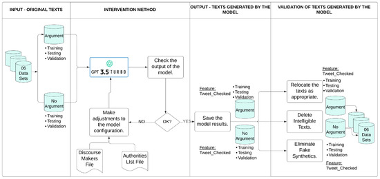
Figure 2.
Validation method for text generation using the “GPT-3.5-turbo-0125” model.
- Input—Original texts: Six (06) data subsets were generated, including argumentative and non-argumentative texts for each training, test, and validation data set. A small sample of each data subset was selected to ensure that the results generated by the GPT-3.5-turbo-0125 model responded to the research needs.
- Intervention Method: An iterative process of adjustments, modifications, and improvements to the model was carried out to achieve results that were acceptable regarding the study’s objectives. These adjustments included parameter adjustment, the elaboration of specific inputs with precise examples to provide context to the model, rules to specify the end of the generated sentence, and the specific configuration of the parameters temperature, max_tokens, and stop. A variation of the standard RAG (Retrieval-Augmented Generation) technique was implemented. Text documents were created as discourse markers, providing a list of authorities to introduce new information and mitigate the generation of false synthetics that the model could eventually generate. This process was repeated as often as necessary until acceptable results were achieved.
- Output—texts generated by the model: The results generated by the model were saved.
- Validation of texts generated by the model: Each time errors were identified during the validation of the results produced by the model for each of the six (06) data sets, the records in the data set were relocated (if the text generated by the model was incorrect, meaning the model generated a non-argumentative text when it should have generated an argumentative text and vice versa) and/or eliminated (if the text generated by the model was intelligible, contained up to five tokens, or was a synthetic false text, then it was eliminated to avoid manipulating the data and avoid possible biases). This method was chosen not only to rationally and efficiently use all the records in the data sets but also to calculate the expected value of the counterfactual for the intervention that was carried out. Finally, the argumentative and non-argumentative records correctly generated by the model for each of the six (06) data sets were totaled.
The first result after implementing the GPT-3.5-turbo-0125 model for each of the six (06) data sets in the OUTPUT stage—TEXTS GENERATED BY GPT-3.5-turbo-0125 of the Intervention Method (Figure 2):
The generated records were the synthetic texts generated by the model without any validation (intervention method’s output stage), while the correctly generated records were the synthetic texts correctly identified as argumentative and non-argumentative texts. The first results obtained are displayed in Table 2:
Table 2.
First results generated during the OUTPUT stage—TEXTS GENERATED BY GPT-3.5-turbo-0125 of the proposed intervention method (Figure 2).
The second result after having concluded the validation stage of the results generated by the intervention method (Figure 2) using the GPT-35-turbo-0125 model:
The correctly generated records were the synthetic texts that were reassigned or relocated to the category of argumentative or non-argumentative texts, as appropriate, at the end of the intervention method’s validation stage. The results obtained are displayed in Table 3.
Table 3.
The second result was generated at the end of the VALIDATION OF GENERATED TEXTS stage, which was proposed by the intervention method using GPT-3.5-turbo-0125 (Figure 2).
4.1.3. Recovering Features from Original and Synthetic Data Sets
It was necessary to recover characteristics from the data set (described in the data in item a. Original Data of Section 4.1, Data Preparation) that allow for the design and implementation of a method and/or technique that responds to the inference or causal formalisms that will enable the interpretation and explanation of the results obtained. Due to the effort and cost of increasing the characteristics in the original and synthetic data set that ensure the robustness and consistency of the data, Appendix A provides more granular information about this process.
The results of this process are presented in Table 4. Finally, a synthetic data set was obtained, with 3966 generated and validated records. (Mendeley Data Repository: https://data.mendeley.com/datasets/rcn3swj868/2 (accessed on 7 April 2025)). Its features are Id (automatic sequential from 0 to 3965), Tweet_Checked (Text), Original_Id (Id that corresponds to the original data), Date, and Class_Argument.
Table 4.
The results are detailed at the end of Step 3, and the second result is shown in Table 3.
4.2. Deep Learning (DL) Models
To apply the IV-NLP methodology (Figure 1), during the training phase of the DL models, it was exceptionally necessary to retrain the three best models because, during training, the predicted data sets that are necessary for their subsequent evaluation concerning the global causal effect pattern were not generated. Therefore, it is recommended that, to apply IV-NLP in another case study, the predicted data sets of the best DL models be generated at the end of training.
4.2.1. Training DL Models with Original Data
The data sets were distributed according to Table 1 to ensure the model adequately generalizes the data not used during the training stage (test set). The objective of this phase is to evaluate the performance of the results obtained using the classification models based on the estimation of the global causal effect. It will be possible to evaluate whether the model can classify the texts according to a pattern reflecting the estimated causal relationships, thereby verifying whether the DL models align or deviate from the estimated causal effect structure.
Models based on conventional neural networks were chosen due to their lower architectural complexity and greater ability to explain and interpret causal analysis. Following ref. [16], machine learning and causal inference can enhance each other. Therefore, more controllable neural network architectures were chosen to explain this mutual support. During this phase, the following DL models were first trained: LSTM, CuDNNLSTM, Bidirectional CuDNNLSTM, CNN, CNN-LSTM, and CNN-LSTM-MLP. For the LSTM and CuDNNLSTM models, the following hyperparameters were employed: batch_size = 256, callbacks using EarlyStopping, epochs = 30, and Adam optimizer. The same hyperparameters were used for the Bidirectional CuDNNLSTM model, but with an epoch of 25.
Since the data are Spanish texts, the Glove embeddings of SBWC (Spanish Billion Word Corpus) were used, for which the pre-trained vectors in Spanish were downloaded and loaded with the following configuration: 2B tweets, 27B tokens, 1.2M vocab, uncased, 200d vectors, and 1.42 GB for the models to semantically learn the textual content. The results of the DL models CNN, CNN-LSTM, and CNN-LSTM-MLP, using the testing set, are presented below (Table 5). A batch_size of 256 was considered, an EarlyStoppping with Patience = 5 trained in 25 epochs, and Glove SBWC with dimension vectors 200 for the Embedding layer. Furthermore, the SBWC Glove embeddings yielded 1761 words as part of the OOV, out of a total of 60,000, representing approximately 2.9% of the total, which is acceptable for most NLP works. Also, the CNN, CNN-LSTM, and CNN-LSTM-MLP models usually adequately improve OOV terms due to their generalization ability.
Table 5.
DL models with the first results.
4.2.2. Generating Predicted Data Set to Assess the Causal Effect
To ensure consistency and, above all, reproducibility in the retraining process for the selected models, the random seed was set to 42 in the following libraries: random.seed(42), np.random.seed(42), and tf.random.set_set(42). This made it easier to keep the initialization of weights consistent so that any internal operation involving randomness in TensorFlow (version 2.17.1)/Keras (version 3.5.0) remained relatively controlled. It should be noted that the original data sets with recovered features (item c. of Section 4.1.3, Recovering Features from Original and Synthetic Data Sets) were used in order not only to add context to the results of the DL models that were not previously considered in the training stage but to apply and estimate the causal effect through the IV method.
For the CNN and CNN-LSTM models, the same training configuration was maintained because better results were obtained from the experiments performed. Regarding the hybrid CNN-LSTM-MLP model, the “Cyclical Learning Rate” method was implemented through the “LearningRateScheduler” library of the Keras framework. The retraining process was documented in a Github repository (https://github.com/YudiGuzman/Retraining_IV-NLP (accessed on 3 April 2025)) An additional callback was implemented to save the best model obtained during training. Likewise, the predicted sets were generated using the models with the best performance in terms of test_accuracy. Additionally, for the best model (CNN-LSTM-MLP), predicted sets were generated for the model with which the retraining stage ended and for the best model obtained during the retraining stage. After completing the retraining process, the three best models obtained were the following: CNN, CNN-LSTM-MLP (using the CLR method), and CNN-LSTM-MLP (using the CLR method with automatic saving). The architecture of the best model is described in detail in Section 5.2.1. of Section 5, Behaivor and Performance of the Best Model.
Finally, the three corresponding predicted data sets were generated once the three best models were selected through the DL model’s retraining. This allowed us to evaluate how the quality of the model affects the estimation of the causal effect, since the best model will not necessarily produce more precise causal estimates as this will depend on how its predictions interact with the original data.
4.3. Causal Inference Pipeline Using the IV Method
Figure 3 graphically represents the application of the first approach of the IV-NLP methodology (Figure 1). In this regard, the IV method was applied to the original data and synthetic data to evaluate the behavior of the causal effect in the synthetic data generated by GPT-3.5-turbo-0125 for the original data. Likewise, the IV method was applied to the predicted data generated by the three best DL models to verify whether the best model from the perspective of performance metrics was better and more naturally aligned with the pattern of the global causal effect.
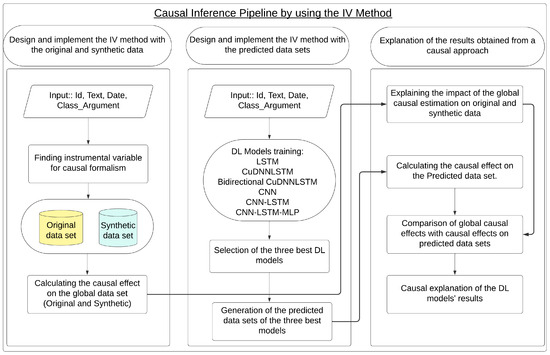
Figure 3.
Causal Inference Pipeline using the IV Method in Original and Synthetic Data and Predicted Data.
4.3.1. Phase 1: Design and Implement the IV Method with the Original Data
Once the process of increasing and/or recovering the characteristics in both the original and synthetic data sets was successfully completed, the instrumented variable method (Instrumental Variable—IV) was implemented to calculate the causal effect of the results achieved. The method that was designed and implemented consists of the following steps:
- Step 1: Selecting the attribute that will fulfil the role of “Instrument”This method will provide an estimate of the causal effect of “Text” on the “Target Class” using the attribute “Date” in this research. This step establishes the publication date’s relevance (pertinence) and exogeneity as an instrumental variable. To demonstrate that the choice of the attribute “Date” as an instrument was correct, it was verified that “Date” as an instrumental variable (Z = Date) meets the following criteria: relevance concerning its correlation with X (X = Text)—that is, Z must have some relation to the content of variable X; and exogeneity, meaning Z must not be correlated with variable Y (Y = Target Class) and that Z must not have a direct effect on Y or be correlated with unobserved factors that influence Y.
- –
- Step 1.a: Data preparation with temporality and topicsTopics were assigned to the texts by time period (every 02 months) based on the publication date. The LDA (Latent Dirichlet Allocation) model was implemented to identify the topics or themes present in the text throughout the study period (2020–2022). Due to the number of records in the data set (4015 instances), 05 topics were defined for evaluation. The topics generated by the model were the following (the first six generated tokens are included):
- *
- Topic 0: elections vote Castillo Keiko second round;
- *
- Topic 1: constituent assembly elections president congress new constitution;
- *
- Topic 2: elections electoral vote onpe security local;
- *
- Topic 3: elections presidential party candidate congress peru;
- *
- Topic 4: elections electoral jne new constitution constituent assembly.
- –
- Step 1.b: Checking the relevance of the publication dateThis section demonstrates that the feature ‘Date’ correlates with the feature ’Tweet_Checked’ (original text). That is, the influence of “Date” on the content of the “original text” is evaluated and verified. A correlation analysis was performed to demonstrate the relevance of “Date” in relation to the content of the topics for which the regression models were implemented where the proportions of the topics were defined as dependent variables and the date (in numerical format) was defined as an independent variable. The regression model used to analyze the impact of “Date” was the OLS (Ordinary Linear Regression) of the “statsmodels” API. The “seaborn” library was used to better visualize the results. Figure 4 shows the results obtained for each topic.
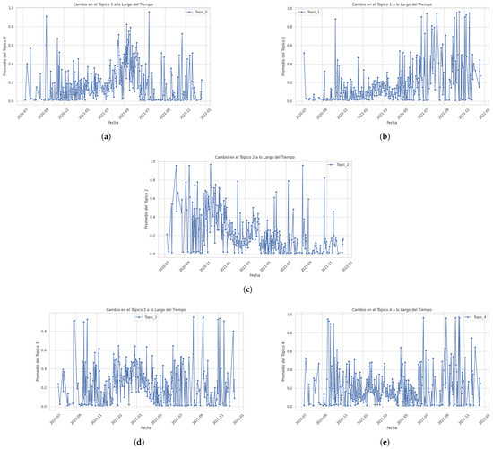 Figure 4. Variation in topics between the period 2020 and 2022: (a) variation in Topic 0; (b) variation in Topic 1; (c) variation in Topic 2; (d) variation in Topic 3; (e) variation in Topic 4.The values shown in Table 6 show that all p-values are less than 0.005, so date has a statistically significant influence on each of the topics; therefore, it was inferred that date is a relevant (pertinent) factor for predicting textual content in terms of the generated topics. Likewise, the coefficient values are small, which could be due to the scale of the date variable. However, the “p” values shown by the F-Statistic parameter indicate that this relationship is robust and reliable. Finally, the R-squared for each topic is low, which indicates that although the Date is significant, it only explains a small fraction of the variability in each topic. This is common in textual analysis, where multiple factors influence the content. In conclusion, it was demonstrated that there are clear differences between the variables studied regarding the variability of each topic analyzed between the years 2020 and 2022, demonstrating the influence of ‘Date’ on ‘Text’.
Table 6. Results obtained to establish the relevance of ‘Date’ as IV.
Figure 4. Variation in topics between the period 2020 and 2022: (a) variation in Topic 0; (b) variation in Topic 1; (c) variation in Topic 2; (d) variation in Topic 3; (e) variation in Topic 4.The values shown in Table 6 show that all p-values are less than 0.005, so date has a statistically significant influence on each of the topics; therefore, it was inferred that date is a relevant (pertinent) factor for predicting textual content in terms of the generated topics. Likewise, the coefficient values are small, which could be due to the scale of the date variable. However, the “p” values shown by the F-Statistic parameter indicate that this relationship is robust and reliable. Finally, the R-squared for each topic is low, which indicates that although the Date is significant, it only explains a small fraction of the variability in each topic. This is common in textual analysis, where multiple factors influence the content. In conclusion, it was demonstrated that there are clear differences between the variables studied regarding the variability of each topic analyzed between the years 2020 and 2022, demonstrating the influence of ‘Date’ on ‘Text’.
Table 6. Results obtained to establish the relevance of ‘Date’ as IV. - –
- Step 1.c: Verify that the publication date has no direct influence on the classThis step shows no correlation between date and class, reinforcing the validity of ‘date’ as an IV. The linear regression of class against date was performed using the OLS model. Table 7 shows the results. The correlation value between ‘date’ and ‘class’ is 0.0833 (Figure 5).
Table 7. Results obtained to establish the exogenity of ‘date’ as IV.
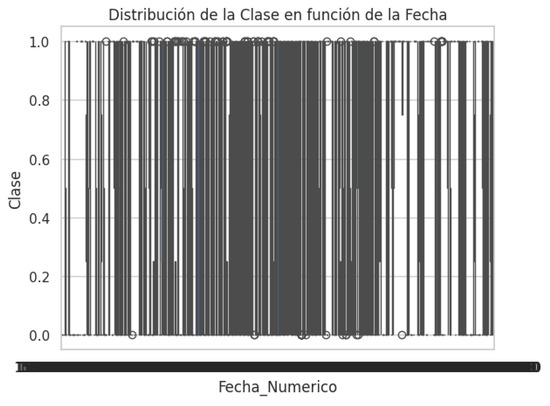 Figure 5. Class distribution for date.The values shown in Table 7 show that the R-squared value indicates that only 7% of the variability in the class variable is explained by the date, which is a very low value and shows that date has no significant relationship with class. On the other hand, F-Statistic has a value of 28.08 with a p-value of , which indicates that, in general terms, the model is significant, but does not imply that date is a good variable to explain class because the R-Squared is too low. The value of the constant is −7.5862, which indicates that when date is 0, the class value is negative, reinforcing the idea that date has neither a positive nor a negative impact on class. Finally, the Durbin–Watson value is 1.792 (close to 2), showing no residual autocorrelation in the model. In conclusion, the date explains virtually none of the variability in the class, as demonstrated by the R-Squared result, so date has no significant effect on class.
- Step 2: Estimating the causal effect using ‘date’ as an instrumental variable (IV)The instrumental regression was performed in the following two (02) steps:
- –
- Step 2.a: Regression of X (topic) on Z (date)This first stage of the regression allows us to estimate the part of X determined by Z. The predictions of this regression are stored in a data frame and are the “instrumented” versions of X; that is, they are free of endogeneity (Table 8).
Table 8. Results obtained to establish the endogeneity of X over Z using an OLS regression model.
- –
- Step 2.b: Regression of Y (class) on instrumented XThe saved predictions (instrumented versions of X) were used to predict Y in a second regression. This provided an unbiased estimate of the causal effect of X on Y. The results are shown in Table 9.
Table 9. Results of the causal effect of Z on Y using ‘Date’ as IV.
- Step 3: The analysis and interpretation of the results in Table 9 is developed in Section 5.1.1, Original Data.
4.3.2. Phase 2: Design and Implement the IV Method with the Synthetic Data
This stage aims to evaluate whether the texts generated by the GPT-35-turbo0125 model maintain the instrumental relationship verified in the original data set to validate the robustness of the causal effect. The topics generated from the synthetic data were as follows:
- Topic 0: constitution constituent assembly new elections fundamental;
- Topic 1: elections fundamental onpe voting guarantee process;
- Topic 2: elections proposals party candidates congress candidate;
- Topic 3: elections peru according to important presidential castle;
- Topic 4: peru elections constituent fundamental important castle.
The steps were the same as those applied to the original data. In Step 1, it was verified that the attribute ’Date’ met the requirements of relevance and exogeneity for the role of the instrument. It is worth mentioning that verifying the exogeneity with the synthetic data generated greater effort because, although the results were significant for the p-value of the coefficients obtained in the model, the Durbin–Watson (DW) value was very close to zero (0) (Table 10) due to the model, so the Logistic Regression (LR) model with HC3 for the robust error type was implemented (Table 11). It should be noted that even though the DW in synthetic data was very low, this does not change the fact that the variable “Date” has no significant influence on “class”. As a result of implementing the LR model, a Pseudo R-squared of 0.005 was obtained. This pseudo R-squared was quite low, indicating that the model does not explain much of the variability of the dependent variable (0 or 1). Although a low pseudo R in logistic models is not unusual, it could be inferred that Date_Numeric_log does not strongly influence class. Therefore, the fact that low R-squared values were obtained in both the linear and logistic regression, and the low impact of date as a predictor variable of class, confirm that date has no significant influence on class (Figure 6); therefore, the variability of class is not explained by the date.
Table 10.
Results obtained to establish the exogeneity of ‘date’ as IV using a linear regression model.
Table 11.
Results obtained to establish the influence of ‘date’ on ‘cass’.
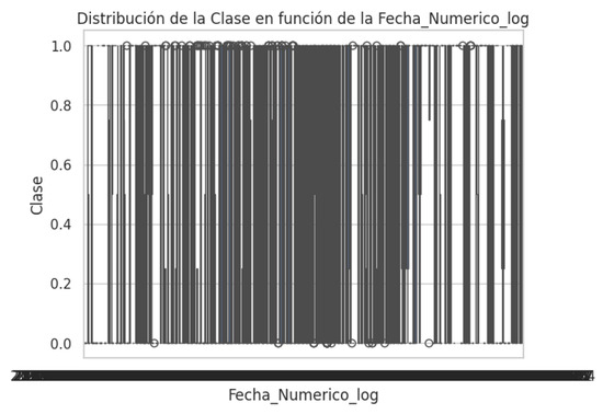
Figure 6.
Class distribution with respect to date.
In Step 2, for the estimation of the causal effect, the first regression of X (synthetic topics) on Z (date) was used; the results were as follows (Table 12).
Table 12.
Results obtained to establish the endogeneity of X over Z using a linear regression model.
Table 12 shows that the R-squared values are low, which indicates that up to 10.7% of the data explain the variability of X and, thus, the influence of “X” on “Z”. Although the results are very significant for the p-value of the coefficients obtained in the model (except for Topic 3), the DW value is very close to two (2), which indicates that there is no autocorrelation in the errors generated by the model, which shows that the model is optimal.
During the second regression of Y (class) on instrumented X, difficulties were experienced due to the limitations of the GT-35-turbo-0125 model in generating quality data. It was quite difficult to determine the best model, which could obtain results that not only converge but also explain the causal effect of the same. At this stage, the following models were implemented:
- The OLS model yielded a very low value (0.019), which indicates a high autocorrelation in the model’s residuals. This represented a potential problem for the validity of the results, i.e., the model could bias the inferences, so it was necessary to experiment with other more robust models to mitigate the problem of autocorrelation of the model’s errors.
- The Logistic Regression (LR) model generated 35 iterations. By exceeding the number of iterations, the model failed to converge towards stable results, so this model did not obtain the expected results either.
- Finally, a robust regression model (RLM) was implemented using the HuberT standard to manage the sensitivity of outliers, which are associated with the quality of the data generated by the GPT-35-turbo-0125 model (Table 13). This choice was based on the model’s ability to balance sensitivity and robustness, its resistance to outliers, the lower complexity in its application in exploratory analyses, and its low computational resource requirements. This technique was originally proposed in 1964 and was reissued in 1992 [37].
Table 13. Results of the LMR robust regression model.
The analysis and interpretation of the results (Step 3) in Table 13 are presented in Section 5.1.2, With Synthetic Data.
4.3.3. Phase 3: Design and Implement of the IV Method for the Predicted Data Set (Testing)
This method allowed us to objectively validate the performance of the three best DL models in estimating the overall causal effect. The design and implementation of this process consisted of four (04) steps, which were executed for each of the three best models:
- Step 1: Calculate the proportion of topics related to each record.This step was repeated in each of the three best models. The proportion of each topic present in each record of the predicted data set (testing) was calculated. The keywords for each of the five (05) topics determined when estimating the global causal effect were assigned and counted (Section 4.3.1). The proportions were separated by column, and the count of the keywords for each topic was divided by the total number of relevant words for each record. We calculated the causal effect of each topic on the predicted data set and compare this with the results obtained in the analysis of the global causal effect.
- Step 2: Regression of X (proportion of each topic) on Z (date in numerical format).This first stage of the regression (Ordinary Least Squares (OLS) regression) allows us to estimate the part of X that is determined by Z. These predictions from this regression are stored in a data frame, which are the “instrumented” versions of X; that is, they are free of endogeneity.
- Step 3: Regression of Y (class) on instrumented X.The saved predictions (instrumented versions of X) were used to predict Y in a second regression (the Robust Linear Regression (RLM) model was implemented with the Hubert norm). This provided an unbiased estimate of the causal effect of X on Y. The results are shown in the following tables: Table 14, Table 15 and Table 16 for the best, second-best, and third-best models, respectively.
Table 14. Results of the estimation of the causal effect in the testing set (best model).
Table 15. Results of the estimation of the causal effect in the testing set (second-best model).
Table 16. Results of the estimation of the causal effect in the testing set (third-best model).The results after estimating the causal effect on the predicted data set of the Best Model (CNN-LSTM-MLP using the Cyclic Learning Rate method with automatic saving during the training process) are as follows (Table 14).The results of estimating the causal effect on the predicted data set of the second-best model (CNN) are as follows (Table 15).The results when estimating the causal effect on the predicted data set of the third-best model (CNN-LSTM-MLP using the cyclic learning rate method) are as follows (Table 16).
- Step 4: Analysis and interpretation of the results.Section 5.3.1 and Section 5.3.2 of Section 5 develops the analysis and interpretation of the results (Table 14 and Table 16). The analysis and interpretation of Table 15 is like that shown in Table 14.
5. Analysis and Interpretation of Results
This section constitutes the interpretative and explanatory processes of the two approaches addressed by the IV-NLP methodology (Figure 1) applied to classify the argumentative and non-argumentative texts, provided in Spanish, of a socio-political phenomenon in Peru between the years 2020 and 2021:
5.1. Causal Effect Estimation on the Global Data Set
In this subsection, the analysis and interpretation of the estimation and causal inference from the original data set and the synthetic data set are developed.
5.1.1. Original Data
Analysis and interpretation of the results in Table 9:
- Regarding the coefficients: The coefficients show the estimated impact of each topic (instrument) on the dependent variable (argument_class). Each positive coefficient reflects a direct relationship, while a negative one reflects an inverse relationship. The p > t values indicate whether the effect of each topic is significant, so Predicted_Topic_0, Predicted_Topic_1, Predicted_Topic_2, and Predicted_Topic_4 have values less than 0.05, indicating that their effects on Argument_Class are significant. However, Predicted_Topic_3 is not statistically significant (p-value = 0.130), indicating that this topic might not have a relevant effect on the dependent variable.
- Regarding the sign and magnitude of coefficients, Predicted_Topic_0, Predicted_Topic_1, and Predicted_Topic_4 have positive coefficients, which suggests a direct association with Argument_Class. This indicates that an increase in these topics predicts an increase in the probability of their belonging to a specific Argument_Class class. Predicted_Topic_2 has a negative coefficient and is significant, indicating an inverse association with Argument_Class.
- Regarding the descriptive statistics, the Durbin–Watson statistic is 1.792 (very close to 2), which is quite positive because it shows that there is no residual autocorrelation (neither positive nor negative) in the model; that is, the null hypothesis is not rejected (there is no autocorrelation in the ut perturbation). Regarding the descriptive R-squared (0.007), it explains only 0.7% of the variability of Argument_Class, suggesting that although some of the topics have significant relationships with Argument_Class, the total variation in the Argument_Class explained by the model is low.
- Regarding the interpretation of the causal effect, these coefficients indicate that there is a significant relationship between certain topics, such as Predicted_Topic_0, Predicted_Topic_1, Predicted_Topic_2, and Predicted_Topic_4 and Argument_Class, to the extent that changes in the Predicted_Topics affect Argument_Class. To clarify the results obtained in the coefficients of each topic regarding its causal effect on Argument_Class, 95% confidence intervals were included so that they could be visualized graphically and the results and significance could be appreciated (Figure 7).
 Figure 7. Causal effect of Predicted_Topic on Argument_Class with 95% confidence interval.In Figure 7, positive coefficients are presented above the zero (0) dotted line, indicating a positive (direct) relationship with Argument_Class, while negative coefficients indicate an inverse relationship. Also, we can see that the coefficient of Predicted_Topic_3 includes the zero (0) dotted line of the confidence interval (which is close to zero), indicating that this coefficient is not statistically significant, which coincides with its p-value of 0.130 (Table 9).To complete the analysis and interpretation of the causal effect results, individual scatter plots were implemented for each of the significant topics (Predicted_Topic_0, Predicted_Topic_1, Predicted_Topic_2, and Predicted_Topic_4) for the Argument_Class. Likewise, the regression line was added to show the trend of each Predicted_Topic concerning Argument_Class (Figure 8).
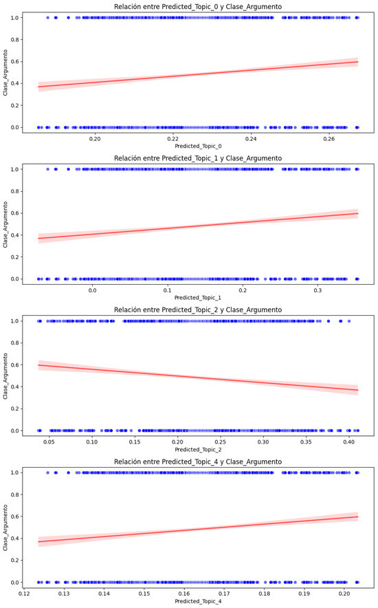 Figure 8. Causal effect relationship between statistically significant Predicted_Topic and Argument_Class.From Figure 8, the following interpretation can be made:The red line helps us visualize the average effect of each Predicted_Topic on the Argument_Class and indicates the type and strength of the relationship. The slope of the line reflects the direction and magnitude of the association between the Predicted_Topic and Argument_Class. The dispersion of the blue points around the red line suggests variability in the data: if the points are close to the line, it implies a stronger relationship, i.e., less variability, while if the points are more dispersed, then the relationship is weaker and there could be other factors affecting the Argument_Class. The red line mainly shows the central tendency of the relationship; for example, a positive slope indicates that as the Predicted_Topic increases, then the Argument_Class also increases, while a negative slope indicates the opposite. The graph shows how this pattern changes concerning Argument_Class when Predicted_Topic varies. For example, we can see that Predicted_Topic_0, Predicted_Topic_1, and Predicted_Topic_4 maintain positive slopes while Predicted_Topic_2 maintains a negative slope, as shown in the graph of Predicted_Topic concerning Argument_Class with a 95% confidence interval (Figure 7), which shows that the model is robust and there is no deviation in its results regarding the estimation of the causal effect.
5.1.2. With Synthetic Data
Analysis and interpretation of the results in Table 13:
Regarding the coefficients of the predictors, each coefficient indicates the expected change in the dependent variable (Argument_Class) associated with a unit change in the corresponding predictor variable, leaving the others constant. Since the Argument_Class variable has two values (0 and 1), the model reflects how the predictor variables influence the result of Argument_Class = 1, maintaining a base or reference (const = 0.4149) when all the predictors are equal to zero (0). In this context, an analysis of each of the topics is presented, as follows:
- Predicted_Topic_0: The increases in this topic are positively related to the probability of the argument_class. It has a positive and highly significant coefficient (p < 0.05). This implies that as the values of these topics increase, the probability of Argument_Class = 1 also increases.
- Predicted_Topic_1: Reflects a negative and weakly significant relationship with Argument_Class. A negative and marginally significant coefficient (p = 0.043) suggests that this topic has a slightly negative relationship with Argument_Class = 1; that is, an increase in this predictor variable decreases the probability of Argument_Class = 1.
- Predicted_Topic_2: Has no significant effect on Argument_Class. This predictor does not contribute in a relevant way to the model’s ability to determine Argument_Class.
- Predicted_Topic_3 and Predicted_Topic_4: Both predictors reflect a positive relationship with Argument_Class. They have positive and very significant coefficients (p < 0.05). This implies that as the values of these topics increase, the probability of Argument_Class = 1 also increases.
- The intercept (const) of 0.4149 (41.49%) represents the probability of the base (Argument_Class = 1) when all predictors are 0. In this case, it is close to 50%, suggesting a relatively balanced result for Argument_Class = 1 versus Argument_Class = 0.
Regarding the robust model, after the experiments were performed with other models (OLS, LR), LSR (Least Squares Regression) was the right choice because it efficiently handles outliers and provides reliable estimates, which is evidenced by the rapid convergence of the model and especially by the significance of the coefficients. Regarding the estimated causal effect, since “date” is the instrumental variable, the coefficient values reflect the adjusted estimate of how the topics through “date” causally affect the variable “Argument_Class”. The most significant or influential predictors are Predicted_Topic_0, Predicted_Topic_3, and Predicted_Topic_4, because they positively impact Argument_Class = 1. Predicted_Topic_1 has a slight negative effect, while Predicted_Topic_2 is not significant. To provide greater transparency to the results obtained in the coefficients of each topic regarding its causal effect on Argument_Class, 95% confidence intervals were included so that the results can be presented graphically, and the results and significance are shown in Figure 9.
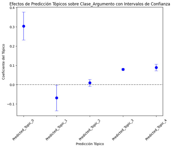
Figure 9.
Causal effect of Predicted_Topic with Argument_Class including 95% confidence intervals.
Given that it was necessary to implement a robust regression model (RLM) in the second regression, the following figure presents the non-linear relationships and allows us to observe more complex patterns (Figure 10). Regarding the pattern or trend, the regression line allows us to estimate the average change in the value of Argument_Class can change when the value of the topic varies. If we have a positive slope, this indicates that as the value of the topic increases, the Argument_Class also increases, while a negative slope indicates the opposite. Regarding the inclination of the red line, the direction and inclination of this line reflect the direction and magnitude of the association between the Predicted_Topic and Argument_Class, which should be reflected in the estimation of the causal effect of Predicted_Topic and Argument_Class. In this regard, Topic_0 and Topic_1 maintain a positive and negative slope, respectively: Predicted_Topic_4 maintains a positive slope in accordance with the estimation of its causal effect. However, Predicted_Topic_3 maintains a negative slope, evidencing an inconsistency in the estimation of its causal effect (Figure 9).
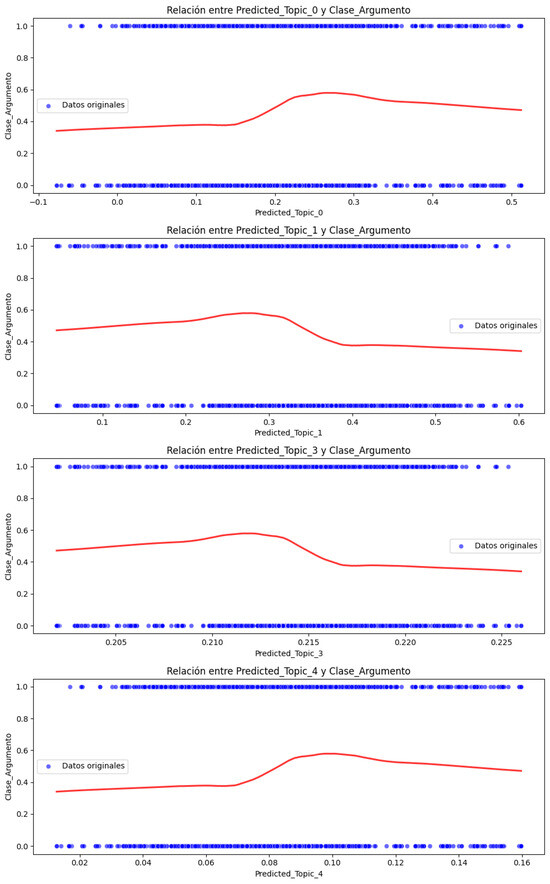
Figure 10.
Causal effect relationship between significant Predicted_Topics and Argument_Class (smoothing curve).
5.1.3. Discrepancies in the Behaviour of the Models Concerning the Estimation of the Causal Effect
Regarding the original data set, the causal effect relationship between statistically significant predicted topics and class demonstrates that the method and model used are robust, and the results do not deviate from the estimation of the overall causal effect.
Regarding the synthetic data set, Predicted_Topic_3 was found to be inconsistent in the estimation of the overall causal effect. To analyze the deviation of the Predicted_Topic_3 from its causal effect estimate for the Argument_Class, simple regression was implemented to eliminate possible influences from other topics and to verify whether the coefficient of Predicted_Topic_3 remained positive. As a result (Table 17), it was verified that Predicted_Topic_3 remained negative, while with LSR, it was positive (Table 13).
Table 17.
Simple regression results for each significant topic.
In Table 17, an equal p-value can be seen for each relevant topic. Correlation analysis was used to analyze the collinearity between the predicted topics to demonstrate how the collinearity and the quality of the data generated by the GPT-35-turbo-0125 model affects the results; see Figure 11.
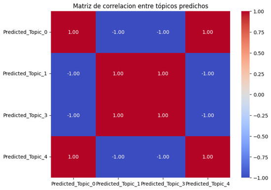
Figure 11.
Correlation matrix between the relevant Predicted_Topics.
Additionally, Figure 12 shows a comparative graph between the OLS and RLM coefficients.
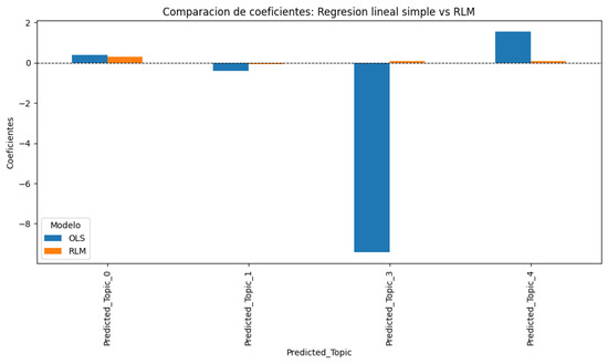
Figure 12.
Comparison of coefficients obtained with the OLS and RLM models.
In Figure 12, we can see that only Predicted_Topic_3, when using RLM, yields a direction opposite to that of an OLS regression. We see how the coefficients of the simple linear regression OLS for an RLM can differ significantly, which shows that the RLM model was the optimal choice because it adjusted the coefficients better, assigning more reasonable values to the topics in the face of collinearity. In this regard, we can see that the OLS regression suffered large deviations, for example, with Predicted_Topic_3, due to the most important aspects, presented as follows:
- Synthetic data quality: The GPT-35-turbo-0125 model generated a significant degree of homogeneity in the generated words (e.g., important, fundamental, some discourse markers, and linking words), which may have reduced the LDA model’s ability to identify better-differentiated topics. This also confirms the current limitations of synthetic data in domain-specific contexts. This relates to the extreme collinearity in the Predicted_Topic, which made interpretation and analysis difficult.
- Impact of collinearity: The coefficient comparison graph of the Simple OLS Regression model and the Robust RLM regression model reinforces LSR was an appropriate choice ffor the final model at the second regression stage, as it successfully addressed these issues.
- Visualization of complexity: The patterns between topics and classes are not linear in the individual scatter plots for each predicted topic, including smoothing curves (Figure 10). This non-linearity may be another source of the discrepancy observed in the Predicted_Topic_3.
5.2. Performance During the Retraining of the Three Best DL Models
The three best DL models were retrained using performance metrics on unseen data. Upon completion of this process, the predicted data sets were generated.
5.2.1. Behavior and Performance of the Best Model
The configuration of the best model architecture (CNN-LSTM-MLP) included the “Cyclical Learning Rate” method. Additionally, a callback was implemented to save the best model during training. The results obtained are as follows.
In Figure 13, (a) shows how the CLR method seeks to take advantage of different learning rates to improve model convergence, demonstrating that the CLR method worked as expected due to the pattern of triangles that was formed, providing a balance between exploration and the model’s ability to generalize. (b) and (c) show the model accuracy and model loss, respectively. Overfitting was generated in the fifth epoch, which was temporary because the training and validation curves converged again. Between epochs 6 and 10, the training and validation show a better balance, probably thanks to the CLR’s dynamic adjustment of the learning_rate. Epochs from approximately 12 to 25 show how the separation stabilizes within a moderate range of epochs, indicating that the model reached a solid equilibrium. With the values shown in (d), a sensitivity of 82.62% and a specificity of 86.49% were obtained, which are balanced values and reflect no evident bias toward the prediction of false positives or false negatives. The precision (86.57%) and high specificity reflect that the model avoids false positives. It also achieved an Accuracy of 84.50% and an F1 score of 84.55%.
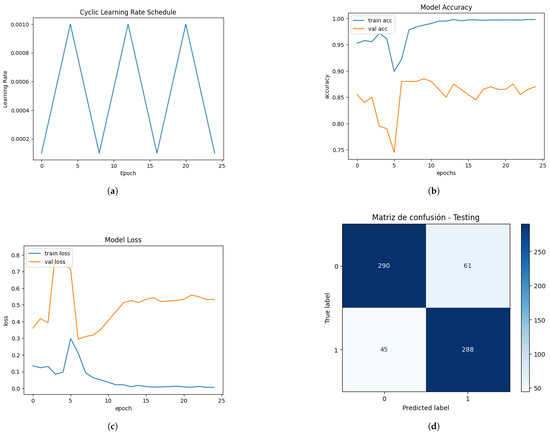
Figure 13.
This is a wide figure. The schemes follow the same formatting. If there are multiple panels, they should be listed as follows: (a) learning rate variation during training; (b) model accuracy—CNN-LSTM-MLP; (c) model loss—CNN-LSTM-MLP; (d) confusion matrix—CNN-LSTM-MLP.
Figure 14 shows the confusion matrix generated by the best CNN-LSTM-MLP model (with automatic saving) obtained during training. This model validates the best value of the val_accuracy metric that the model can achieve during retraining. From the values shown in Figure 14, a sensitivity of 84.05% and a specificity of 87.68% were obtained, which are balanced values and reflect no evident bias toward the prediction of false positives or false negatives. The precision (86.57%) and the high specificity reflect that the model is good at avoiding false positives. Likewise, the improvement in the accuracy (85.82%) and the F1 score (85.88%) of the previous model positions this model as the most balanced and robust.
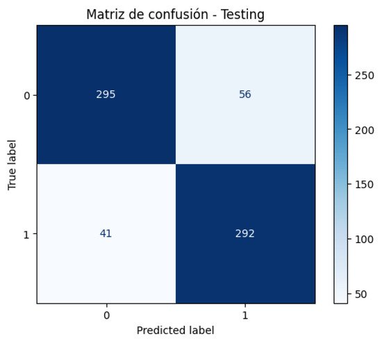
Figure 14.
Confusion Matrix—CNN-LSTM-MLP Best Model.
5.2.2. Comparison of Performance Metrics of the Top Three Models
The comparison of relative performance metrics during model training is presented in Figure 15. The best model of the hybrid CNN-LSTM-MLP architecture achieved a validation accuracy of 88.50% (val_accuracy) and a validation loss of 0.3534 (val_loss) at epoch 10 using a learning rate of 3.25 × 10⁻⁴. The best three models and their weights were saved (.keras format and .weights.h5 format, respectively). Likewise, in the case of the best model, the model with the best performance during training was saved for possible future evaluations (’best_cnn_lst_mlp_cyclicLR.keras’). Regarding the CNN model, epoch 9 was selected because it presented the lowest validation loss value (val_loss) of 0.3047, compared to the val_loss of 0.3349 observed in epoch 13. Both epochs showed the same val_accuracy of 0.8600, so the loss-based metric was used to make the choice. In the case of the CNN-LSTM model, the values were taken from the last training epoch (epoch 10) using the early stopping criterion, and for the CNN-LSTM-MLP model, the values from epoch 10 were selected, which was where the model achieved the highest accuracy (Table 18).
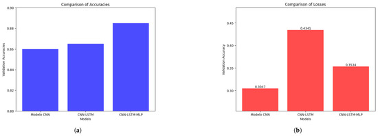
Figure 15.
Step 3 has two phases: (a) comparison of accuracies during training; (b) comparison of losses during training.
Table 18.
Summary of Val_Accuracy and Val_Loss metrics.
Finally, Table 19 emphasizes that the main criterion for selecting the best three models was the value obtained in the “test_accuracy” because it reflects the performance of the DL models with data not used during the training or retraining stages.
Table 19.
Top three DL models’ performance on unseen data.
5.3. Comparison of Global Causal Effects with Causal Effects of Predicted Subsets
The results in this section reveal interesting findings regarding the following question: Are the AI models that achieve the best accuracy percentages the best models? In this regard, the results found for the best model and the third-best model are presented (the second-best model yielded very similar results to the best model).
5.3.1. The Best Model
Analysis and interpretation of results of the best DL model (Table 14):
- The coefficients show the estimated impact of each topic (instrument) on the dependent variable (Class_Argument). Each positive coefficient reflects a direct relationship, while a negative one reflects an inverse relationship. Predicted_Topic_0_Proportion, Predicted_Topic_1_Proportion, and Predicted_Topic_4_Proportion have values less than 0.05, indicating that their effects on Class_Argument are significant. However, Predicted_Topic_2_Proportion and Predicted_Topic_3_Proportion are not statistically significant (p-values of 0.062 and 0.152, respectively), which indicates that these particular topics might not have a relevant effect on the dependent variable.
- Regarding the sign and magnitude of the coefficients, Predicted_Topic_0_Proportion, Predicted_Topic_1_Proportion, and Predicted_Topic_4_Proportion have positive coefficients, suggesting a direct association with Argument_Class. Predicted_Topic_2_Proportion and Predicted_Topic_3_Proportion have negative coefficients and are significant, indicating an inverse association with Argument_Class.
- Regarding the interpretation of the causal effect, these coefficients indicate that there is a significant relationship between certain topics, such as Predicted_Topic_0, Predicted_Topic_1, and Predicted_Topic_4 with Argument_Class, to the extent that changes in the Predicted_Topics affect the Argument_Class.
To clarify the results obtained on the coefficients of each topic regarding its causal effect on the Argument_Class, 95% confidence intervals were included so the results could be presented graphically, and the results and their significance could be fully understood (a) (Figure 16). To complete the analysis and interpretation of the causal effect results, individual scatter plots were used for each significant topic (Predicted_Topic_0, Predicted_Topic_1, and Predicted_Topic_4) to the Argument_Class. Likewise, the regression line was added to show the trend of each Predicted_Topic_Proportion concerning the Argument_Class (Figure 16b). The red line shows the average effect of each Predicted_Topic_Proportion on the Argument_Class and indicates the type and strength of the relationship. The slope of the line reflects the direction and magnitude of the association between Predicted_Topic_Proportion and Argument_Class. It mainly shows the central tendency of the relationship; in this case, the positive slope indicates that as the value of Predicted_Topic_Proportion increases, then Argument_Class also increases. We can see in the graph that Predicted_Topic_0, Predicted_Topic_1, and Predicted_Topic_4 maintain positive slopes, as demonstrated in the graph of Predicted_Topic_Proportion against Argument_Class, with a 95% confidence interval (a), thus proving that the model is robust. However, it is verified that the behavior pattern of the predicted topics generated by the best DL model deviates from the global causal effect estimated for the original data set because Predicted_Topic_2 is not statistically significant. It should be noted that the second-best model showed the same behavior (Table 15).

Figure 16.
Effects of the prediction of topic proportions on Argument_Class—best model: (a) topic proportion prediction with confidence intervals; (b) causal effect relationship between proportion of statistically significant topics and Argument_Class.
5.3.2. The Third-Best Model
Analysis and interpretation ofthe results of the best DL model (Table 16):
- Coefficients: Predicted_Topic_0_Proportion, Predicted_Topic_1_Proportion, Predicted_Topic_2_Proportion, and Predicted_Topic_4_Proportion have values less than 0.05, which indicates that their effects on Argument_Class are significant. However, Predicted_Topic_3_Proportion was not statistically significant (p-value of 0.113), indicating that this particular topic might not have a relevant effect on the dependent variable.
- Regarding the sign and magnitude of coefficients, Predicted_Topic_0_Proportion, Predicted_Topic_1_Proportion, and Predicted_Topic_4_Proportion have positive coefficients, suggesting a direct relationship with Argument_Class, while Predicted_Topic_2_Proportion has a negative coefficient, reflecting an inverse relationship with Argument_Class. This indicates that an increase or decrease in these topics predicts an increase or decrease in the probability of the topic belonging to a specific Argument_Class class.
- Regarding the interpretation of the causal effect, these coefficients indicate that there is a significant relationship in topics such as Predicted_Topic_0_Proportion, Predicted_Topic_1_Proportion, Predicted_Topic_2_Proportion, Predicted_Topic_4_Proportion with Argument_Class, to the extent that changes in these Predicted_Topics_Proportion affect Argument_Class.
To clarify the results obtained regarding the coefficients of each topic and its causal effect on the Argument_Class, 95% confidence intervals were included so that the results could be presented graphically and the significance could be obtained, as shown in Figure 17a:
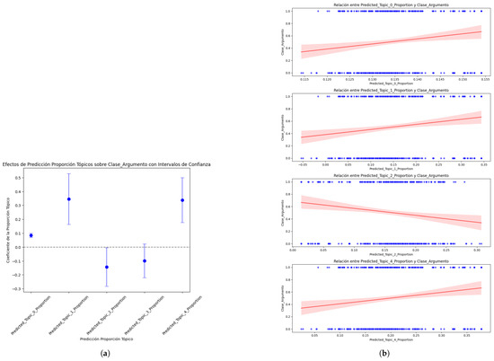
Figure 17.
Effects of the prediction of topic proportions on Argument_Class—third-best model: (a) topic proportion prediction with confidence intervals; (b) causal effect relationship between proportion of statistically significant topics and Argument_Class.
In Figure 17b, a scatter graph was included for each significant topic to visualize the pattern that “Predicted_Topic_topic_Proportion” follows for “Argument_Class”. The red line mainly shows the central tendency of the relationship; for example, a positive slope indicates that as Predicted_Topic_Proportion increases, then Argument_Class also increases, while a negative slope indicates the opposite. We see in the graph that Predicted_Topic_0_Proportion, Predicted_Topic_1_Proportion, and Predicted_Topic_4_Proportion maintain positive slopes while Predicted_Topic_2_Proportion presents a negative slope as demonstrated in the graph of Predicted_Topic_Proportion against Argument_Class with a 95% confidence interval, thus proving that the model is robust. Finally, it is shown that the third-best DL model aligns with the results obtained after estimating the overall causal effect on the original data set, not only because Predicted_Topic_2 is statistically significant but also because the model manages to capture its inverse trend (negative slope), unlike Predicted_Topic_0, Predicted_Topic_1, and Predicted_Topic_4 (see (Figure 8)). These findings demonstrate that the best DL model (based on predictive performance) does not necessarily align with the estimated overall causal effect relationship.
6. Discussion
6.1. From the Perspective of Causal Inference and Estimation
In line with [38], we consider that the findings of our research are aligned with the third perspective, “Causality for XAI”, because the implementation of causal inference techniques in AI models constitutes the preparatory stage of consolidating XAI (eXplainable Artificial Intelligence) by naturally facilitating its interpretation. On the other hand, it is important to mention that causal inference reveals whether there is a cause–effect relationship between certain characteristics and the prediction, while causal estimation quantifies this relationship through the model’s results. In our research, these two perspectives were implemented to demonstrate the robustness of the models and statistical methods used to apply the proposed IV-NLP method. Upon investigation, the causal inference methods were found to have followed two important approaches.
The first approach prioritizes performance metrics when predicting the causal effect by minimizing the MSE (Mean Square Error) metric. The second approach prioritizes the explainability of causal effects by facilitating their interpretability. In the first approach, the work of [39] addressed the problem of nonlinearity between variables Y and X. It proposed Kernel Instrumental Variable (KIV) as a nonparametric IV method prioritizing predictive performance. However, it did not explicitly address the challenges of causal inference in NLP. The work of [40] proposed using the Deep Feature Instrumental Variable Regression (DFIV) method to learn the optimal representations of instrumental and treatment variables. While DFIV outperformed the estimation accuracy achieved by KIV, its applicability depends on the availability of sufficiently large, structured, or numerical data, making it less applicable to NLP tasks. Likewise, ref. [41] proposed the Deep IV method to optimize the accuracy in estimating causal effects by using neural networks in nonlinear relationships between instrumental variables and treatments. In our research, the problem of nonlinearity between variables Y and X arose due to the presence of atypical elements, homogeneity, and heteroscedasticity in the synthetic data (GPT-3.5-turob-0125), so, at the second stage of the instrumental analysis, the Robust Regression Model (RLM) with the Huber norm was applied to mitigate this problem.
In the second approach, ref. [42] proposed using Causal Shapley Values (CSV) as a tool to improve the causal interpretability of deep learning models by implementing Pearl, Judea’s concept [20] regarding the causal structure of the data. Along these same lines, Instrumental Variables-based Regression Methods offer interpretability in estimations of the causal effect. Using this framework, IV-NLP has two stages: the first stage performs causal inference and estimation by integrating IV-based methods and statistical methods such as logistic regression and robust regression to mitigate the presence of non-linear relationships, heteroscedasticity, and outliers (original data and synthetic data); in the second stage, it is possible to capture causal patterns in the predicted data using the best DL models in NLP. When this proposal was applied to the field of NLP, it was possible to explain and interpret the results using a causal approach, but at the cost of certain limitations in the flexibility of the models.
Finally, ref. [43] proposed a more balanced approach with the Causal Forests method, which allows for the heterogeneity of the treatment effects in different population groups to be understood while maintaining a balance with the precision needed to estimate the causal effect. With IV-NLP, not only is the precision measured in terms of the stability and statistical significance of the coefficients obtained in the second stage of the instrumental analysis, an understanding can be obtained of the causal patterns underlying the data to interpret DL models in the field of NLP. This justifies the choice of the models and techniques, where the IV-NLP method was applied to balance these two approaches.
6.2. From the Perspective of the Characteristics of the Data Set
Yao et al. [16] present a compilation of data sets commonly used in causal inference, highlighting the importance of structured attributes regarding treatments, covariates, and outcomes. However, it was shown that the absence of explicit treatments does not prevent the implementation of causal inference methods if an underlying structure allows for the identification of the causal effect [23]. Our research used a data set with 4015 records and a synthetic data set with 3966 records with low dimensionality. Although our research worked with a data set with a reduced number of features, the presence of endogeneity and the knowledge of the domain motivated the application of the IV method. This data set does not define an explicit treatment; however, this approach allowed us to estimate the causal effect of the explanatory variable on the target variable by reducing the bias introduced by unobserved confounding elements. This perspective broadens the understanding of the applicability of IV in the field of NLP, where the conventional data structure for causal inference is not necessarily directly observable.
6.3. From the Perspective of Synthetic Data Generation and Causal Inference Techniques
Wood-Doughty et al. [44] proposed a framework based on LDA and GPT-2 to produce high-dimensional synthetic textual data with causal effects controlled by propensity score matching and inverse propensity weighting (IPW) methods. However, these methods may fail to adjust the causal effect due to unobserved confounders in the textual data. In contrast, we applied IV-NLP with a low-dimensional data set, which facilitated the use of the LDA model to segment predefined topics from the original data and applied the IV method to estimate the causal effects to identify whether the causal pattern of the synthetic data aligned with the causal pattern of the original data. The authors of [45] used the GPT-3 model (“text-davinci-003”) to address the class imbalance problem in sentiment analyses. Their study showed that using synthetic data improved sentiment classification. However, the presence of redundant synthetic data affected the diversity of their data. Along these lines, in our study, when applying IV-NLP, the GPT-3.5-turbo-0125 model was first used with a variation of the standard RAG technique to increase the amount of data in the original data set and mitigate false synthetics; however, after conducting a causal analysis on the synthetic data, it was decided not to use them for prediction tasks because their causal pattern deviated from the causal pattern in the original data due to their homogeneity and collinearity, which impacted the diversity of the data set.
7. Conclusions and Future Work
Causality and explanation are complementary concepts in artificial intelligence, so they must be treated together. Causality naturally gives way to explainability, allowing for robust and explainable models to be developed. The application of the proposed method, IV-NLP, demonstrates that a methodological choice based on a causal approach may not only depend on increasing the predictive capacity of the model but also on the need to more clearly understand the dynamics of the treatment of the outcome variable, ensuring that the causal pattern identified in the observed data is consistent with the behavior of the predicted data. This perspective is important because, in the field of NLP, the need for high accuracy in causal estimation is less critical, and interpretation plays a more dominant role. The IV method constitutes an alternative route to implementing causal inference and estimation techniques in NLP, specifically in data structures where one or more treatments do not necessarily explicitly exist. Likewise, the IV method applies to data sets with low dimensionality, favoring the robustness of the models in small data sets. Besides these, the selection of the best AI (ML, DL) model should not be based solely on performance metrics on unseen data. Rather, the causal pattern in the predicted data should be considered so that the selected AI model aligns with the data’s overall causal effect pattern. On the other hand, the intervention method used to generate synthetic textual data (Figure 2) emphasized the need to correctly generate argumentative and non-argumentative texts; however, GPT-3.5-turbo-0125 did not always adequately modify the original text. These findings reveal a critical need to evaluate the quality of synthetic data before incorporating them into specific knowledge domains. We believe that mitigating this problem requires a more in-depth analysis of the reliability of generative models as substitutes for real data in specific domains. This work serves as a wake-up call to assess the feasibility of using synthetic data in real-world applications, which has significant implications for causal inference, especially in sensitive or highly structured domains.
In future work, from the perspective of causal inference and estimation, the Causal Forests model [43] and the CSV tool [42] could be included in order to compare their results regarding the variations in treatment impact in different scenarios to facilitate the understanding of causal patterns in NLP and mitigate the limitations found in the flexibility of traditional models. From the perspective of data structure, working with high-dimensional data sets that include the presence of confounders in the field of NLP will allow for the use of other more sophisticated IV regression methods during the application of the IV-NLP method. From the perspective of synthetic data generation, improving the quality and validation of the data generated by an LLM can be mitigated using GPT-4, GPT-4o, and GPT-4-turbo. To improve the proposed IV-NLP methodology, IV-NLP should be applied to other NLP tasks, such as implementing ML models in other two-class and multi-class problems. IV-NLP should also be applied to other data sets based on texts written in native English and with much larger data sets. Finally, it is recommended that when applying the IV-NLP method to other domains, the predicted data sets are generated during the training stage. This will avoid additional effort in retraining the models. Additionally, the results produced by a superior GPT model should be verified to assess the extent to which homogeneity is reduced and the diversity of the outputs is increased. If the causal effect pattern of the synthetic data aligns with the real data, then the synthetic data could be used in predictive tasks.
Author Contributions
Conceptualization, J.M.F.-L. and F.J.R.-P.; methodology, Y.G.-M.; software, Y.G.-M.; validation, Y.G.-M.; formal analysis, Y.G.-M.; investigation, Y.G.-M.; resources, Y.G.-M.; data curation, Y.G.-M.; writing—original draft preparation, Y.G.-M.; writing—review and editing, Y.G.-M.; visualization, Y.G.-M.; supervision, J.M.F.-L. and F.J.R.-P.; project administration, J.M.F.-L. and F.J.R.-P.; funding acquisition, Y.G.-M. All authors have read and agreed to the published version of the manuscript.
Funding
This research received no external funding.
Institutional Review Board Statement
Not applicable.
Informed Consent Statement
Not applicable.
Data Availability Statement
The data sets IV-NLP associated with this study is publicly available in Mendeley Data. The data set DOI is 10.17632/rcn3swj868.2.
Conflicts of Interest
The authors declare no conflicts of interest.
Appendix A. Recovering Features from Original and Synthetic Data Sets
- Step 1: Recovering ‘Date’ and ‘Id’ features to the original datasets (Figure A1)The data set format was converted (from ‘utf-8’ to ‘latin-1’) with the attributes Id, Text, and Class_Argument. The attribute ‘Date’ was retrieved from the annotated data set. The Pandas merge library was used and 2895 records were obtained, with the ‘Date’ characteristic being retrieved automatically. The assignment of the ‘Date’ and the ‘ID’ of the rest of the records was carried out manually. The manual verification of the records was necessary because the IDs were compared with their respective texts, so a significant effort was made in terms of time by the annotators to guarantee the quality of the data.
- Step 2: Feature recovery on the six (06) original datasets distributed from the global corpus (Figure A2)An automated procedure was implemented using the Pandas (version 2.1.4) libraries with the Keras (version 3.4.1) framework to filter the global data set generated in Step 1. Duplicate records were eliminated, and subsequently, the verification of each feature recovery process was carried out for each of the six (06) data sets, finding only one record from the set of argumentative texts of the training set in which the match could not be established because it was not located in the global data set of Step 1; this was eliminated, leaving the set of argumentative texts of the “Training” set with 1526 records with their attributes duly recovered. No incidence was found in the rest of the data sets, and the attributes of the six (06) data sets were successfully recovered (see Figure A3).
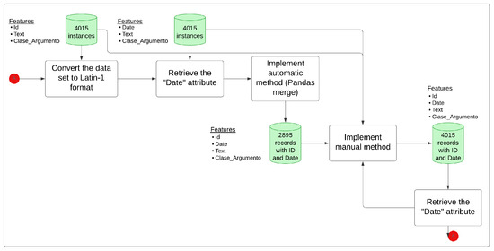
Figure A1.
Process of recovering the features ’Id’ and ’Date’ to the original global data set.
Figure A1.
Process of recovering the features ’Id’ and ’Date’ to the original global data set.
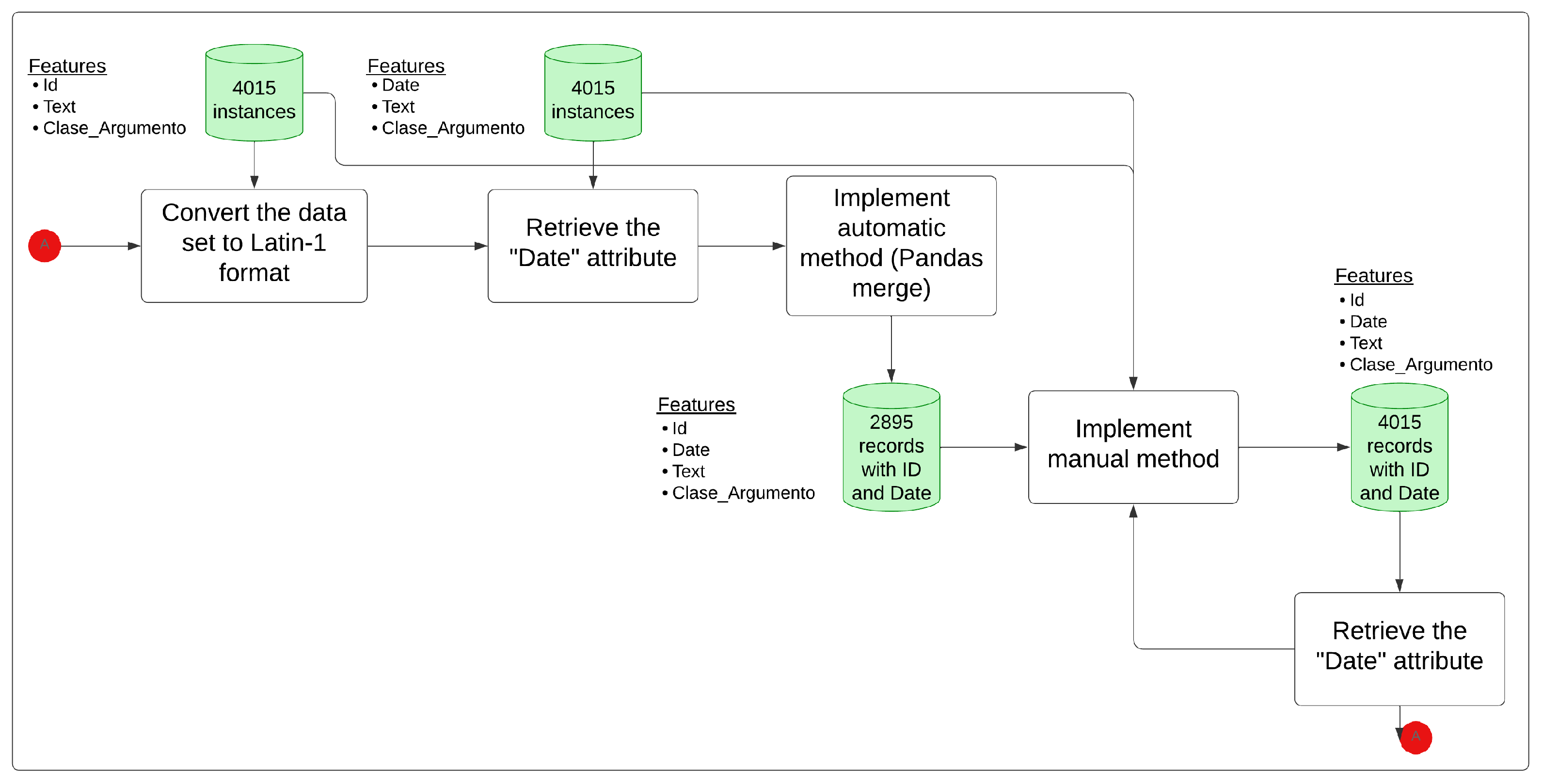
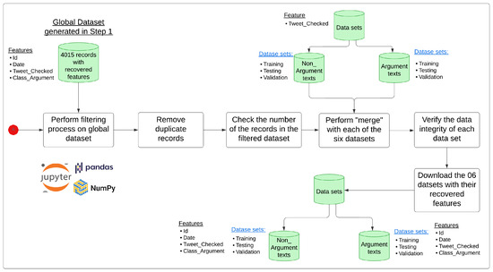
Figure A2.
Feature retrieval in the six datasets with original texts.
Figure A2.
Feature retrieval in the six datasets with original texts.
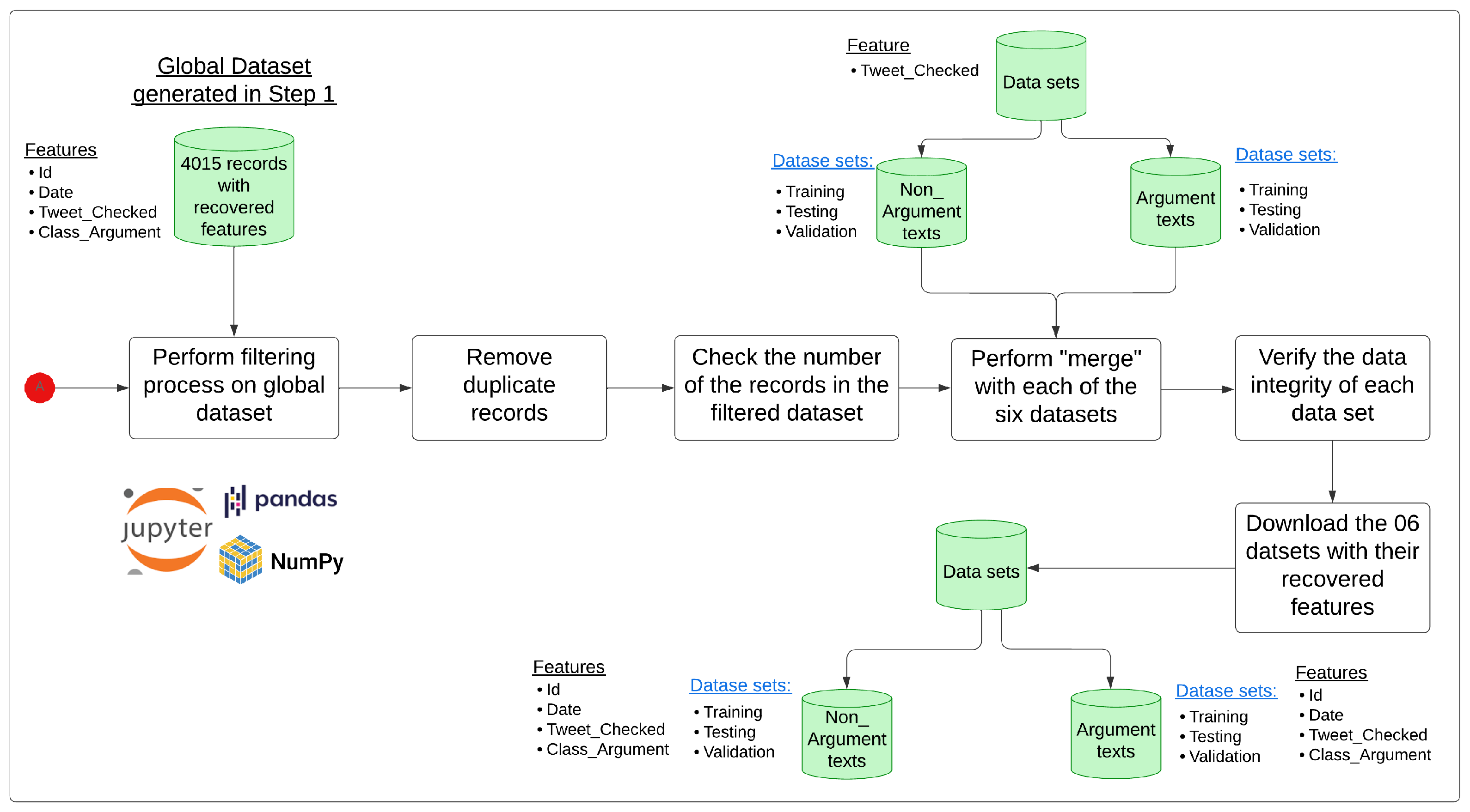
- Step 3: Feature recovery on the six (06) datasets with synthetic texts generated by the GPT-3.5-turbo-0125 modelThis step was carried out in two (02) phases:
- –
- Phase 1: Assignment of ‘Date’ and ‘Id’ to the six (06) sets of synthetic texts generated by the GPT35-turbo-0125 model (OUTPUT of the Intervention Method defined in Figure 2). Figure A3 graphically shows the procedure carried out in this phase.The process consisted of adding the columns ‘Date’ and ‘Id’ according to the index position of the Excel file of the data set, ensuring that there was the same number of records in both data sets. This was because code routines were implemented so that the GPT3.5-turbo-0125 model would generate an alternative text for each text in the data set (See Figure 2). During the process of assigning the attributes ‘Date’ and ‘Id’ to the data sets with generated texts, only one incident was found, so two records were eliminated from the set of argumentative texts in the training set because the GPT3.5-turbo-0125 model generated two different textual records for the same record for these two records. In the remaining five (05) sets of generated texts, there was no incidence because the model generated, in all cases, only one alternative text in front of each of the records of the original sets of texts. Table 4 shows the results obtained. The data sets for the generated texts had the following structure: Date, Original_Id, Tweet_Checked, Clase_Argumento (where Original_Id is the Id value of the data sets with original texts, which will be helpful in terms of data traceability during the data interpretation stage).
- –
- Phase 2: Assignment of ‘Date’ and ‘Id’ to the six (06) sets of synthetic texts generated by the GPT35-turbo-0125 model (validation of texts generated by the model defined in the intervention method described in Figure 2). Figure A3 graphically shows the procedure carried out in this phase.Records whose generated texts were the same as those of the texts generated once they passed through data validation at the end of the intervention method were filtered out. This process was repeated for each pair of data sets (training, testing, and validation). For the training set, the attributes ‘Date’ and ‘Id’ were automatically recovered for 1500 and 1537 records in the set of argumentative and non-argumentative texts, respectively. A manual verification of the sets of argumentative and non-argumentative texts was then performed to complete the attributes ‘Date’ and ‘Id’ in the 25 and 27 missing records, respectively, to correctly assign these two attributes in line with the intervention method detailed in Figure 2. The procedure performed for the training set was replicated for the test and validation sets. Likewise, no incidents were presented.
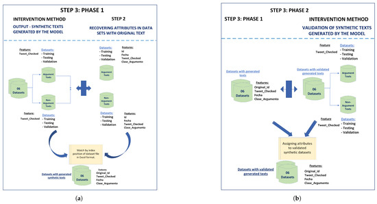
Figure A3.
Step 3 has two phases: (a) Step 3—Phase 1: the assignment of features in the synthetic text sets generated by the model; (b) Step 3—Phase 2: the assignment of features in the generated and validated text sets.
Figure A3.
Step 3 has two phases: (a) Step 3—Phase 1: the assignment of features in the synthetic text sets generated by the model; (b) Step 3—Phase 2: the assignment of features in the generated and validated text sets.
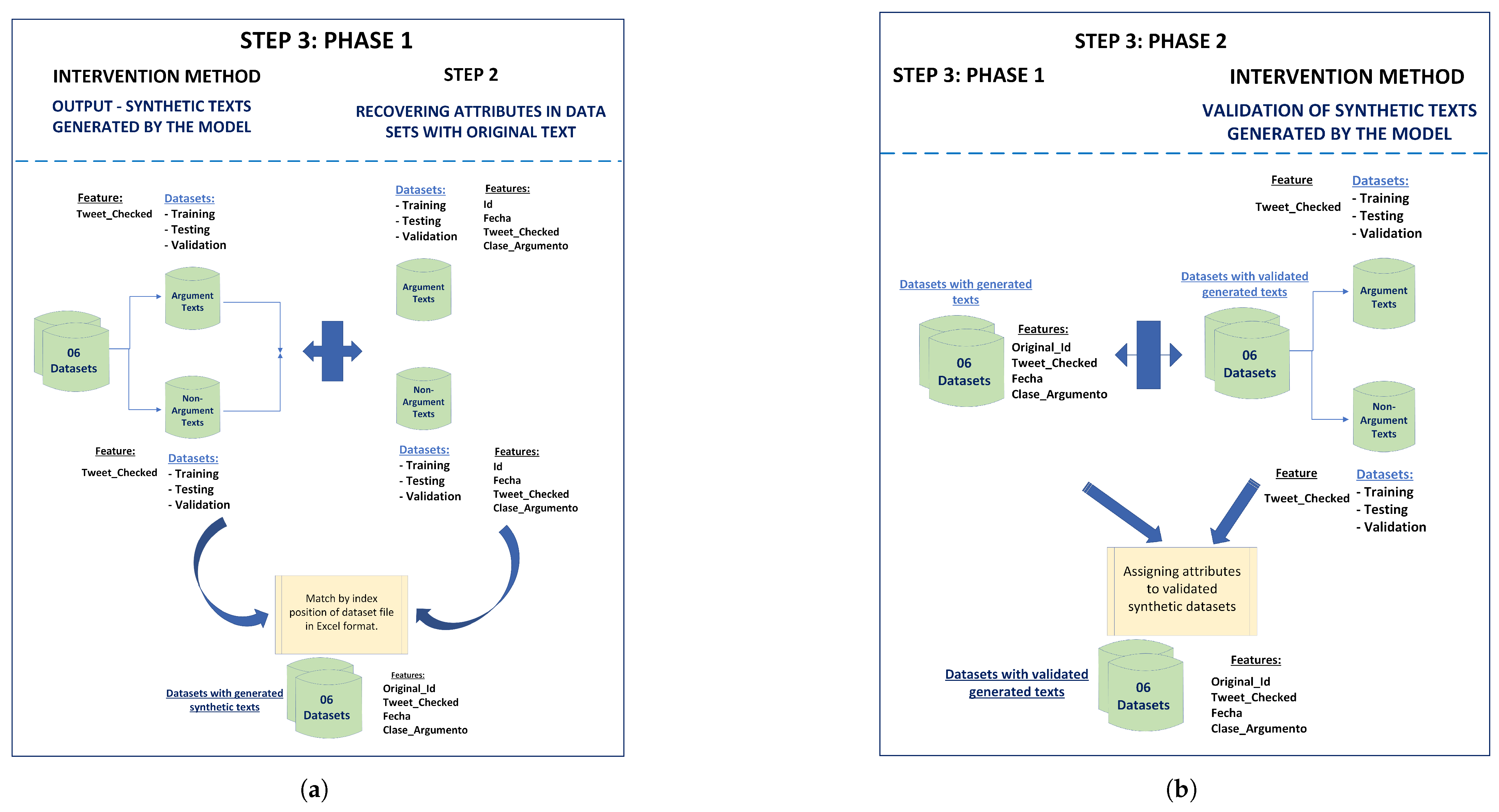
References
- Ludwig, J.; Mullainathan, S. Machine Learning as a Tool for Hypothesis Generation. Q. J. Econ. 2024, 139, 751–827. [Google Scholar] [CrossRef]
- Scholkopf, B.; Locatello, F.; Bauer, S.; Ke, N.R.; Kalchbrenner, N.; Goyal, A.; Bengio, Y. Toward Causal Representation Learning. Proc. IEEE 2021, 109, 612–634. [Google Scholar] [CrossRef]
- Spirtes, P. Introduction to causal inference. J. Mach. Learn. Res. 2010, 11, 1643–1662. [Google Scholar]
- Yang, J.; Han, S.C.; Poon, J. A survey on extraction of causal relations from natural language text. Knowl. Inf. Syst. 2022, 64, 1161–1186. [Google Scholar] [CrossRef]
- Feder, A.; Oved, N.; Shalit, U.; Reichart, R. CausaLM: Causal Model Explanation Through Counterfactual Language Models. Comput. Linguist. 2021, 47, 333–386. [Google Scholar] [CrossRef]
- Jiao, L.; Wang, Y.; Liu, X.; Li, L.; Liu, F.; Ma, W.; Guo, Y.; Chen, P.; Yang, S.; Hou, B. Causal Inference Meets Deep Learning: A Comprehensive Survey. Research 2024, 7, 467. [Google Scholar] [CrossRef]
- Chen, Y.; Bühlmann, P. Domain adaptation under structural causal models. J. Mach. Learn. Res. 2021, 22, 1–80. [Google Scholar]
- Bound, J.; Jaeger, D.A.; Baker, R.M. Problems with instrumental variables estimation when the correlation between the instruments and the endogenous explanatory variable is weak. J. Am. Stat. Assoc. 1995, 90, 443–450. [Google Scholar] [CrossRef]
- Angrist, J.; Imbens, G. Identification and Estimation of Local Average Treatment Effects. 1995. Available online: https://www.nber.org/papers/t0118 (accessed on 10 March 2025).
- Molak, A.; Jaokar, A. Causal Inference and Discovery in Python: Unlock the Secrets of Modern Causal Machine Learning with DoWhy, EconML, PyTorch and More; Packt Publishing Ltd.: Birmingham, UK, 2023; p. 429. [Google Scholar]
- Lu, Y.; Shen, M.; Wang, H.; Wang, X.; van Rechem, C.; Fu, T.; Wei, W. Machine Learning for Synthetic Data Generation: A Review. arXiv 2024, arXiv:2302.04062. [Google Scholar]
- Lewis, P.; Perez, E.; Piktus, A.; Petroni, F.; Karpukhin, V.; Goyal, N.; Küttler, H.; Lewis, M.; Yih, W.t.; Rocktäschel, T.; et al. Retrieval-augmented generation for knowledge-intensive nlp tasks. Adv. Neural Inf. Process. Syst. 2020, 33, 9459–9474. [Google Scholar]
- Hicks, M.T.; Humphries, J.; Slater, J. ChatGPT is bullshit. Ethics Inf. Technol. 2024, 26, 38. [Google Scholar] [CrossRef]
- OpenAI; Achiam, J.; Adler, S.; Agarwal, S.; Ahmad, L.; Akkaya, I.; Aleman, F.L.; Almeida, D.; Altenschmidt, J.; Altman, S.; et al. GPT-4 Technical Report. arXiv 2024, arXiv:2303.08774. [Google Scholar]
- Wu, A.; Kuang, K.; Xiong, R.; Wu, F. Instrumental Variables in Causal Inference and Machine Learning: A Survey. arXiv 2022, arXiv:2212.05778. [Google Scholar]
- Yao, L.; Chu, Z.; Li, S.; Li, Y.; Gao, J.; Zhang, A. A Survey on Causal Inference. ACM Trans. Knowl. Discov. Data 2021, 15, 1–46. [Google Scholar] [CrossRef]
- Sui, Y.; Wang, X.; Wu, J.; Lin, M.; He, X.; Chua, T.S. Causal Attention for Interpretable and Generalizable Graph Classification. In Proceedings of the 28th ACM SIGKDD International Conference on Knowledge Discovery and Data Mining. Association for Computing Machinery, Washington, DC, USA, 14–18 August 2022; pp. 1696–1705. [Google Scholar] [CrossRef]
- Sun, Y.; Kong, L.; Chen, G.; Li, L.; Luo, G.; Li, Z.; Zhang, Y.; Zheng, Y.; Yang, M.; Stojanov, P.; et al. Causal Representation Learning from Multimodal Biological Observations. arXiv 2024, arXiv:2411.06518. [Google Scholar]
- Liu, F. Data Science Methods for Real-World Evidence Generation in Real-World Data. Annu. Rev. Biomed. Data Sci. 2024, 7, 29. [Google Scholar] [CrossRef]
- Pearl, J. Causality: Models, Reasoning, and Inference; Cambridge University Press: Cambridge, UK, 2009. [Google Scholar]
- Angrist, J.D.; Krueger, A.B. Instrumental Variables and the Search for Identification: From Supply and Demand to Natural Experiments. J. Econ. Perspect. 2001, 15, 69–85. [Google Scholar] [CrossRef]
- Martens, E.P.; Pestman, W.R.; de Boer, A.; Belitser, S.V.; Klungel, O.H. Instrumental variables: Application and limitations. Epidemiology 2006, 17, 260–267. [Google Scholar] [CrossRef]
- Angrist, J.D.; Pischke, J.S. Mostly Harmless Econometrics: An Empiricist’s Companion; Princeton University Press: Princeton, NJ, USA, 2009. [Google Scholar]
- Imbens, G.W.; Rubin, D.B. Causal Inference in Statistics, Social, and Biomedical Sciences; Cambridge University Press: Cambridge, UK, 2015. [Google Scholar]
- Stock, J.H.; Watson, M.W. Introduction to Econometrics; Pearson: London, UK, 2020. [Google Scholar]
- Wu, K.; Wang, Z.; Zhao, J.; Xu, H.; Hao, T.; Lin, W. Instrumental variables matter: Towards causal inference using deep learning. In Proceedings of the Journal of Physics: Conference Series; IOP Publishing: Oxford, UK, 2023; Volume 2580, p. 012044. [Google Scholar]
- He, X.; Nassar, I.; Kiros, J.; Haffari, G.; Norouzi, M. Generate, Annotate, and Learn: NLP with Synthetic Text. Trans. Assoc. Comput. Linguist. 2022, 10, 826–842. [Google Scholar] [CrossRef]
- Yang, Y.; Malaviya, C.; Fernandez, J.; Swayamdipta, S.; Le Bras, R.; Wang, J.P.; Bhagavatula, C.; Choi, Y.; Downey, D. Generative Data Augmentation for Commonsense Reasoning. In Proceedings of the Findings of the Association for Computational Linguistics: EMNLP 2020; Cohn, T., He, Y., Liu, Y., Eds.; Association for Computational Linguistics: Stroudsburg, PA, USA, 2020; pp. 1008–1025. [Google Scholar] [CrossRef]
- Li, Z.; Zhu, H.; Lu, Z.; Yin, M. Synthetic Data Generation with Large Language Models for Text Classification: Potential and Limitations. In Proceedings of the Empirical Methods in Natural Language Processing: EMNLP 2023, Singapore, 6–10 December 2023; pp. 10443–10461. [Google Scholar] [CrossRef]
- AlKhamissi, B.; Li, M.; Celikyilmaz, A.; Diab, M.; Ghazvininejad, M. A Review on Language Models as Knowledge Bases. arXiv 2022, arXiv:2204.06031. [Google Scholar]
- Gekhman, Z.; Yona, G.; Aharoni, R.; Eyal, M.; Feder, A.; Reichart, R.; Herzig, J. Does Fine-Tuning LLMs on New Knowledge Encourage Hallucinations? In Proceedings of the 2024 Conference on Empirical Methods in Natural Language Processing (EMNLP). Association for Computational Linguistics, Miami, FL, USA, 12–16 November 2024; pp. 7765–7784. [Google Scholar]
- Feder, A.; Keith, K.A.; Manzoor, E.; Pryzant, R.; Sridhar, D.; Wood-Doughty, Z.; Eisenstein, J.; Grimmer, J.; Reichart, R.; Roberts, M.E.; et al. Causal Inference in Natural Language Processing: Estimation, Prediction, Interpretation and Beyond. Trans. Assoc. Comput. Linguist. 2022, 10, 1138–1158. [Google Scholar] [CrossRef]
- Zhou, L.; Schellaert, W.; Martínez-Plumed, F.; Moros-Daval, Y.; Ferri, C.; Hernández-Orallo, J. Larger and more instructable language models become less reliable. Nature 2024, 634, 61–68. [Google Scholar] [CrossRef] [PubMed]
- Guzmán-Monteza, Y. Assessment of an annotation method for the detection of Spanish argumentative, non-argumentative, and their components. Telemat. Inform. Rep. 2023, 11, 100068. [Google Scholar] [CrossRef]
- Guzman, Y.; Tavara, A.; Zevallos, R.; Vega, H. Implementation of a Bilingual Participative Argumentation Web Platform for collection of Spanish Text and Quechua Speech. In Proceedings of the 3rd International Conference on Electrical, Communication and Computer Engineering, ICECCE 2021, Kuala Lumpur, Malaysia, 12–13 June 2021. [Google Scholar] [CrossRef]
- Saxena, C.; Garg, M.; Ansari, G. Explainable Causal Analysis of Mental Health on Social Media Data. In Proceedings of the Neural Information Processing, Indore, India, 22–26 November 2023; pp. 172–183. [Google Scholar]
- Huber, P.J. Robust estimation of a location parameter. In Breakthroughs in Statistics: Methodology and Distribution; Springer: Berlin/Heidelberg, Germany, 1992; pp. 492–518. [Google Scholar]
- Carloni, G.; Berti, A.; Colantonio, S. The role of causality in explainable artificial intelligence. arXiv 2023, arXiv:2309.09901. [Google Scholar]
- Singh, R.; Sahani, M.; Gretton, A. Kernel instrumental variable regression. Adv. Neural Inf. Process. Syst. 2019, 32, 4595–4607. [Google Scholar]
- Xu, L.; Chen, Y.; Srinivasan, S.; de Freitas, N.; Doucet, A.; Gretton, A. Learning deep features in instrumental variable regression. arXiv 2023, arXiv:2010.07154. [Google Scholar]
- Hartford, J.; Lewis, G.; Leyton-Brown, K.; Taddy, M. Deep IV: A Flexible Approach for Counterfactual Prediction. In Proceedings of the 34th International Conference on Machine Learning, Sydney, Australia, 6–11 August 2017; Precup, D., Teh, Y.W., Eds.; Volume 70, pp. 1414–1423. [Google Scholar]
- Heskes, T.; Sijben, E.; Bucur, I.G.; Claassen, T. Causal shapley values: Exploiting causal knowledge to explain individual predictions of complex models. Adv. Neural Inf. Process. Syst. 2020, 33, 4778–4789. [Google Scholar]
- Wager, S.; Athey, S. Estimation and inference of heterogeneous treatment effects using random forests. J. Am. Stat. Assoc. 2018, 113, 1228–1242. [Google Scholar] [CrossRef]
- Wood-Doughty, Z.; Shpitser, I.; Dredze, M. Generating synthetic text data to evaluate causal inference methods. arXiv 2021, arXiv:2102.05638. [Google Scholar]
- Suhaeni, C.; Yong, H.S. Enhancing Imbalanced Sentiment Analysis: A GPT-3-Based Sentence-by-Sentence Generation Approach. Appl. Sci. 2024, 14, 622. [Google Scholar] [CrossRef]
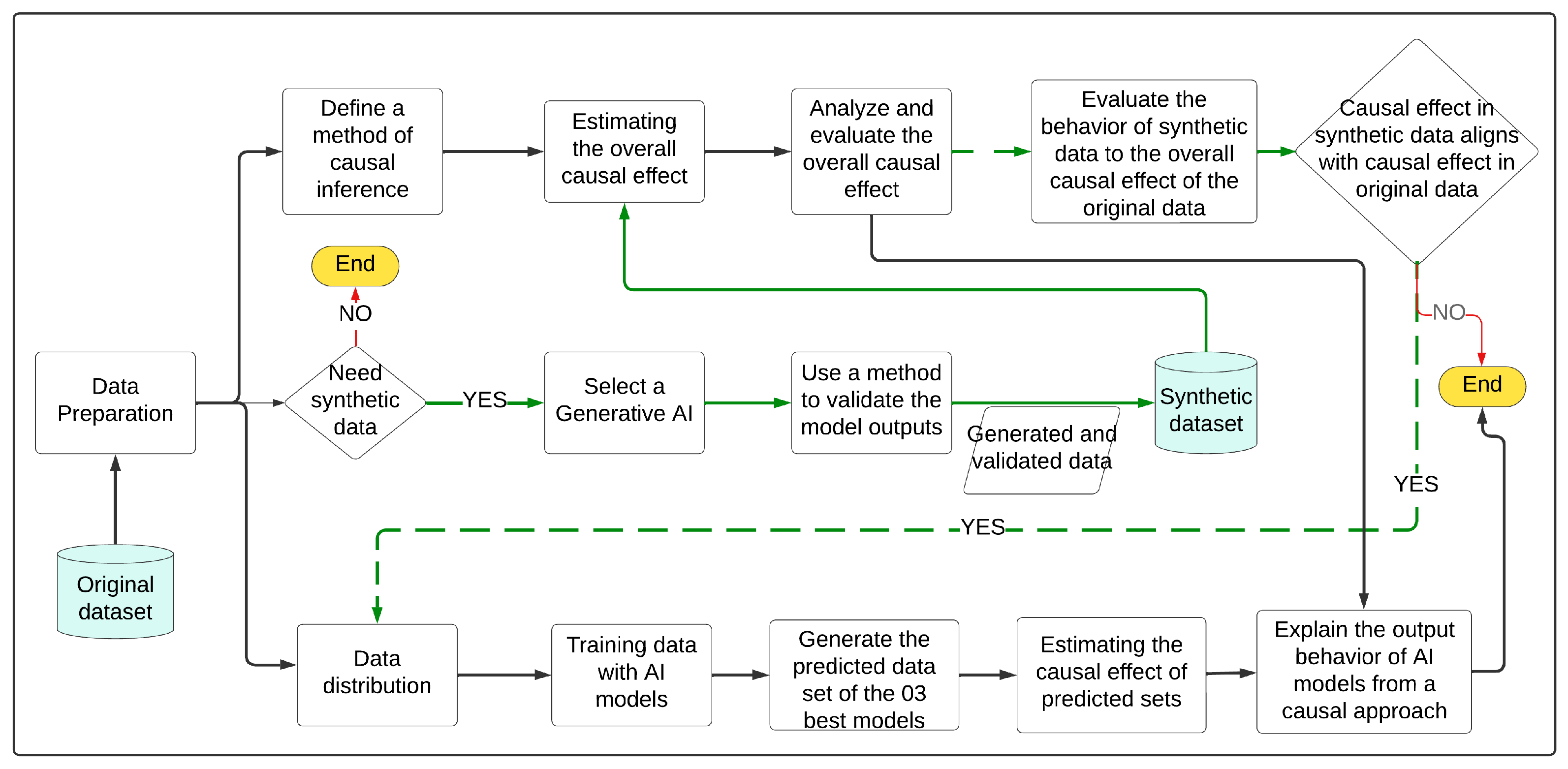
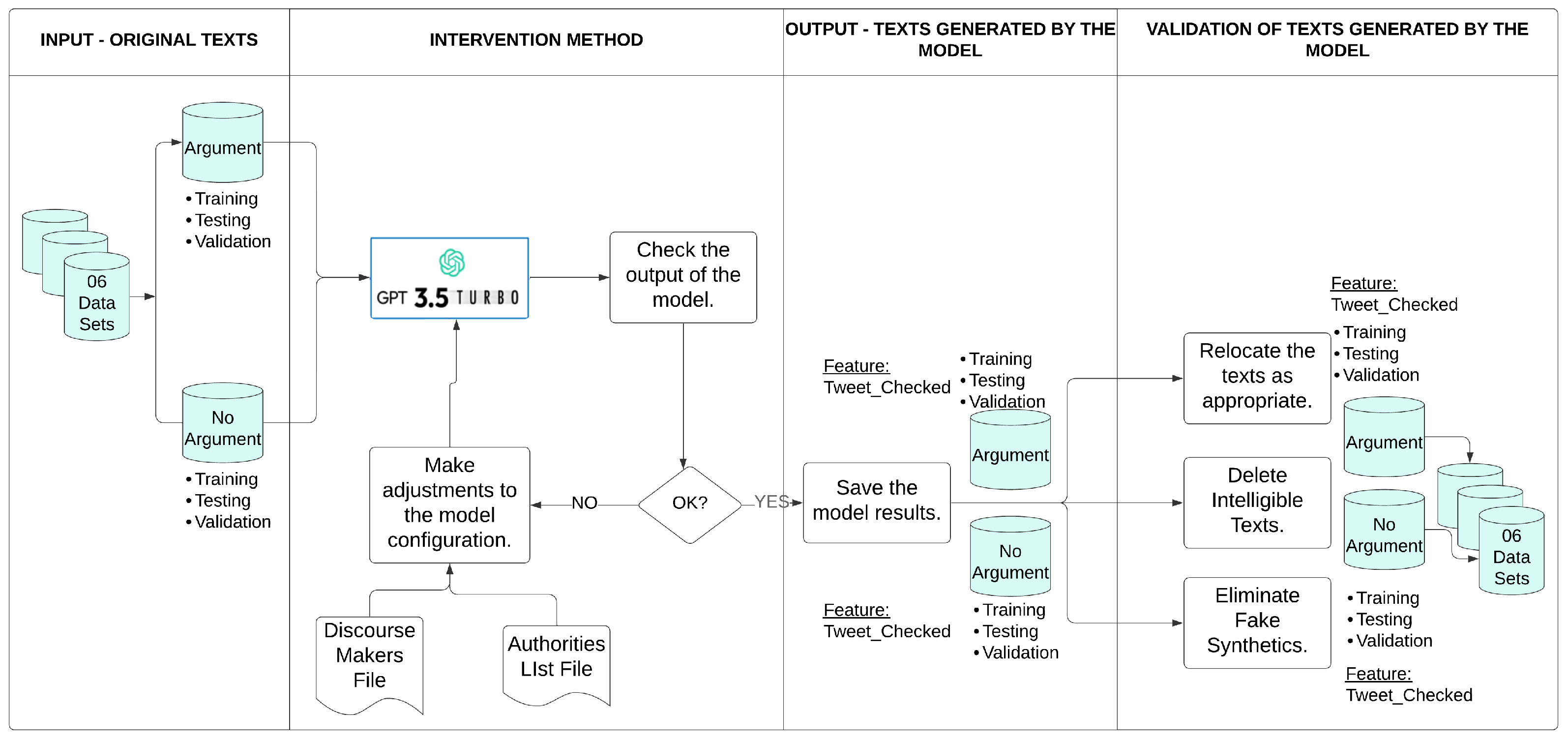

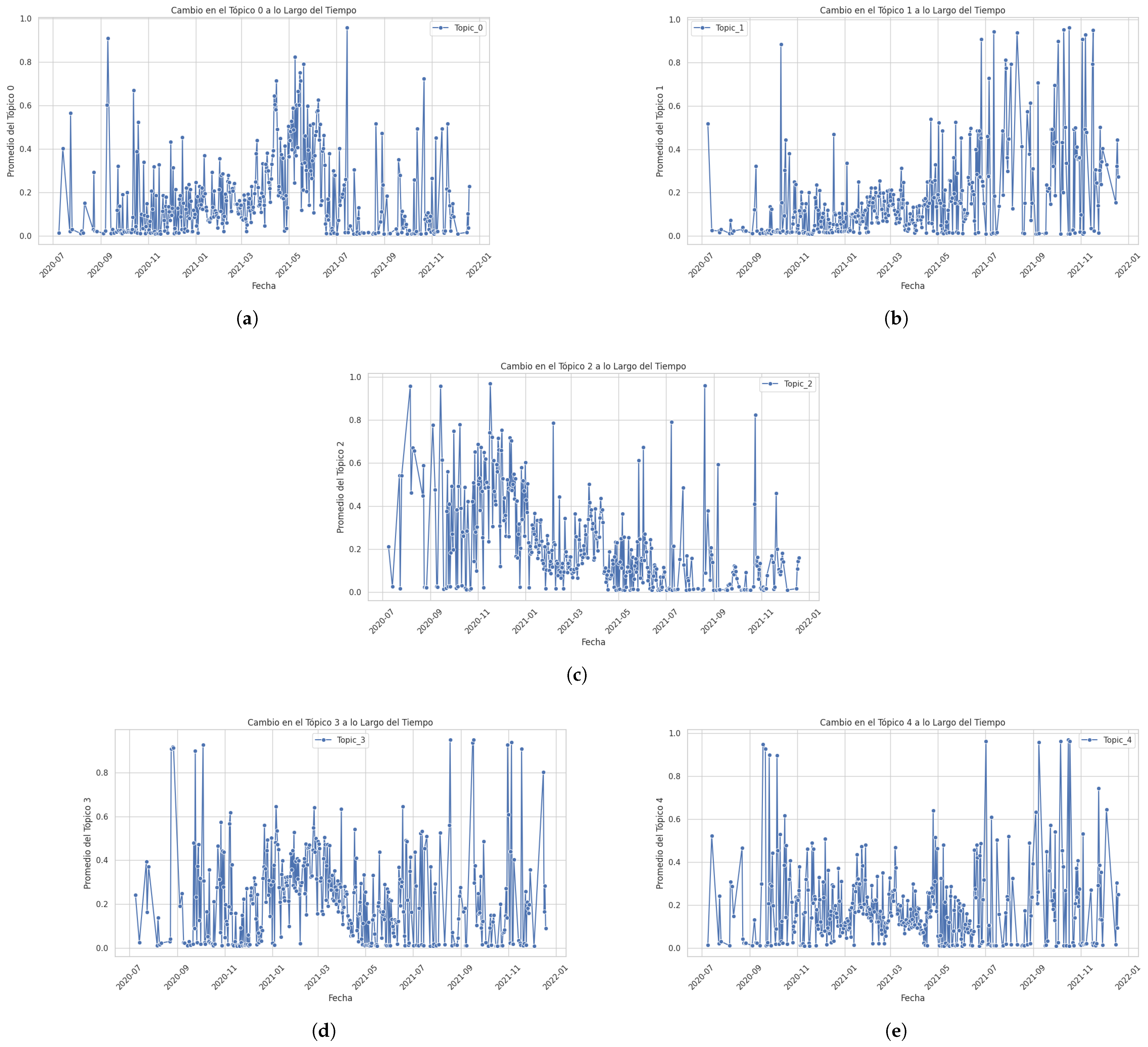
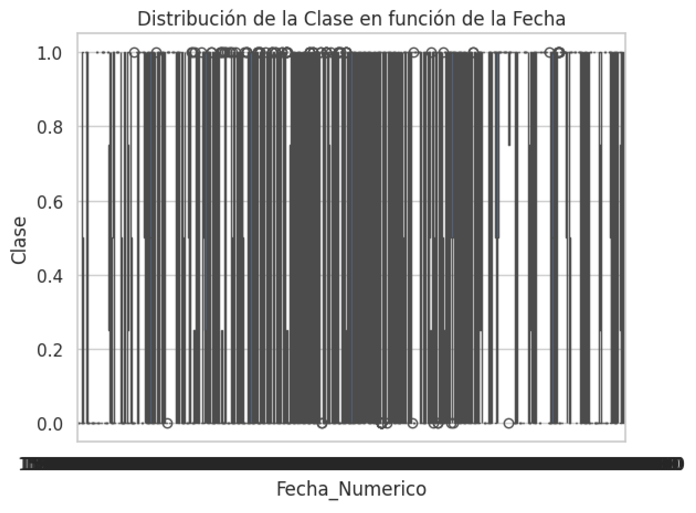
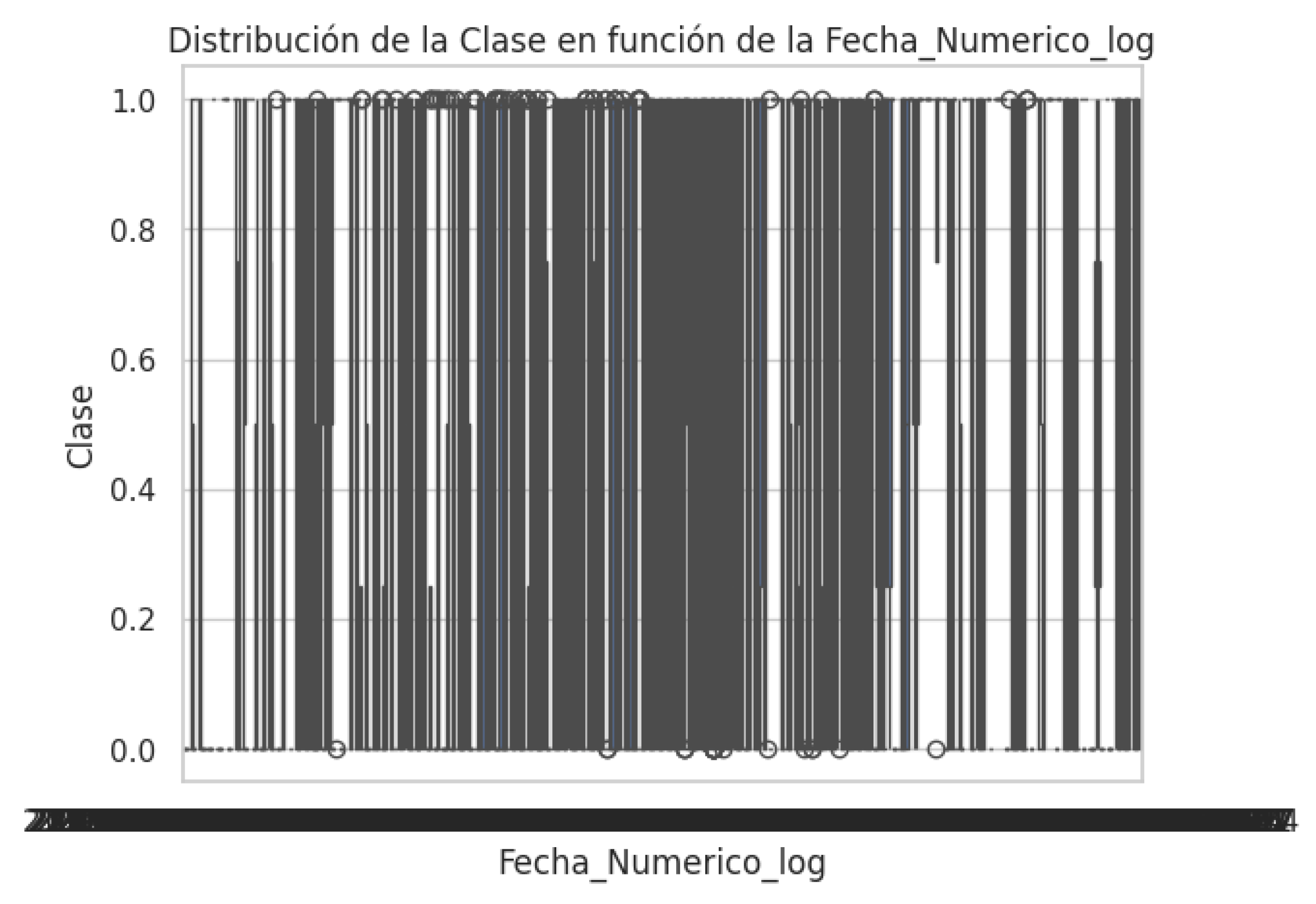
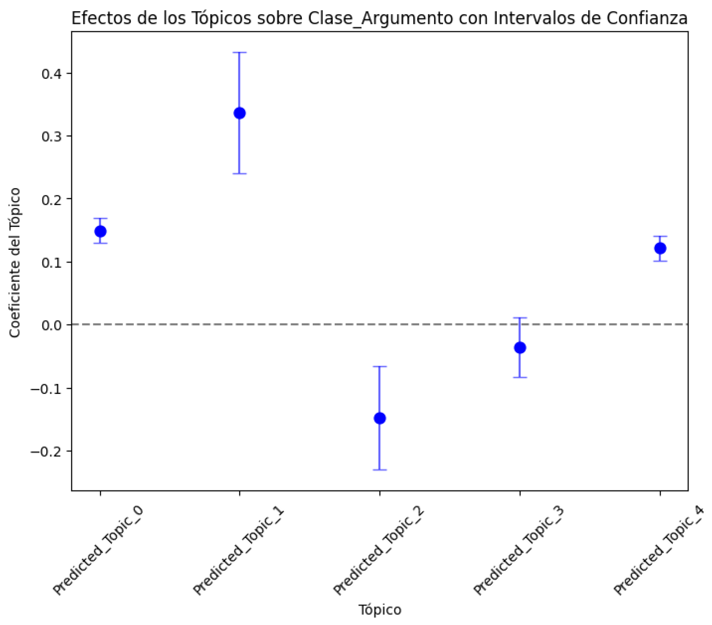
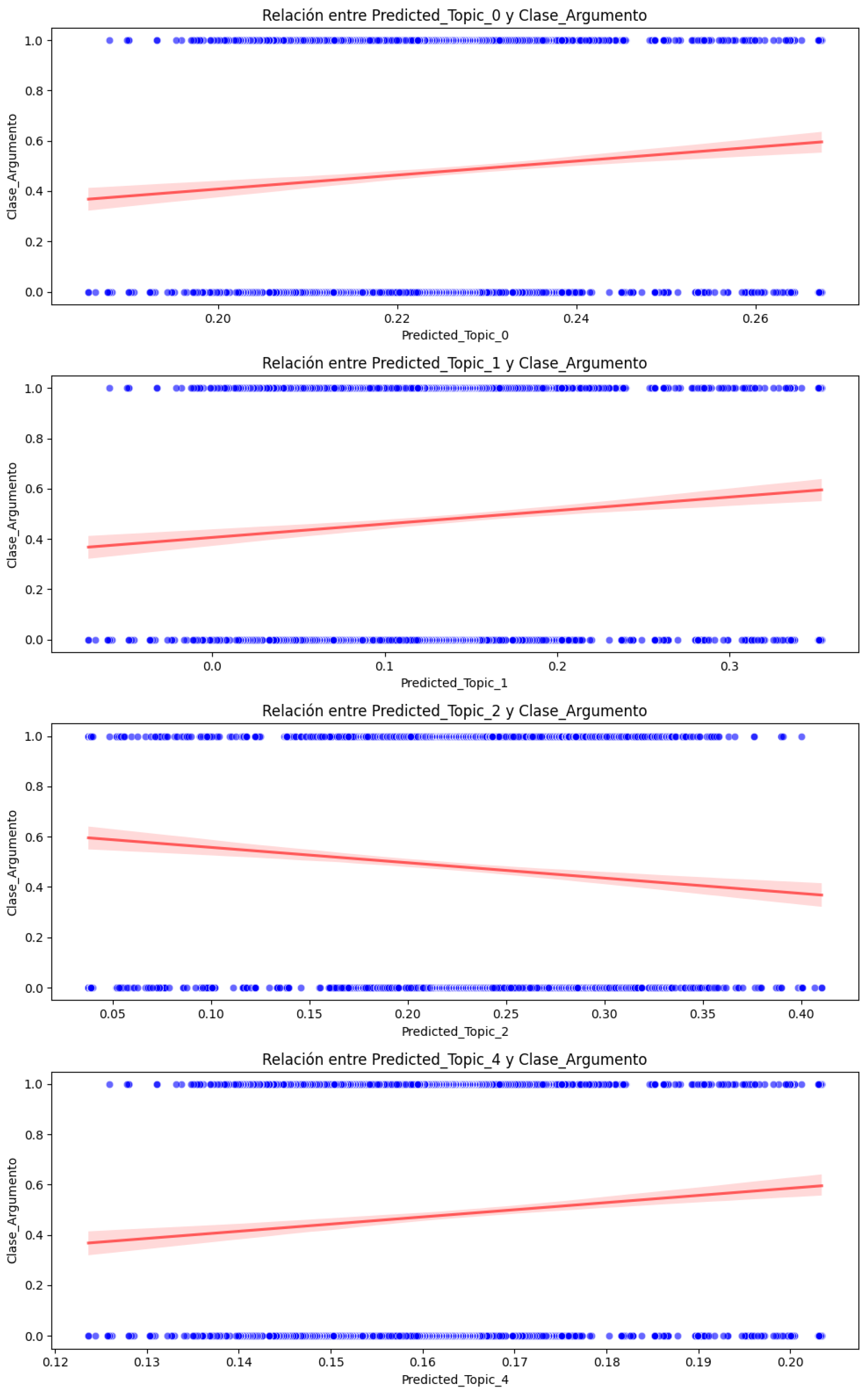

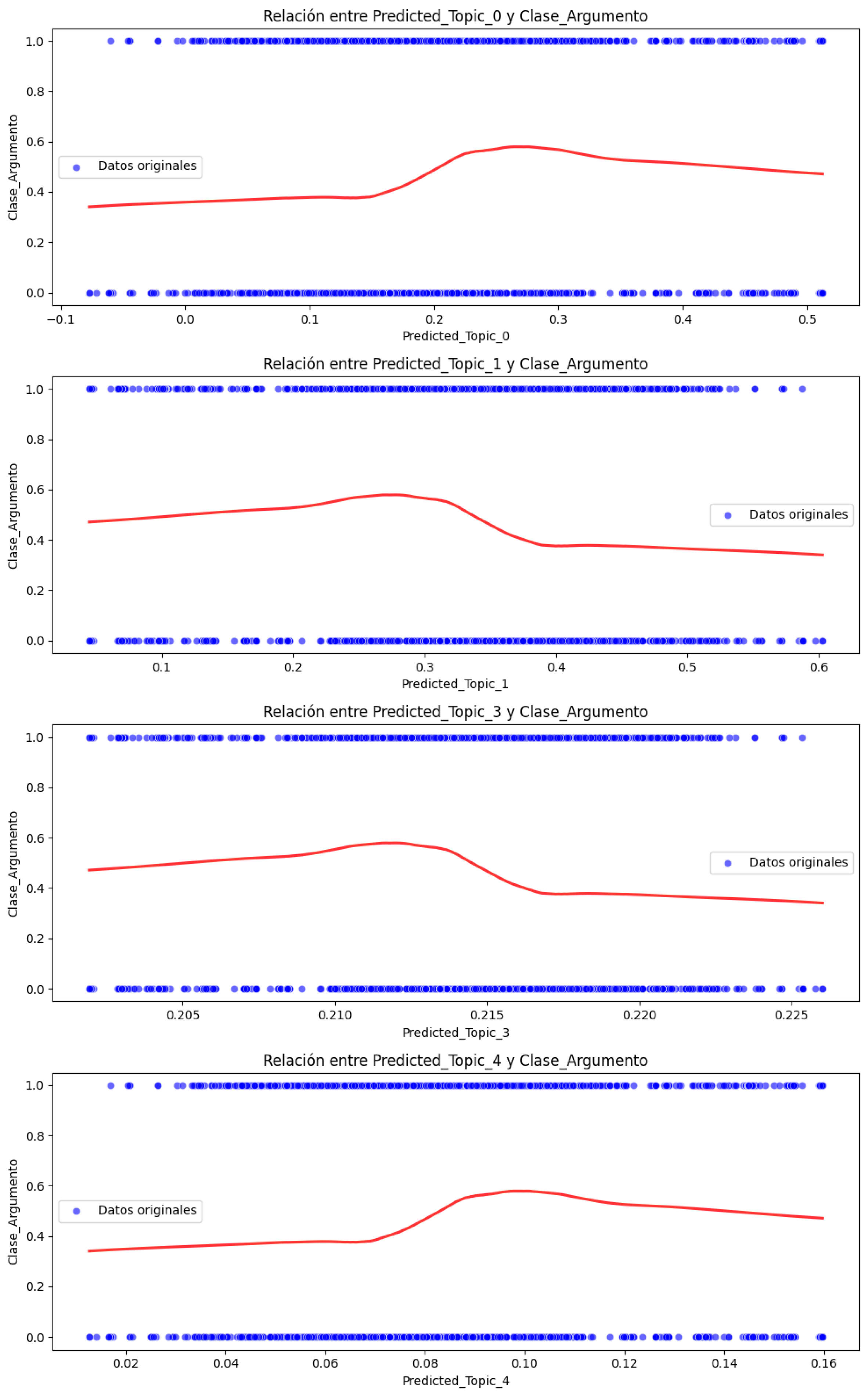
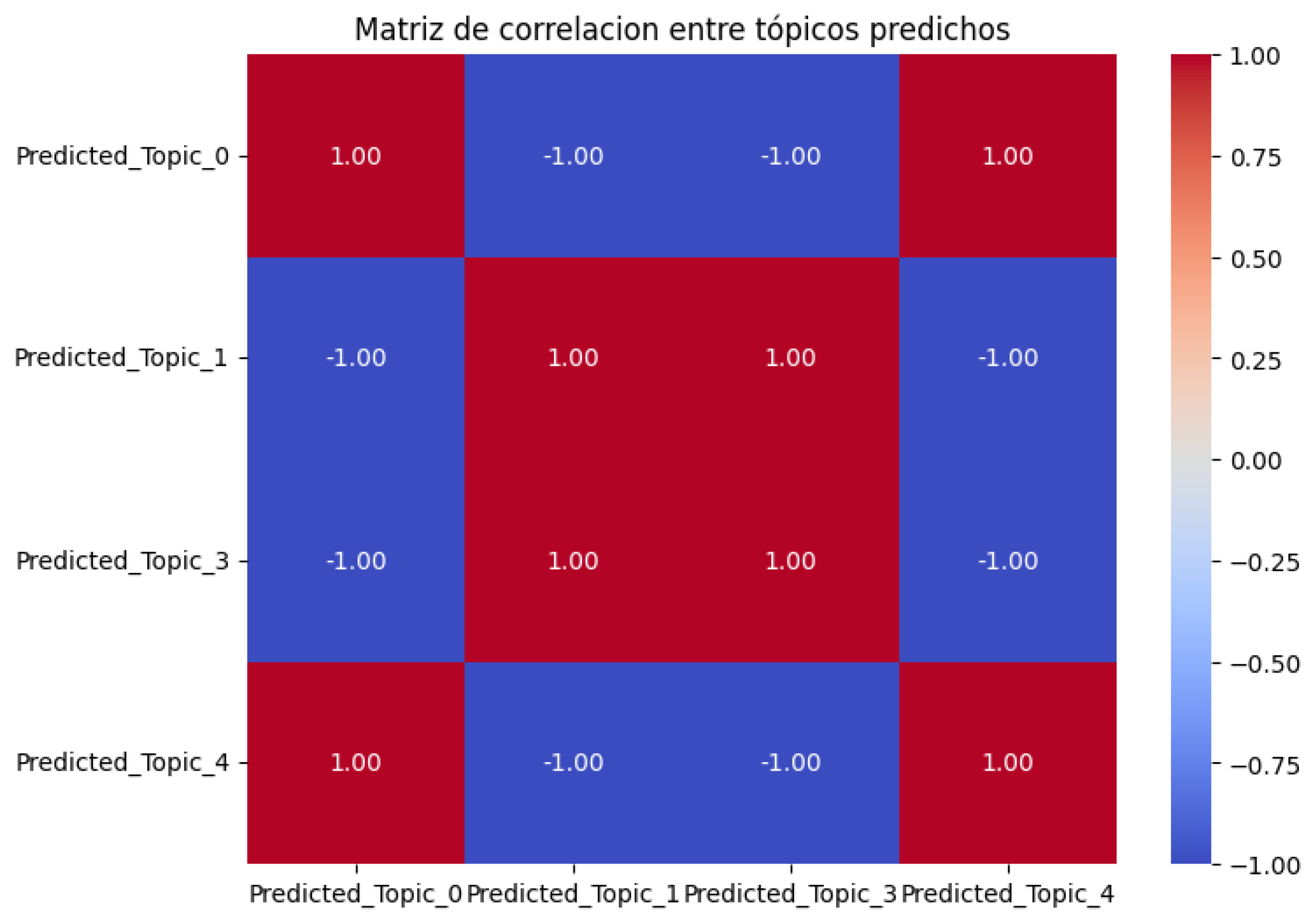
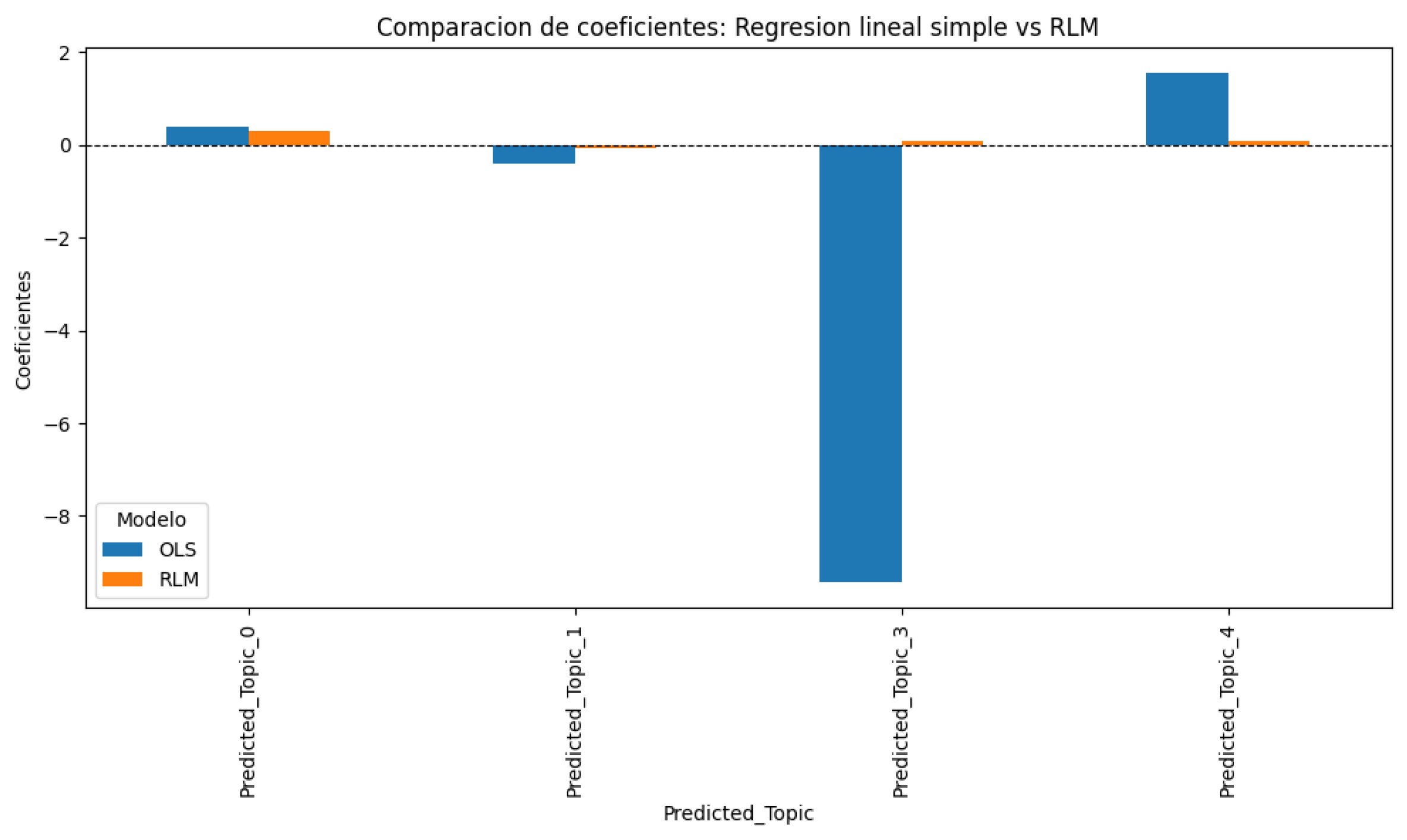

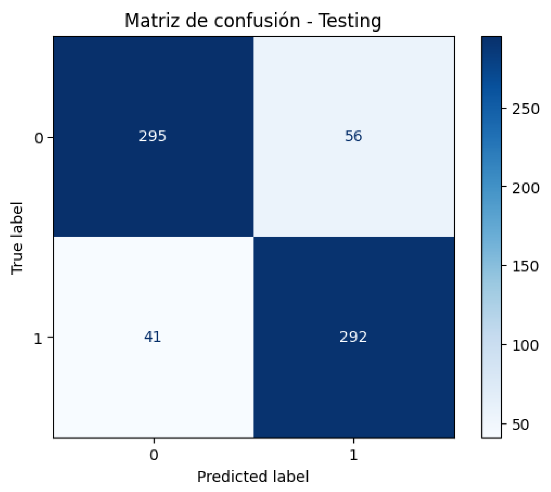

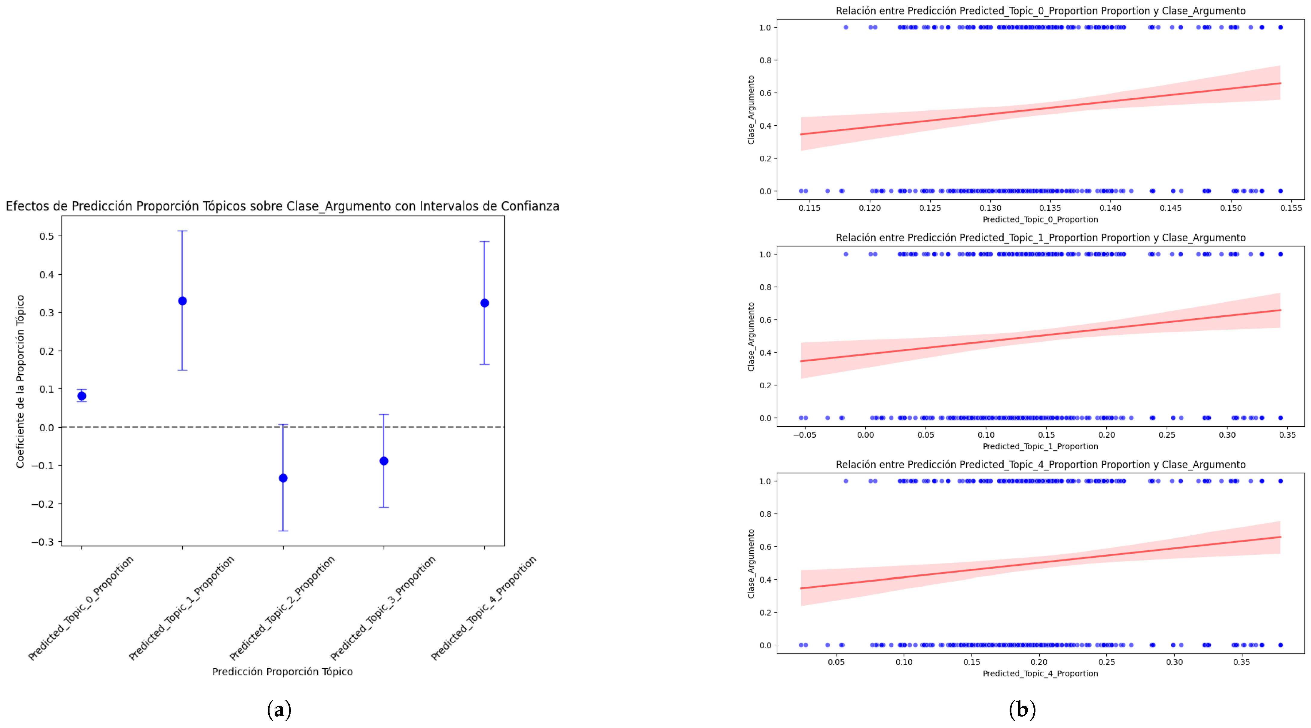
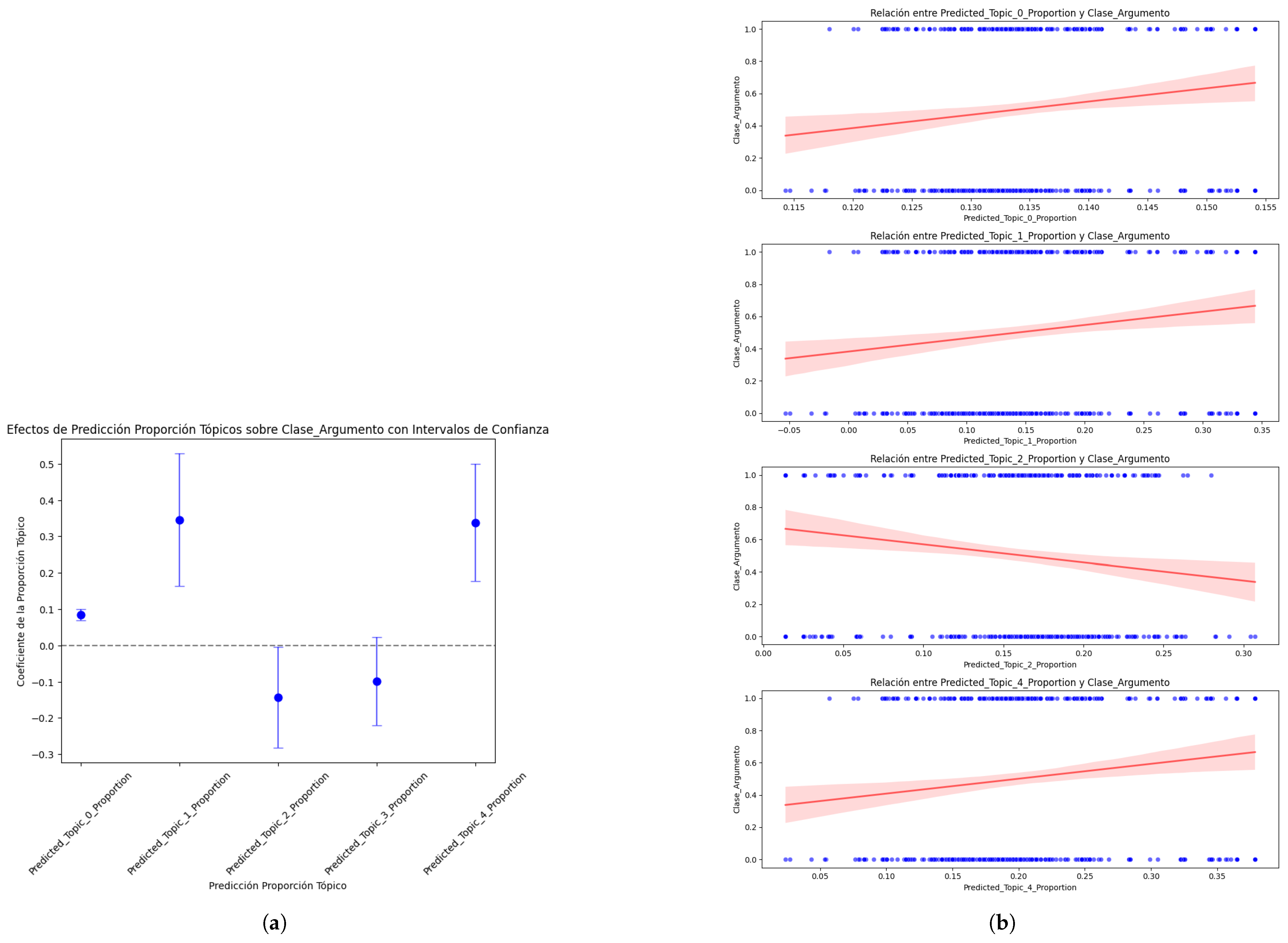
Disclaimer/Publisher’s Note: The statements, opinions and data contained in all publications are solely those of the individual author(s) and contributor(s) and not of MDPI and/or the editor(s). MDPI and/or the editor(s) disclaim responsibility for any injury to people or property resulting from any ideas, methods, instructions or products referred to in the content. |
© 2025 by the authors. Licensee MDPI, Basel, Switzerland. This article is an open access article distributed under the terms and conditions of the Creative Commons Attribution (CC BY) license (https://creativecommons.org/licenses/by/4.0/).