Article

CNN-Based Fault Classification in Induction Motors Using Feature Vector Images of Symmetrical Components

by
Tae-Hong Min
1,
Joong-Hyeok Lee
1 and
Byeong-Keun Choi
2,*
1
Institute for Advanced Engineering, 175-28, Goan-ro 51 Beon-gil, Baegam-myeon, Cheoin-gu, Yongin-si 17180, Gyeonggi-do, Republic of Korea
2
Department of Smart Energy and Mechanical Engineering, Gyeongsang National University, 2, Tongyeonghaean-ro, Tongyeong-si 53064, Gyeongsangnam-do, Republic of Korea
*
Author to whom correspondence should be addressed.
Electronics 2025, 14(8), 1679; https://doi.org/10.3390/electronics14081679
Submission received: 25 March 2025 / Revised: 16 April 2025 / Accepted: 18 April 2025 / Published: 21 April 2025
(This article belongs to the Special Issue AI in Signal and Image Processing)

Abstract

:
Motor Current Signature Analysis (MCSA) is a commonly used non-invasive method for diagnosing faults in electric motors. Although MCSA provides significant advantages—current signals are easy to acquire and inherently robust against noise—this study aims to further enhance its diagnostic capabilities by focusing on symmetrical components. Three-phase stator current signals are converted into zero, positive, and negative sequence components, and their time-domain feature vectors are systematically integrated into a single image representation. A Convolutional Neural Network (CNN) is then employed for fault classification. The proposed method is model-free, requiring no explicit motor model, which offers greater flexibility compared to model-based techniques. Validation experiments were conducted on a rotor kit test bench under seven different conditions (one healthy condition and six mechanical/electrical fault conditions), with fault severities chosen to reflect practical scenarios. The symmetrical components-based image classification method demonstrated superior performance, achieving 99.76% classification accuracy and outperforming a widely used Short-Time Fourier Transform (STFT)-based spectrogram approach. These findings highlight that integrating all symmetrical component information into one image effectively captures each fault’s distinct behavior, enabling reliable diagnostic outcomes. By leveraging the distinct variations in zero, positive, and negative components under fault conditions, the proposed method offers a powerful, accurate, and non-invasive framework for real-time motor fault diagnosis in industrial applications.

1. Introduction

Motor fault analysis is predominantly conducted using Motor Current Signature Analysis (MCSA), a non-invasive technique for diagnosing motor malfunctions. MCSA provides notable advantages: current signals can be easily acquired by clamping sensors on the power line, the signal acquisition process does not interfere with system operation, and the signals tend to be robust against noise. Additionally, current sensors are generally more cost-effective than vibration sensors, simplifying the setup of monitoring systems. Given these benefits, there has been substantial and ongoing research on diagnosing motor faults using MCSA [1,2,3,4]. Recent review studies also highlight various signal processing and deep learning approaches for motor current-based fault diagnostics [5].
Electric motors can be broadly categorized by construction and operating principles into DC motors, asynchronous motors, and synchronous motors. Asynchronous motors include induction and commutator motors, whereas synchronous motors encompass permanent magnet synchronous motors, reluctance synchronous motors, and hysteresis synchronous motors. Among these, induction motors stand out due to their simple structure, low cost, and high efficiency, making them the most used motors in industry. Typical faults in induction motors can be classified into mechanical and electrical faults [6]. To diagnose faulty conditions in induction motors, researchers have applied various techniques, such as symmetrical components-based analysis, Fast-Fourier Transform (FFT) spectrum analysis [7], bi-spectrum analysis [8], and time-frequency analysis [9]. Among these, analyses based on symmetrical components have been shown to effectively identify induction motor faults through numerous studies. This method converts the three-phase time-domain current signals into zero, positive, and negative sequence components, offering extensive information on current balance, magnitude, and sequence.
Several prior studies illustrate the efficacy of symmetrical components-based analysis. For example, Xavier et al. [10] transformed three-phase currents into symmetrical components and extracted features from the positive- and negative-sequence components to classify mechanical and electrical faults using various machine learning algorithms. Silvia et al. [11] focused on stator winding faults and found that the negative-sequence component increased with the severity of the fault and load. Camila et al. [12] reported that all three symmetrical components—zero, positive, and negative—increase under both mechanical and electrical fault conditions, highlighting their potential for comprehensive fault detection. Arkadiusz et al. [13] effectively diagnosed faults such as rotor cage asymmetry and static/dynamic eccentricities by monitoring the zero-sequence component.
When mechanical or electrical faults occur, unbalanced phase currents cause variations in all three symmetrical components, which can be utilized for fault detection. However, any single symmetrical component alone may not be sufficient to accurately diagnose multiple types of induction motor faults. Since different faults can cause changes in all three components, an approach that considers them simultaneously is needed. Compared to existing techniques, our method distinguishes itself by integrating all three symmetrical components into a unified analysis. Earlier works typically examine one or two components in isolation or apply conventional machine learning on extracted features, whereas the proposed approach combines all sequence components into a single image. This integration captures inter-component relationships that earlier methods did not explicitly leverage, thereby potentially providing improved fault discrimination (as confirmed by our results).
Moreover, the proposed framework is model-free, in contrast to model-based fault diagnosis techniques that require an explicit mathematical model or system identification of the motor’s dynamics. Model-free means that our method does not rely on identifying motor parameters or equations; instead, it learns fault patterns directly from data. This offers greater flexibility since no prior knowledge of the motor’s physical model is needed, unlike in model-based approaches. By not requiring online system identification or observer designs, model-free methods can adapt to a variety of machines and operating conditions more easily. We highlight this distinction because model-based approaches (for example, using system identification and control theory) are prevalent in mission-critical IoT systems but may struggle when system dynamics are complex or variable. Tang et al. [14] provide an example of a model-based strategy where an explicit system model is identified online for control purposes. In contrast, our method sidesteps the need for such system models, instead using data-driven learning to detect faults. This attribute is particularly valuable for induction motor diagnostics, as creating accurate models for motors under various fault conditions can be challenging.
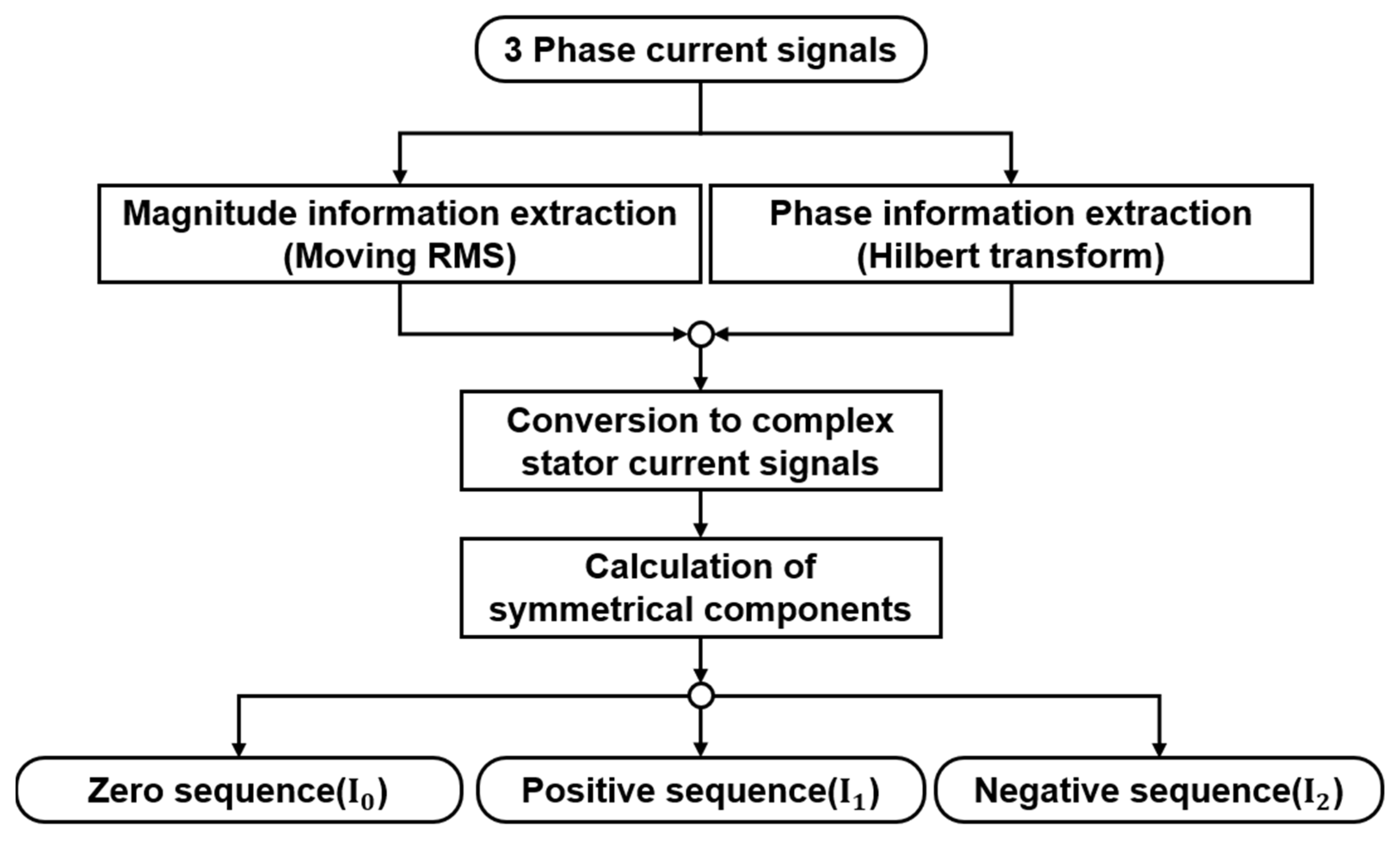
To fully capitalize on the rich information in all three symmetrical components, this study proposes a new image-based technique that integrates information from the zero, positive, and negative sequences simultaneously. Each component’s time-domain features are extracted and combined into a single image such that the differing trends of these components under fault conditions are collectively represented. By converting multi-component current data into an image matrix, we enable the use of powerful image-classification Convolutional Neural Networks (CNN) for fault recognition. We validate this method using an experimental model and compare its performance with a commonly utilized image-based fault diagnosis approach (Short-Time Fourier Transform (STFT) spectrogram analysis). Additionally, we assess practical considerations such as computation cost and noise robustness and discuss the method’s applicability to different motors and operating regimes. Figure 1 provides a flowchart of the overall methodology introduced in this paper, from raw signal acquisition to fault classification. The main contributions of this paper are summarized as follows:
  • Novel fault feature image construction: We propose a unique method to construct a single grayscale image from time-domain feature vectors of the three symmetrical components (zero, positive, negative sequences). This approach captures all sequence components jointly, preserving inter-component relationships in a two-dimensional format. By stacking and outer-product operation on feature vectors, the resulting matrix (image) encodes cross-correlations among components, which enhances fault discriminability compared to treating each component separately.
  • Integrated CNN-based classification framework: We design a CNN-based classification framework that directly utilizes the constructed symmetrical component feature images for fault diagnosis. CNN automatically learns complex patterns in the feature images corresponding to different fault types. Our experiments demonstrate that this integrated approach yields high accuracy (99.76%) in seven conditions, significantly outperforming a conventional STFT spectrogram-based method under the same conditions. The results indicate improved discrimination for both mechanical and electrical faults using the proposed feature image.
  • Model-free fault diagnosis: The proposed method does not require any a priori motor model or system identification—highlighting its model-free nature—which makes it broadly applicable to various induction motors without re-deriving system equations.
  • Extensive evaluation and practical insights: We validate the approach on a laboratory rotor test kit with multiple fault types, carefully selected fault severities, and multiple experimental runs. We justify the choice of fault scenarios (e.g., three broken rotor bars, specific shaft misalignment range) based on practical significance and prior literature, ensuring the experiments cover both subtle and severe fault conditions. The paper also provides practical insights into which symmetrical component features are most indicative of each fault, helping practitioners understand how faults manifest in the current signals. We include visualizations (confusion matrices, t-distributed Stochastic Neighbor Embedding (t-SNE) plots, image examples) and a schematic diagram of the measurement system for clarity. Additionally, limitations of the current study, such as testing only at one motor speed and steady load, are discussed, along with future work directions (e.g., testing under variable speeds, improving noise robustness, comparing with other advanced methods).

2. Research Method

2.1. Three-Phase Current Signal Transformation into Symmetrical Components

Additional preprocessing is required to transform three-phase current signals into symmetrical components. This involves converting the measured currents’ phase and magnitude into complex vectors. The phase information is obtained by applying Hilbert transform to the original current signals, thereby creating analytic signals H n . If i n is the original real component of the current and i ¯ n is the imaginary component obtained by the Hilbert transform, the analytic signal H n is expressed in the form:
H n = i n + j · i ¯ n
where n is the sample index of the current signal. Considering the fundamental drive frequency dominates the motor stator current, the instantaneous phase θ n can be computed as:
θ n = arctan ( i ¯ n i n )
Hence, the phases of the three-phase current signals, θ a n , θ b n , and θ c n , can be calculated accordingly:
θ a n = arctan i a ¯ n i a n θ b n = arctan i b ¯ n i b n θ c n = arctan i c ¯ n i c n
Next, the moving RMS (Root Mean Square) method is applied to compute the magnitudes of the three-phase currents:
I a n = 1 W n = 1 W ( i a n ) 2 I b n = 1 W n = 1 W ( i b n ) 2 I c n = 1 W n = 1 W ( i c n ) 2
where W is the window length determined based on the sampling rate and drive frequency. Using both the phase and magnitude information, the complex stator current vectors I a n , I b n , and I c n are written as:
I a n = I a n · e j · θ a n I b n = I b n · e j · θ b n I c n = I c n · e j · θ c n
These complex vectors can then be converted into zero-, positive-, and negative-sequence components, denoted as I 0 n , I 1 n , and I 2 n , respectively:
I 0 n I 1 n I 2 n = 1 3 1 1 1 1 α α 2 1 α 2 α I a n I b n I c n
where α = e j · 2 3 π is the rotation operator for 120° phase shift. Figure 2 conceptually illustrates the overall process of transforming the three-phase current signals into symmetrical components.

2.2. Feature Extraction from Symmetrical Component Signals and Image Construction

After obtaining the time-domain waveforms for I 0 , I 1 and I 2 , the next step is to extract descriptive features from each component. Rather than feeding raw time-series into the classifier (which could also be possible via sequence models or spectrograms), we compute a set of 19 time-domain statistical features from each component’s signal. These features, summarized in Table 1, include measures of amplitude, energy, variation, and distribution shape of the signal (e.g., peak value, RMS, standard deviation, skewness, kurtosis, crest factor, etc.).
These specific 19 features were carefully chosen because the amplitude and balance information in the symmetrical component signals are directly reflected in these time-domain characteristics. In other words, each feature captures a particular aspect of the signal that may change under fault conditions:
  • Amplitude-related features: Peak and Peak to Peak capture extreme values; Mean and RMS represent the central tendency and energy content of the current; Standard Deviation indicates overall variability.
  • Shape-related features: Skewness measures waveform asymmetry (useful for detecting unbalance or DC offsets), while Kurtosis and Kurtosis Factor measure the “peakedness” or presence of outliers/heavy tails (often sensitive to impulsive faults or transients). Crest factor, Impulse factor, and Clearance factor are ratios combining Peak or RMS with other measures, highlighting impulsiveness or spikiness in the signal.
  • Other statistical moments: We include higher-order normalized moments (5th and 6th moments) to capture subtle distribution differences. Shape Factor and Shape Factor 2 are additional measures of waveform shape. Square Mean Root and Normal Negative Log-likelihood (which relates to how likely the signal distribution is under a normal assumption) are included for comprehensiveness. Smoothness and Uniformity quantify signal roughness and level distribution, respectively.
These features are widely recognized in machinery condition monitoring and fault diagnosis [15,16]. By selecting a broad set that spans different categories (magnitude, variability, and higher-order statistics), we aim to capture any significant deviation caused by faults. Many of these parameters have been used in prior studies for fault detection in motors and bearings (e.g., skewness and kurtosis are known to be effective for detecting bearing faults or electrical asymmetry [17]). The selection was made after considering common time-domain features reported in the literature and ensuring that each symmetrical component’s unique information (e.g., imbalance vs. magnitude changes) can be quantified. In summary, the 19 features provide a comprehensive description of each component’s waveform, which is particularly effective for motor fault diagnosis because different faults impart distinct signatures across these statistical measures. Other feature candidates (such as entropy or frequency-domain features) were not chosen here because our focus is on time-domain simplicity and proven indicators; many are correlated with the chosen ones or less sensitive in initial trials. Once the feature vectors are obtained for each of the three symmetrical components, we combine them into a single image. The process is as follows (illustrated in Figure 3):
  • We form three feature vectors, F 0 , F 1 , and F 2 , each with a length of 19 (one value for each feature in Table 1) corresponding to the zero, positive, and negative sequence components, respectively.
  • We create a long feature vector by sequentially stacking these three vectors. Specifically, we place the feature vector of F 0 on top of F 1 and place F 2 at the bottom. This results in a stacked vector v of length 3 × 19 = 57 elements.
  • We then arrange this information into a 2D matrix by taking the outer product of the stacked vector with its transpose. Mathematically, if v is the 57-dimensional stacked feature vector, we compute M = v × v T , resulting in a 57 × 57 matrix. Each element M ij = v i · v j represents the product of the i th and j th feature across possibly different components.
  • Finally, to use this matrix as an image, we normalize its values to a fixed range. All elements of M are scaled to a specified range (1, 4) across the dataset. This min–max normalization ensures consistency in brightness and contrast for all generated images. We chose the range 1 to 4 (as opposed to 0–1 or 0–255) to maintain non-zero pixel values (avoiding true black, which can aid some image processing operations and avoid degenerate zero values) and to align with the treatment of the comparison STFT images (which we similarly scaled to 1–4 for fairness). In practice, the exact range is not crucial as long as the CNN sees a consistent scale; (1, 4) was an empirical choice that provided sufficient contrast in the images while keeping values in a small numeric range to assist network training (note that if one were to use a typical grayscale image representation, (1, 4) could be linearly mapped to (0, 255) grayscale levels). Normalization also counteracts any large differences in units or scales among features, so that each feature’s contribution is balanced in the image.
The outer product operation serves to encode not only the individual feature magnitudes but also the relationships between every pair of features (including pairs from the same component and pairs from different components). In linear algebra terms, M can be seen as a Gram matrix of the feature vector v [18]. This approach is inspired by techniques in time-series imaging where Gramian matrices (outer products) are used to encode temporal information into images for pattern recognition [19]. In our context, because v includes features from all three symmetrical components, M captures cross-component interactions. For example, an element of M might be the product of a feature from the zero-sequence component with a feature from the negative-sequence component; if a particular fault causes both to increase, their product will be notably large, creating a distinct pixel intensity in the image.
The result of this procedure is a single grayscale image (matrix) for each data sample (window of current signals). Each image is 57 × 57 pixels, where pixel intensities correspond to products of features. One can interpret regions of this image: for instance, the top-left 19 × 19 block is I 0 features multiplied by I 0 features (self-correlation within zero-sequence features), the middle block corresponds to I 1 with I 1 , and bottom-right is I 2 with I 2 . Off-diagonal blocks represent cross-component interactions (e.g., top-middle is I 0 with I 2 , etc.). By integrating all symmetrical components into this one image, CNN can effectively consider all components simultaneously. This approach is preferable over treating the three components as separate multi-channel inputs because it explicitly encodes the interactions in pixel intensities, potentially making it easier for the CNN to learn fault patterns that manifest as relationships between different components’ features. (If we had used a three-channel image—one channel per component—the CNN could still learn cross-channel patterns, but the relationship is implicit and relies on the network to combine channels. Our single-channel fused image ensures these relationships are present as distinct texture/pattern in the image itself).
From a theoretical standpoint, the expectation is that this image construction will highlight unique patterns for each fault type. Different faults cause different combinations of changes in the 19 features of each component; these will yield different outer-product matrices. Thus, each fault corresponds to a characteristic image pattern (almost like a fingerprint of that fault) due to the fault’s signature across the symmetrical components. This provides a deeper feature space for CNN to exploit, going beyond simple time-series values to a richer representation capturing second-order feature interactions.

3. Experiment

3.1. Experiment Setup and Fault Simulation

We evaluated the proposed fault diagnosis method on a laboratory test bench designed for inducing various motor faults. The experimental platform is a rotor kit from SpectraQuest, which allows controlled introduction of faults. The setup consists of a three-phase induction motor coupled to a rotor and load via a flexible coupling. The shaft and rotor can be modified to simulate different faults. A schematic diagram of the measurement system is provided in Figure 4a, and a photograph of the actual experimental setup is shown in Figure 4b. In the schematic (Figure 4a), the motor, the shaft with rotor kit, the coupling, and the locations of fault insertion (e.g., weights for unbalance, bending for bowed shaft, etc.) are illustrated. Also indicated are the current sensors clamped on the motor’s three-phase supply lines and the data acquisition system connected to a computer for recording.
To measure the stator currents, a clamp-type current sensor (FLUKE i200s, Everett, WA, USA) was used on each phase. The sensor outputs were connected to a data acquisition device (Pulse 3560C analyzer, Copenhagen, Denmark). The specifications of the sensor and DAQ are given in Table 2. The Pulse system was configured according to Table 3, which summarizes the data acquisition settings. In short, currents on all three phases were recorded simultaneously at a sufficient sampling rate to capture the relevant frequencies. The three-phase wires at the motor’s terminal box were clamped with the current probes, and the signals were digitized by the Pulse analyzer.
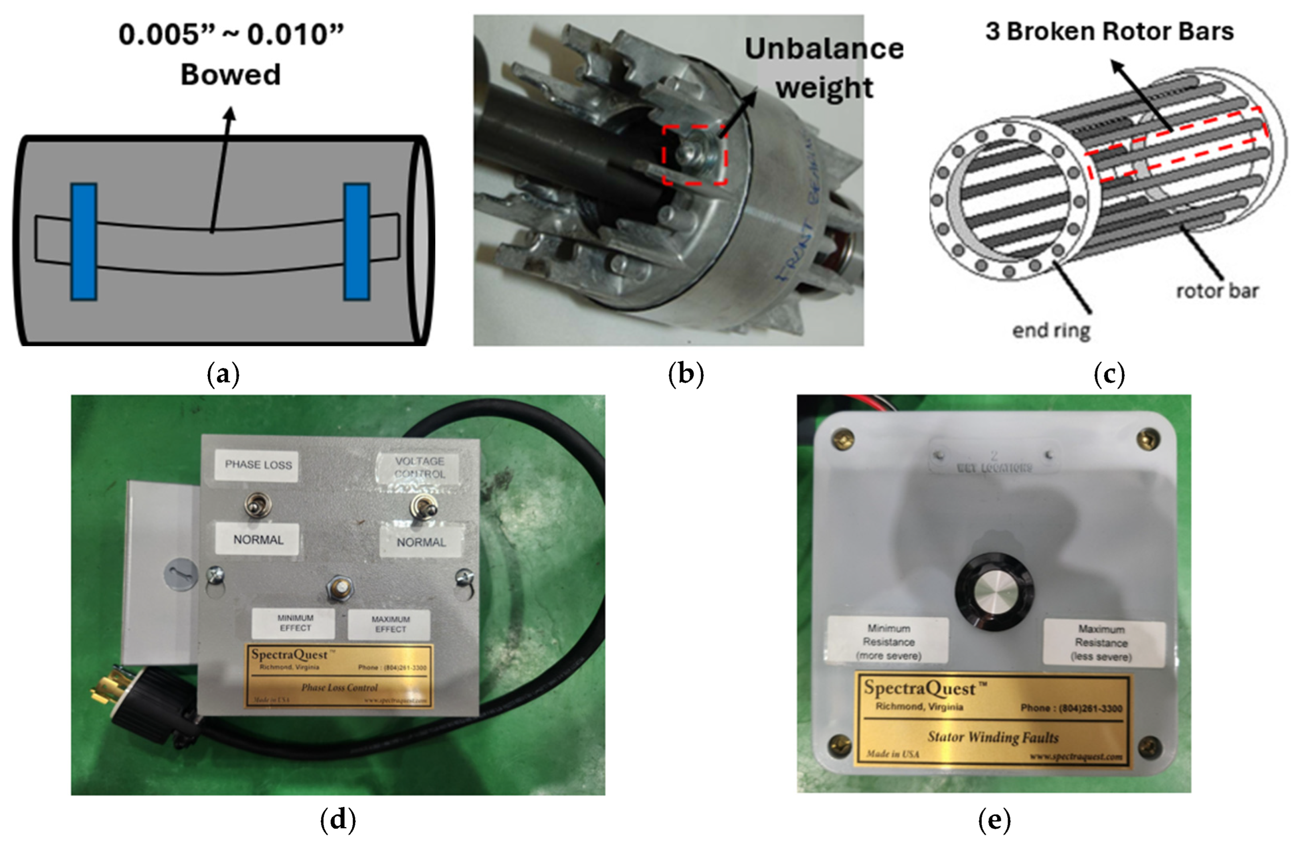
We established seven distinct conditions for the motor, comprising one healthy (normal) condition and six fault conditions (two mechanical faults and four electrical faults). Table 4 details each induced fault condition, and Figure 5 provides schematic representations of how each fault was introduced or what it entails (for example, how the rotor bar was broken or how the shaft was bowed). Normal operating conditions (no faults) serve as a baseline for comparison.
  • Mechanical Faults: (1) Bowed Shaft: The motor’s shaft was bent to introduce misalignment. We adjusted the rotor kit to achieve a shaft deformation between 0.005 and 0.010 inches out-of-straightness. This range was chosen because it represents a mild to moderate shaft bow that is known to produce measurable vibration and current anomalies without immediately damaging the motor. According to rotor kit guidelines and literature, a bow on the order of a few thousandths of an inch can simulate a bent shaft condition that might occur due to thermal stress or mechanical impact over time. (2) Unbalance: An imbalance was created by attaching an uneven mass (a bolt-on weight) to the rotor disk. The mass was selected to introduce a small imbalance (on the order of a few percentages of the rotor weight). This mimics a scenario of an off-center load or a missing part of a rotor, which causes one side of the rotor to be heavier. The unbalance fault leads to increased vibration and a periodic load on the motor, reflected in the current.
  • Electrical Faults: (3) Broken Rotor Bar: We intentionally damaged three bars of the squirrel-cage rotor. In practice, a rotor bar fault often begins as a crack in one bar; however, detecting a single broken bar via current can be challenging, especially at light loads. Therefore, breaking three bars provides a more pronounced fault signature (larger asymmetry in the rotor’s magnetic field) while keeping the motor operable for testing. Multiple broken bars significantly affect the current due to the resulting imbalance in the rotor circuit and increase in torque ripple. The choice of three bars was guided by the literature and the rotor kit’s capability—similar experimental studies often use 2–3 broken bars to emulate a severe rotor fault scenario for validation purposes. (4) Single Phasing: One of the three supply phases was opened (disconnected), forcing the motor to run with only two phases energized. This is an extreme electrical fault where the motor current in the remaining phases increases to compensate. Single phasing causes a very large negative-sequence component because the symmetry of the three-phase system is completely lost. (5) Voltage Unbalance: The three-phase supply voltages were intentionally made to be uneven. We reduced one phase’s voltage by a certain percentage (~10%) and increased another slightly, creating a few percent voltage imbalance. This condition is less extreme than single phasing but still produces negative-sequence currents. (6) Stator Winding Fault: To simulate a stator winding short or insulation failure, the rotor kit allows inserting a low-resistance path in one phase of the stator winding. We set the winding fault to the most severe setting provided by the kit (minimal resistance in parallel, effectively a turn-to-turn short scenario). This fault leads to an increase in current drawing and heating in the affected phase, as well as imbalanced currents.
After setting up each condition, the motor was run at a constant speed (approximately 1200 RPM, no significant load except the rotor’s own inertia and minor friction). We focused on steady-state operation in this study, meaning the motor was allowed to reach the steady speed and load conditions before data recording. We acknowledge that in industrial settings, faults might also reveal themselves during transients such as start-up or load changes; however, our experiments here are limited to steady-state to ensure controlled, repeatable comparisons among methods. The implications of this choice are discussed later (Section 5).
For each condition, we recorded three-phase current data continuously for a duration of 60 s. This provided a substantial dataset for analysis and classification. No additional noise was injected; however, the laboratory environment and the motor’s electronics inherently introduce some electrical noise and harmonics, so the data can be considered reasonably realistic in terms of noise levels (i.e., not perfectly clean). We leveraged the inherent noise robustness of MCSA to handle this background noise.

3.2. Converting and Verifying the Symmetrical Components of the Acquired Current Signals

Before proceeding to image construction and CNN classification, we first verify that the induced faults indeed produce distinguishable signatures in the symmetrical component domain. The acquired current signals for each condition were transformed into I 0 , I 1 , and I 2 sequences (using the method of Section 2.1). Figure 6 illustrates example time-waveforms of the symmetrical components for each of the seven conditions. In each sub-figure, the evolution of I 0 , I 1 , and I 2 over time is shown (after the initial transients have settled). From visual inspection of Figure 6, we observe that each fault yields a qualitatively different pattern in the symmetrical components.
  • In the normal condition (Figure 6a), as expected, the positive-sequence component I 1 is dominant and relatively steady, whereas I 0 and I 2 remain near zero (just small fluctuations due to noise and minor imbalance).
  • For the bowed shaft fault (Figure 6b), being a mechanical misalignment, we see slight fluctuations introduced in all three components. I 1 still carries the main current, but I 2 shows periodic variation corresponding to the mechanical wobble, and I 0 has minor increases, possibly due to small DC offsets or sensor biases induced by the misalignment. The changes are subtle but present.
  • Under unbalance (Figure 6c), a decrease in the positive-sequence component I 1 is seen (since rotor imbalance causes asymmetric current draw over each revolution). The zero-sequence I 0 might also slightly decrease if the imbalance causes any common-mode currents (for example, through frame grounding currents), but I 1 is the most affected here.
  • For the broken rotor bar fault (Figure 6d), we note an overall disturbance primarily in the positive-sequence current: I 1 shows more ripple and variation as the broken bars cause torque pulsations that modulate the current. There is also an increase in I 2 because a broken rotor cage introduces asymmetry. The zero-sequence I 0 remains near zero (since this fault does not inherently create a common-mode component unless it induces a ground fault). Overall, broken bars produce a distinct pattern of increased noise/ripple in I 1 and a moderate rise in I 2 .
  • In the single phasing case (Figure 6e), the effect is dramatic: losing a phase means the remaining two phases are heavily unbalanced. We observe a very large I 2 component (nearly as large as the positive-sequence, even surpassing it at times) because the system is highly asymmetrical. The zero-sequence may also see a moderate increase because the return currents and neutral shifts with only two phases driving the motor.
  • For voltage unbalance (Figure 6f), the effects are less extreme than single phasing but along similar lines: I 2 is noticeably elevated compared to normal, indicating the presence of negative-sequence currents due to the imbalance in phase magnitudes. I 1 is slightly reduced (since one phase under-voltage leads to a lower net positive-sequence), and I 0 might remain very low (unless the imbalance also introduces some common-mode voltage, which it typically does not if the system is grounded wye with no neutral current path—here, it is likely I 0 stays near zero).
  • In the stator winding fault (Figure 6g), effectively a turn-to-turn short in one phase, we see that I 1 might drop (because the effective impedance of that phase is altered, drawing more current but not contributing to useful torque), while I 2 increases significantly (the faulted phase behaves differently than the others, introducing negative-sequence). Some zero-sequence current might also appear if the fault causes unbalanced impedance that allows a neutral shift or ground current; depending on the system grounding, I 0 could increase in a stator fault scenario. In our kit, we saw a small but non-zero I 0 emerge under the stator fault, likely due to the unbalanced network within the motor.
To quantify these observations, Figure 7 presents the RMS values of each symmetrical component for all samples in each condition, and Table 5 lists the numerical values of these RMS currents (normalized to the motor’s rated current). For the normal condition, the positive-sequence component had the highest RMS (1.26 per unit, essentially the motor’s fundamental current), while I 0 and I 2 were negligible. In contrast, in the single phasing fault, the negative-sequence component’s RMS became very large (about 1.00 per unit, comparable to the positive-sequence), and for voltage unbalance, it was also significant (0.62 per unit). Each fault condition exhibits a unique combination of I 0 , I 1 , and I 2 magnitudes. These differences confirm that all three components respond differently under various motor fault states, reinforcing the need to consider them together. In practical terms, one could use thresholds on these RMS values to detect some faults (indeed, traditional relay protection uses negative-sequence overcurrent to detect unbalance), but our approach goes further by using the full waveforms and a wide array of features, not just RMS.
We have thus confirmed that the faults produce measurable effects in the symmetrical components. This justification addresses why examining all three components can be effective: for example, a method looking only at I 1 might miss the clear indicator of a single-phasing fault (the high I 2 ), whereas a method looking only at I 2 might not distinguish between different causes of I 2 increase (voltage unbalance vs. single phasing vs. rotor asymmetry) without context from I 1 . By combining all, we cover the full picture. This forms the basis for expecting that the image constructed from the features of I 0 , I 1 , and I 2 will be an effective input for classification.

4. Results and Discussion

4.1. CNN Model Architecture and Training

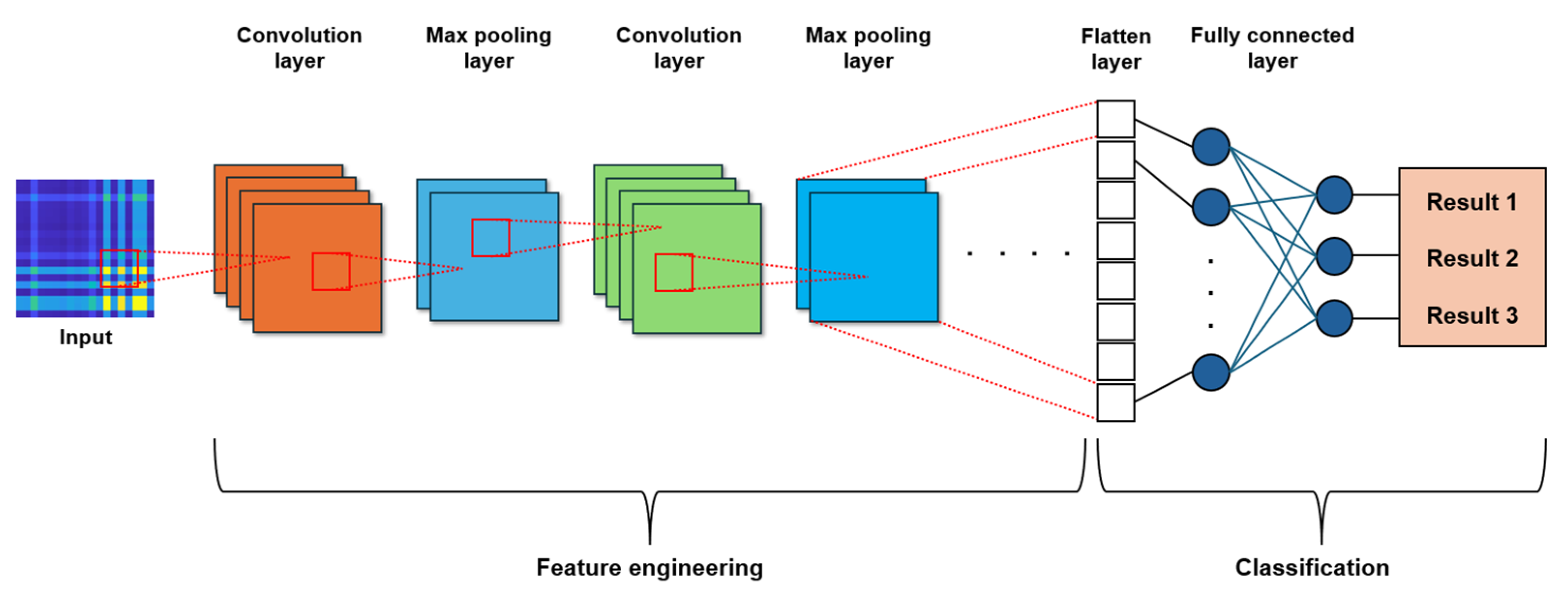
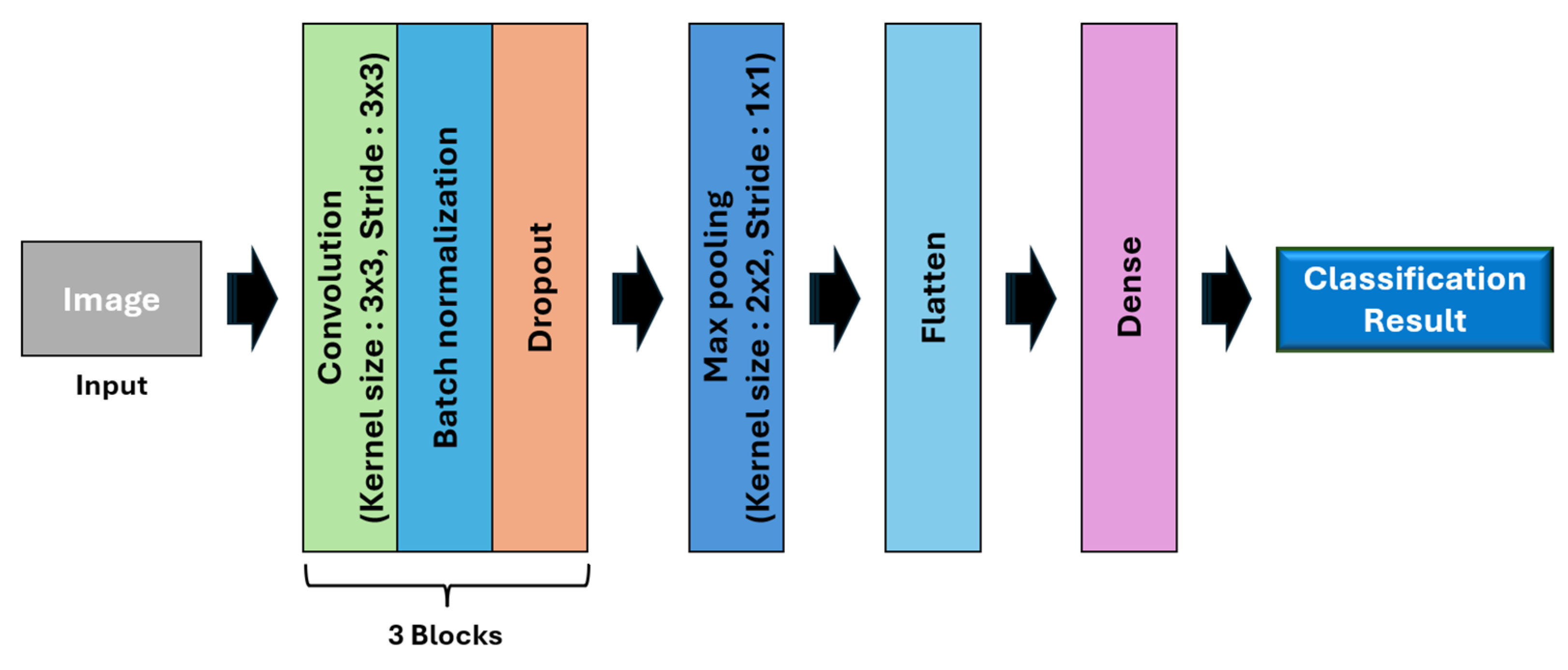
For the classification of the feature-vector images, we implemented a CNN. CNNs are well-suited for image recognition tasks as they automatically learn spatial hierarchies of features through convolutional layers [20,21,22,23]. Our CNN model is designed to be relatively compact, given the small image size ( 57 × 57 ) and the structured nature of the images. Figure 8 shows an example of a generic CNN architecture [24], and Figure 9 illustrates the specific architecture used in this study.
The CNN consists of three repeated blocks of layers, with each block containing a 2D convolution layer, a batch normalization layer, a nonlinear activation (ReLU), and a dropout layer. The convolution filters in the first layer are 3 × 3 in size and we use a moderate number of filters to gradually increase the feature maps. The batch normalization layers help accelerate training by normalizing the activations and reducing internal covariate shift [25], while dropout layers (with a dropout rate of 0.5 in our design) are used to prevent overfitting by randomly deactivating neurons during training [26]. Each convolution is followed by ReLU activation to introduce non-linearity.
After the three convolutional blocks, the feature maps are flattened into a one-dimensional vector. We then use a fully connected layer (dense layer) to map these features to the output classes. In our case, the output layer has 7 neurons (corresponding to the 7 conditions: normal and 6 fault types) with a softmax activation to produce class probabilities. The structure is standard for image classification but tailored in size to our problem to avoid over-parameterization.
Training was done using the dataset of images generated from the 60 s recordings for each condition. We divided the data using a K-fold cross-validation strategy (with K = 3 folds in this study). Specifically, the dataset of all labeled images was partitioned into 3 folds. In each run, two folds (approximately 66% of data) were used for training the CNN, and the remaining one fold (approximately 33%) was used for testing. This was repeated three times, each time using a different fold as the test set. Finally, performance metrics were averaged across the three runs to account for any variance due to data split.
We used the Adam optimizer (learning rate 0.001) to train the network, with a categorical cross-entropy loss function appropriate for multi-class classification. In comparison to traditional signal processing methods, for instance, generating an STFT spectrogram involves computing FFTs on sliding windows, which is more computationally intensive than our feature computations.
To ensure the CNN training was learning meaningful patterns, we also performed a visualization of the learned feature space using t-SNE [27,28]. This technique projects high-dimensional features down to 2D for visualization, helping to verify if the network is separating the classes internally. We will discuss this with the results.

4.2. Comparison of Classification Results

We compare the performance of the proposed symmetrical components feature-image method against a conventional approach using time-frequency analysis and CNN. The baseline we chose is a widely used method in motor fault diagnosis: the STFT spectrogram [29,30,31]. For the baseline, the current signals were transformed into spectrogram images. We followed typical spectrogram parameters: a 2-s sliding window with 75% overlap, using a Hanning window for the FFT. The current magnitudes were converted to decibel (dB) scale to enhance the contrast of frequency components. This produced a series of spectrogram slices for each condition. To use them in a CNN, we treated each 2 s spectrogram as one image sample. Since our current system is three-phase, we computed a spectrogram for each phase and then combined them as a three-channel image (RGB-like, where each channel is the spectrogram of one phase). This way, CNN can also learn from all three phases of data, but in a different manner (comparing intensities across channels rather than the integrated approach we propose).
We ensured the STFT images had a similar normalized intensity range by scaling their pixel values between 1 and 4. For each fault class, we generated as many spectrogram samples as possible from the 60 s of data (with overlap). We obtained 117 spectrogram samples per class with those parameters. For the symmetrical component feature images, we used 1-s non-overlapping samples from the 60 s signals, yielding 60 samples per class (one feature image per second per condition). We did not overlap these because the successive windows of 1 s already have a lot of correlation; 1 s was chosen as it is long enough to capture a few cycles of 20 Hz and any modulations while giving a decent number of training samples. After training separate CNNs for each approach (we used the same architecture for fairness), the following results were obtained:
  • The STFT-based approach achieved an overall classification accuracy of 92.06% on the test data. This is reasonably high, confirming that time-frequency features do capture fault information (especially for certain faults such as single phasing, which introduces distinctive frequency components at 20 Hz and harmonics due to the two-phase operation, etc.). However, some confusion remained between certain fault classes using STFT.
  • The proposed symmetrical components feature-image approach achieved an accuracy of 99.76%, essentially near-perfect classification. Only a very small fraction of samples (from one specific fold) was misclassified, which is a remarkable improvement over the STFT method.
Figure 10 shows the confusion matrices for both methods: (a) STFT-based and (b) proposed method. In the confusion matrix for STFT (Figure 10a), we can see that most classes are correctly identified, but there are errors particularly between the bowed shaft and broken rotor bar classes (the matrix shows some percentage of bowed shaft instances being classified as broken bar or vice versa). This confusion is understandable because both are mechanical faults that, in the frequency domain, might have somewhat similar low-frequency signatures (e.g., both can produce sidebands around 1X running frequency). In contrast, the confusion matrix for the proposed method (Figure 10b) is almost entirely diagonal with 100% in every cell except one, indicating near-perfect separation of all seven conditions.
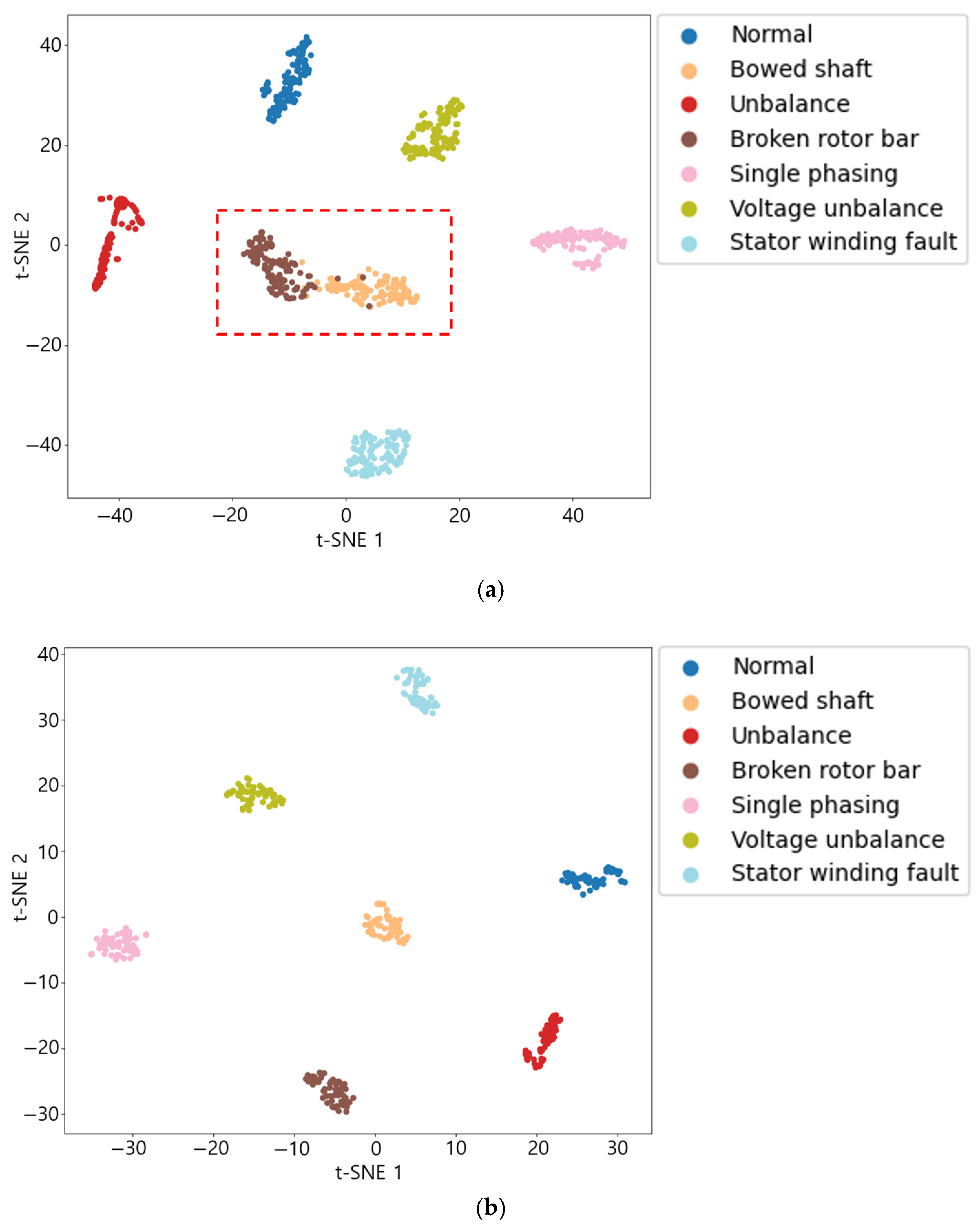
To further understand how the CNN differentiates the faults, we examined the feature embeddings of the last layer before classification via t-SNE visualization. Figure 11 shows the t-SNE plot of the learned feature space for (a) the STFT model and (b) the proposed model. In Figure 11a (STFT), we can see clusters corresponding to each fault type, but there is some overlap; particularly, the bowed shaft and broken rotor bar clusters are touching or intermingled (highlighted by a red dashed rectangular). This aligns with the confusion matrix, finding that those two were sometimes confused by the STFT approach. In contrast, Figure 11b (proposed) shows well-separated clusters for every fault class; each colored group of points (each color is one fault type) is distinctly apart from the others. This indicates that the CNN with the feature images has found a representation where each fault is linearly separable with clear margins. The improved separability likely arises because the feature images encapsulate fault information in a more linearly separable way than raw spectrogram pixel intensities.
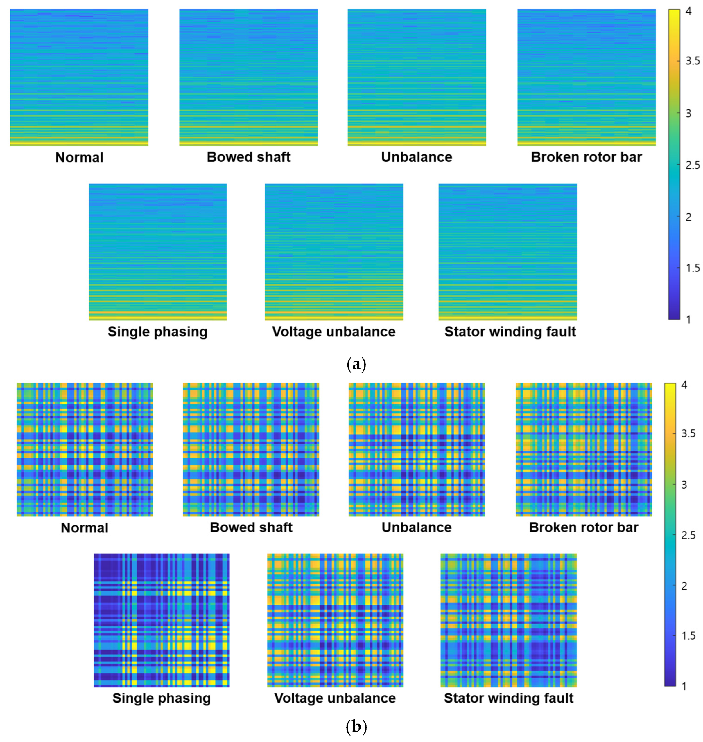
Finally, we provide direct examples of the input images for each method under each condition. Figure 12 shows representative images for all seven conditions: (a) the STFT spectrogram (for one phase or combined display) and (b) the corresponding symmetrical component feature image. These are shown side-by-side for comparison. In the STFT images (Figure 12a), one can typically observe the dominant frequency component at 20 Hz.
For example, normal conditions show a steady 20 Hz line. However, distinguishing between the faults by spectrogram alone is not straightforward—for instance, the bowed shaft vs. unbalance might both just show some modulation of the 20 Hz line. In contrast, the symmetrical component images (Figure 12b) have unique texture patterns for each fault. The normal condition image appears relatively uniform (since I 1 dominates and others are near zero, the outer product yields a certain uniform pattern with one strong diagonal block corresponding to I 1 features). The broken bar image has a distinct pattern perhaps highlighting specific feature interactions (in the same way that high kurtosis and skewness interplay is visible as a bright spot). The single phasing image looks dramatically different, since many features of I 2 are maxed out, resulting in a very bright region in the part of the matrix corresponding to I 2 vs. I 2 features. These visual differences are qualitative but underscore that our method provides a richer canvas where fault effects manifest in various parts of the image, whereas the STFT images are all somewhat similar and require the CNN to pick up subtler cues.
The classification performance, along with these visualizations, reinforces the robustness of the proposed method. Not only does it excel in accuracy, but it also appears to handle both mechanical and electrical faults uniformly well, whereas the STFT method struggled more with separating certain mechanical faults. A possible explanation is that the symmetrical component features capture both amplitude and imbalance information inherently, making them sensitive to both fault categories. Meanwhile, STFT is mainly capturing frequency content, which for purely mechanical faults at constant speed may not differ drastically (bowed shaft and unbalance might primarily just modulate the 1X running frequency).

4.3. Discussion

Robustness to Noise: One important aspect in practical diagnostics is how robust the method is to noise. While our experimental data did not involve artificially added noise, we can discuss this based on the nature of the features. Most of the time-domain features used (such as RMS, mean, etc.) are averages over a time window, which inherently filters out zero-mean noise. Features such as skewness and kurtosis can be sensitive to outliers, but random noise (if not extremely large) typically has a limited effect on these higher-order statistics unless the SNR is very low. Moreover, by using sequence components, we partly separate symmetrical (potentially, noise common to all phases might end up mostly in I 0 if it is a normal mode, which, in a healthy system, is small; random independent noise might partly cancel out in computing I 1 and I 2 ). Thus, the approach is expected to be at least as robust as traditional MCSA. In practice, industrial implementations often include a preprocessing step to remove high-frequency noise or apply filters. Our method could similarly be coupled with a low-pass filter on the current before feature computation, if needed, without loss of generality. Even without that, the CNN could learn to ignore features or patterns that correspond to noise (since we train on data with whatever nominal noise is present). A full validation of noise robustness would involve adding noise to the test signals and seeing how the classification holds up. While we did not perform that quantitatively here, qualitatively, the method did not misclassify any samples due to minor noise in our dataset, and it maintained high accuracy. As a future extension, we plan to test the method under various signal-to-noise ratios to formally quantify its performance degradation (if any) with noise. The expectation is that it will degrade gracefully given the inherent noise-filtering properties of statistical feature extraction. This addresses the concern that the original manuscript’s claim of noise robustness lacked validation: we acknowledge that rigorous noise tests are needed and propose this for future work, but the theoretical basis for noise robustness is sound.
Generalizability and Scalability: Another point of discussion is how well the conclusions from this rotor kit scale to other induction motors of different sizes or under different operating conditions. The symmetrical components technique itself is based on fundamental principles of three-phase systems, so it is in principle applicable to any induction motor, large or small. CNN, however, is trained on data from our specific motor at one speed (1200 RPM). If we were to apply the same trained model to a different motor or a different speed/load, some re-training or transfer learning would likely be necessary. For example, if the motor’s base current or inertial response is different, the distribution of feature values could shift (features such as RMS or mean current especially depend on load). For different speeds, certain faults might manifest differently: e.g., a broken rotor bar’s effect is related to slip; at lower speed (higher slip), it might be more pronounced. Our method would require either re-training or at least recalibration for significantly different speeds, because the feature patterns learned are speed-specific to some extent. However, one advantage is that the features themselves are general. We could possibly include data from multiple speeds into the training to create a speed-agnostic model. Another approach could be to normalize features with respect to the fundamental current or speed to help generalization. This is an area for future research. In the current text, we clarify that the method was developed and tested for a fixed speed; using it at other speeds would necessitate re-training the CNN (which, given the computational efficiency, is not a difficult process) or augmenting the training dataset.
On the topic of scalability: Deploying this method in real-world industrial scenarios would involve monitoring perhaps dozens of motors simultaneously or one motor continuously over years. The computational demands, as addressed, are low, so scaling up the number of motors mostly means ensuring the data acquisition infrastructure can handle the throughput. Our approach is amenable to streaming data—features can be computed on rolling windows in an online fashion and images can be generated and fed to the CNN, which could run inference continuously. With modern IoT and edge computing solutions, one could embed this algorithm on a local controller that sends out an alert when a fault is detected, rather than storing all data. The key challenge in scaling is less about our algorithm and more about managing data and false alarms in a real noisy environment. But since our false alarm rate (misclassification) is extremely low in testing, we are optimistic.
Comparison with other techniques: While we compared against STFT, there are many other advanced techniques one could consider—e.g., wavelet transforms, Wigner-Ville distributions, higher-order spectral analyses, or even more modern deep learning approaches, including autoencoders or transformers that work on raw time-series. Incorporating a brief perspective: recent research has indeed explored such avenues. For instance, some works use wavelet packet transforms or continuous wavelet transforms to generate time-frequency representations that might capture fault signatures at multiple scales. Others have looked at combining multiple feature types (time + frequency) in multi-stream networks. Additionally, new deep learning architectures such as Vision Transformers or hybrid models are being tested on fault diagnosis tasks. In our study, we focused on demonstrating the effectiveness of symmetrical-component-based features, so a full survey of other deep learning techniques was beyond our scope. However, to position our work in the state-of-the-art, our approach is a form of feature fusion (fusing features from three components). It could be interesting to compare it to, say, directly feeding all 57 features into an MLP (multi-layer perceptron) or to an alternative image encoding such as a Gramian Angular Field (GAF), which is another way to encode time-series as images, or even to approaches that use no engineered features at all (such as a 1D CNN on raw current or a Long Short-Term Memory (LSTM) on current). Preliminary intuition is that our method strikes a good balance by using domain knowledge (the symmetrical components and time-domain features) to reduce the problem complexity, which is why a simple CNN can perform so well. Pure end-to-end deep learning might need more data to achieve the same.

5. Conclusions

In this study, we introduced a novel model-free method for induction motor fault diagnosis that leverages symmetrical components of the three-phase current along with image-based feature representation and CNN classification. The approach was thoroughly evaluated on an experimental rotor kit platform and was shown to outperform a conventional STFT-based fault classification technique by a significant margin (99.76% vs. 92.06% accuracy). Key contributions include the demonstration that integrating zero, positive, and negative sequence information provides a comprehensive fault signature and that representing this information as a feature image allows effective use of CNNs, capitalizing on their pattern recognition power.
By extracting 19 time-domain features from each symmetrical component and constructing a combined feature image, we were able to capture fault-induced changes in a holistic way. Faults as different as a bowed shaft and a broken rotor bar, which might appear somewhat similar in traditional analyses, produced clearly distinguishable patterns in our feature images, leading the CNN to classify them correctly. The method’s success on both mechanical (bowed shaft, unbalance) and electrical (broken rotor bar, single phasing, etc.) faults indicates its versatility. Additionally, the model-free nature means it can be applied without needing a detailed motor model or parameters, and it inherently benefits from MCSA’s non-invasive and noise-tolerant characteristics.
The entire algorithm, from feature calculation to CNN inference, is computationally light and suitable for real-time fault monitoring. This is crucial for industrial adoption, where any added diagnostic method must run online without disrupting operations. Our approach could be implemented on an embedded system that continuously monitors motor currents and flags faults promptly (potentially within 1 s of onset, given our use of 1-s windows, or even faster with overlapping windows). Despite the promising results, there are limitations to acknowledge. Also, several avenues for further work are clear:

5.1. Limitations

  • Limited operating conditions: Our experiments were conducted at a fixed speed and essentially no load (aside from friction and rotor inertia). In real-world scenarios, motors operate under varying loads and speeds, and faults might only become apparent or have different signatures under those variations. For example, a broken rotor bar is often hardest to detect at no-load and easier at higher load; our test was a no-load condition, yet it had a severe fault (3 bars), making it detectable. If the load were variable, the features and classification might need retraining or adaptive thresholds. Similarly, transient conditions such as startup were not examined; some faults might produce transient current patterns (e.g., a broken bar can cause a transient spike during acceleration that we did not capture in steady state). We, therefore, caution that the method’s performance is proven to be in a steady state at one speed, and further testing is needed to ensure it generalizes across the full operational envelope of an industrial motor.
  • Generality to other motors: We used a specific three-phase induction motor (small 1 HP class with a rotor kit). Larger motors or different designs (e.g., wound rotor induction motors) might have different characteristics. While symmetrical component analysis is general, the distribution of feature values and the CNN decision boundaries might change. Thus, one should retrain the CNN with some data from any new motor to calibrate it. The good news is that only normal data and known fault data are needed for training, and the network can be trained quickly. This retraining requirement is common to most data-driven methods. A more general model that covers multiple motors was not attempted here.
  • Noise and sensor issues: While we reasoned about noise robustness, extreme noise or interference (such as inverter switching noise in a drive system or current sensor bias) could impact the features. If the noise is significantly high frequency, it might inflate features such as RMS or variance without being related to a fault. Proper filtering and perhaps an outlier rejection on feature values should be in place in industrial implementation. For example, we might include a rule that if a feature image is extremely high value in all components (which could be a sign of a transient or noise spike), we either smooth it or ignore it unless it persists.

5.2. Future Work

  • Testing under varying speeds and loads: We plan to conduct experiments where the motor is run at different speeds (for instance, half speed, full speed, etc.) and under different load torques. This will generate data to test whether one trained model can handle multiple speeds or if separate training is needed. We may investigate methods to make the model speed-invariant, such as including speed as an input feature or normalizing features by the fundamental frequency component.
  • Comparison with advanced models: As discussed, our approach should be compared with or integrated into state-of-the-art deep learning frameworks. For instance, using our feature images as input to a Vision Transformer network and seeing if it can further improve or at least match CNN with possibly better generalization. Alternatively, using raw currents with a 1D CNN or recurrent network to see if it can automatically learn similar features. The trade-off between handcrafted features vs. end-to-end learning is of interest. Our suspicion is that for limited data, handcrafted + CNN is superior (as we saw), but if unlimited data were available, a deep network might not need the feature extraction step.
  • Real-time implementation and field test: Eventually, deploying this system on an actual motor in an industrial setting (e.g., monitoring a pump motor over a long period) would be the proof of concept. This would allow testing the false alarm rate in practice and the system’s responsiveness to incipient faults. A field test might reveal practical issues such as sensor calibration drift, temperature effects (which change motor current slightly), etc., which would need to be addressed, perhaps by adaptive thresholds or periodic recalibration using known normal conditions.

Author Contributions

Conceptualization, T.-H.M. and B.-K.C.; Methodology, T.-H.M.; Validation, T.-H.M.; Data curation, T.-H.M. and J.-H.L.; Writing—original draft, T.-H.M.; Writing—review and editing, T.-H.M. and J.-H.L.; Visualization, T.-H.M.; Supervision, T.-H.M.; Project administration, B.-K.C. All authors have read and agreed to the published version of the manuscript.

Funding

This work was supported by the Korea Institute of Energy Technology Evaluation and Planning (KETEP) and the Ministry of Trade, Industry, and Energy (MOTIE) of the Republic of Korea (No. 202400419764).

Data Availability Statement

Data is contained within the article.

Conflicts of Interest

Authors Tae Hong Min and Joong Hyeok Lee were employed by the Institute for Advanced Engineering (IAE). The remaining authors declare that the research was conducted in the absence of any commercial or financial relationships that could be construed as a potential conflict of interest.

References

  1. Garcia-Bracamonte, J.E.; Ramirez-Cortes, J.M.; de Jesus Rangel-Magdaleno, J.; Gomez-Gil, P.; Peregrina-Barreto, H.; Alarcon-Aquino, V. An Approach on MCSA-Based Fault Detection Using Independent Component Analysis and Neural Networks. IEEE Trans. Instrum. Meas. 2019, 68, 1353–1361. [Google Scholar] [CrossRef]
  2. Park, Y.; Jeong, M.; Lee, S.B.; Daviu, J.A.A.; Teska, M. Influence of Blade Pass Frequency Vibrations on MCSA-Based Rotor Fault Detection of Induction Motors. IEEE Trans. Ind. Appl. 2017, 53, 2049–2058. [Google Scholar] [CrossRef]
  3. Thomson, W.T.; Fenger, M. Current signature analysis to detect induction motor faults. IEEE Ind. Appl. Mag. 2001, 7, 26–34. [Google Scholar] [CrossRef]
  4. Cablea, G.; Granjon, P.; Berenguer, C. Three-phase electrical signals analysis for mechanical faults monitoring in rotating machine systems. Mech. Syst. Signal Process. 2017, 92, 278–292. [Google Scholar] [CrossRef]
  5. Rezazadeh, N.; Perfetto, D.; de Oliveira, M.A.; De Luca, A.; Lamanna, G. A fine-tuning deep learning framework to palliate data distribution shift effects in rotary machine fault detection. Struct. Health Monit. 2024; early access. [Google Scholar]
  6. Niu, G.; Dong, X.; Chen, Y. Motor Fault Diagnostics Based on Current Signatures: A Review. IEEE Trans. Instrum. Meas. 2023, 72, 3520919. [Google Scholar] [CrossRef]
  7. Asad, B.; Vaimann, T.; Belahcen, A.; Kallaste, A.; Rassokin, A. Rotor Fault Diagnostic of Inverter Fed Induction Motor Using Frequency Analysis. In Proceedings of the IEEE 12th International Symposium on Diagnostics for Electrical Machines, Power Electronics and Drives, Toulouse, France, 27–30 August 2019. [Google Scholar]
  8. Treetrong, J.; Sinha, J.K.; Gu, F.; Ball, A. Bispectrum of stator phase current for fault detection of induction motor. ISA Trans. 2009, 48, 378–382. [Google Scholar] [CrossRef] [PubMed]
  9. Daviu, J.A.A.; Lopez, A.Q.; Rubbiolo, M.; Alarcon, V.C. Advanced analysis of motor currents for the diagnosis of the rotor condition in electric motors operating in mining facilities. IEEE Trans. Ind. Appl. 2018, 54, 3934–3942. [Google Scholar] [CrossRef]
  10. St-Onge, X.F.; Cameron, J.; Saleh, S.; Scheme, E.J. A Symmetrical Component Feature Extraction Method for Fault Detection in Induction Machines. IEEE Trans. Ind. Electron. 2019, 66, 7281–7289. [Google Scholar] [CrossRef]
  11. Oviedo, S.; Quiroga, J.; Borras, C. Motor current signature analysis and negative sequence current based stator winding short fault detection in an induction motor. Dyna 2011, 78, 214–220. [Google Scholar]
  12. Salomon, C.P.; Santana, W.C.; Torres, G.L.; da Silva, L.E.B.; Bonaldi, E.L.; de Oliveira, L.E.L.; da Silva, J.G.B.; Pellicel, A.L.; Figueiredo, G.C.; Lopes, M.A.A. Discrimination of Synchronous Machines Rotor Faults in Electrical Signature Analysis Based on Symmetrical Components. IEEE Trans. Ind. Appl. 2017, 53, 3146–3155. [Google Scholar] [CrossRef]
  13. Duda, A.; Drozdowski, P. Induction Motor Fault Diagnosis Based on Zero-Sequence Current Analysis. Energies 2020, 13, 6528. [Google Scholar] [CrossRef]
  14. Tang, M.; Cai, S.; Lau, V.K.N. Online System Identification and Optimal Control for Mission-Critical IoT Systems over MIMO Fading Channels. IEEE Internet Things J. 2022, 9, 21157–21173. [Google Scholar] [CrossRef]
  15. Hamed, H.; Ahmad, F. Rolling bearing fault detection of electric motor using time domain and frequency domain features extraction and ANFIS. IET Electr. Power Appl. 2019, 13, 662–669. [Google Scholar]
  16. Altaf, M.; Akram, T.; Khan, M.A.; Iqbal, M.; Ch, M.M.I.; Hsu, C.-H. A New Statistical Features Based Approach for Bearing Fault Diagnosis Using Vibration Signals. Sensors 2022, 22, 2012. [Google Scholar] [CrossRef]
  17. Daas, A.; Sari, B.; Jia, J.; Rigatos, G. Enhancing induction machine fault detection through machine learning: Time and frequency analysis of vibration signals. Measurement 2025, 242, 116023. [Google Scholar] [CrossRef]
  18. Lay, D.C.; Lay, S.R.; McDonald, J.J. Linear Algebra and Its Applications, 5th ed.; Pearson: Boston, MA, USA, 2014; pp. 1–579. [Google Scholar]
  19. Han, Y.; Li, B.; Huang, Y.; Li, L. Bearing fault diagnosis method based on Gramian angular field and ensemble deep learning. J. Vibroeng. 2022, 25, 42–52. [Google Scholar] [CrossRef]
  20. Yu, S.; Jia, S.; Xu, C. Convolutional neural networks for hyperspectral image classification. Neurocomputing 2017, 219, 88–98. [Google Scholar] [CrossRef]
  21. Zhang, M.; Li, W.; Du, Q. Diverse region-based CNN for hyperspectral image classification. IEEE Trans. Image Process. 2018, 27, 2623–2634. [Google Scholar] [CrossRef]
  22. Affonso, C.; Rossi, A.L.D.; Vieira, F.H.A.; de Carvalho, A.C.P.L.F. Deep learning for biological image classification. Expert Syst. Appl. 2017, 85, 114–122. [Google Scholar] [CrossRef]
  23. Urbaniak, I.; Wolter, M. Quality assessment of compressed and resized medical images based on pattern recognition using a convolutional neural network. Commun. Nonlinear Sci. Numer. Simul. 2021, 95, 105582. [Google Scholar] [CrossRef]
  24. Min, T.H.; Lee, J.J.; Cheong, D.Y.; Choi, B.K.; Park, D.H. CNN-based fault classification using combination image of feature vectors in rotor systems. J. Mech. Sci. Technol. 2024, 37, 5021–5029. [Google Scholar] [CrossRef]
  25. Ioffe, S.; Szegedy, C. Batch normalization: Accelerating deep network training by reducing internal covariate shift. In Proceedings of the 32nd International Conference on Machine Learning, Lille, France, 6–11 July 2015. [Google Scholar]
  26. Srivastava, N.; Hinton, G.; Krizhevsky, A.; Sutskever, I.; Salakhutdinov, R. Dropout: A simple way to prevent neural networks from overfitting. J. Mach. Learn. Res. 2014, 15, 1929–1958. [Google Scholar]
  27. Rangel, E.R.; Maillet, S.M. Inductive t-SNE via deep learning to visualize multi-label images. Eng. Appl. Artif. Intell. 2019, 81, 336–345. [Google Scholar] [CrossRef]
  28. Cai, T.T.; Ma, R. Theoretical Foundations of t-SNE for Visualizing High-Dimensional Clustered Data. J. Mach. Learn. Res. 2022, 23, 1–54. [Google Scholar]
  29. Khanna, K.; Gambhir, S.; Gambhir, M. A novel technique for image classification using short-time Fourier transform and local binary pattern. Multimed. Tools Appl. 2022, 81, 20705–20718. [Google Scholar] [CrossRef]
  30. Alexakos, C.T.; Karnavas, Y.L.; Drakaki, M.; Tziafettas, L.A. A Combined Short Time Fourier Transform and Image Classification Transformer Model for Rolling Element Bearings Fault Diagnosis in Electric Motors. Mach. Learn. Knowl. Extr. 2021, 3, 228–242. [Google Scholar] [CrossRef]
  31. Yang, N.C.; Yang, J.M. Fault Classification in Distribution Systems Using Deep Learning with Data Preprocessing Methods Based on Fast Dynamic Time Warping and Short-Time Fourier Transform. IEEE Access 2023, 11, 63612–63622. [Google Scholar] [CrossRef]
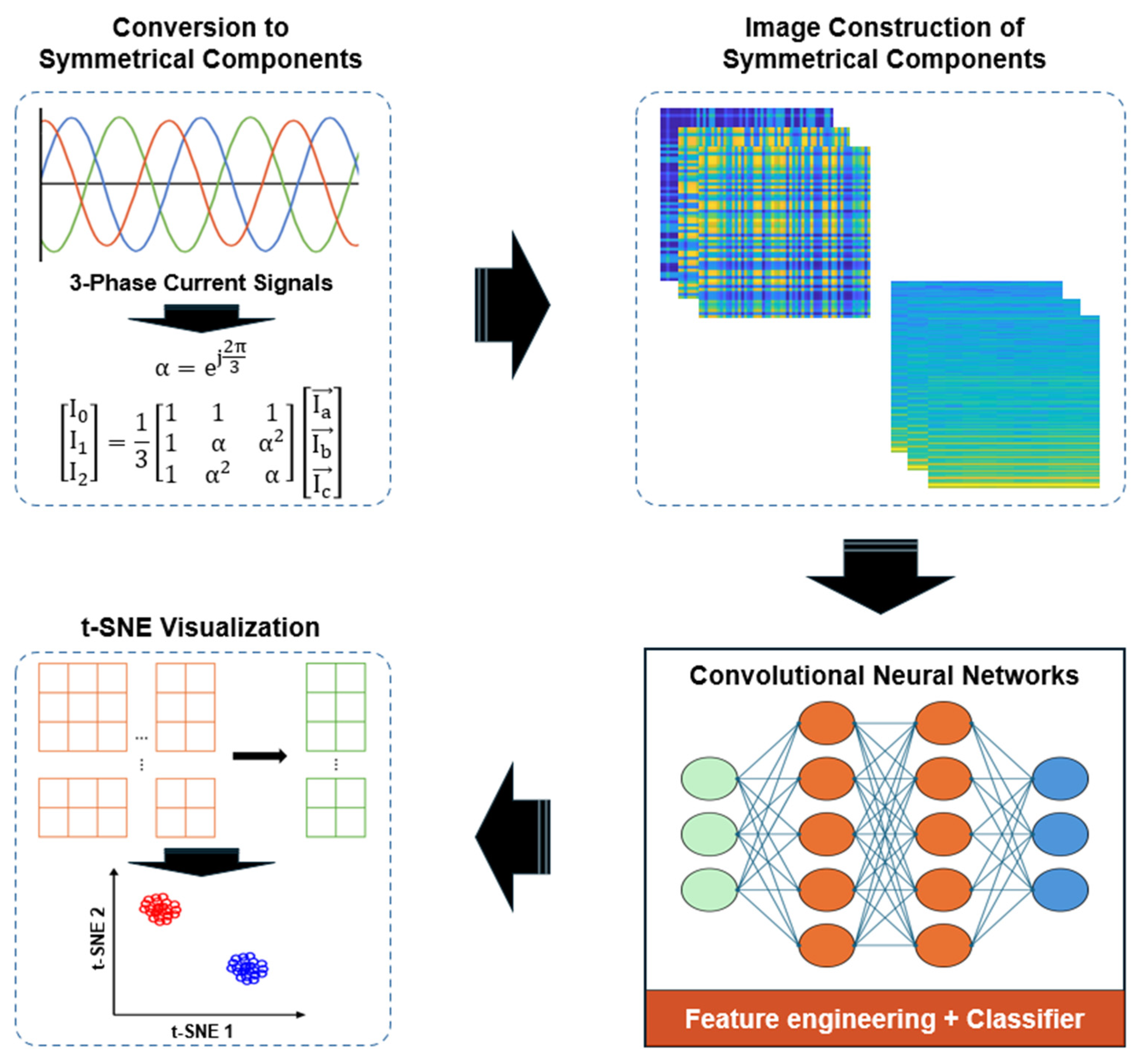
Figure 1. Flowchart of the overall methodology introduced in this paper.
Electronics 14 01679 g001
Figure 2. Conversion of three-phase stator currents to symmetrical components (zero, positive, and negative sequences).
Electronics 14 01679 g002
Figure 3. Image construction using feature vectors of symmetrical components.
Electronics 14 01679 g003
Figure 4. Experimental setup for data acquisition. (a) Schematic of the motor test system. (b) Photo of the rotor kit.
Electronics 14 01679 g004
Figure 5. Simulating faults in the experimental model. (a) Bowed shaft. (b) Unbalance. (c) Broken rotor bar. (d) Single phasing and voltage unbalance. (e) Stator winding fault.
Electronics 14 01679 g005
Figure 6. Time waveform of symmetrical components in seven different conditions: (a) Normal; (b) Bowed shaft; (c) Unbalance; (d) Broken rotor bar; (e) Single phasing; (f) Voltage unbalance; (g) Stator winding fault.
Electronics 14 01679 g006
Figure 7. RMS values of symmetrical components. (a) RMS of zero sequence. (b) RMS of positive sequence. (c) RMS of negative sequence.
Electronics 14 01679 g007
Figure 8. Example of CNN model architecture.
Electronics 14 01679 g008
Figure 9. Architecture of CNN model for training.
Electronics 14 01679 g009
Figure 10. Confusion matrices for the seven-class classification problem. (a) STFT-based method. (b) Proposed symmetrical components-based method.
Electronics 14 01679 g010
Figure 11. t-SNE plots of high-dimensional features (projected to 2D) learned by the CNNs. (a) Features from the STFT spectrogram CNN. (b) Features from the proposed symmetrical component image CNN.
Electronics 14 01679 g011
Figure 12. Sample comparison of visual patterns from the two methods for all seven conditions. (a) STFT-based spectrogram image. (b) Proposed symmetrical components feature image.
Electronics 14 01679 g012
Table 1. Definition of the nineteen time-domain feature parameters.
FeaturesDefinition (Equation)
Peak f 1 = max x
RMS f 2 = 1 N n = 1 N x n 2
Kurtosis f 3 = 1 N n = 1 N x n x ¯ σ 4
Crest factor f 4 = max x n 1 N n = 1 N x n 2
Clearance factor f 5 = max x 1 N n = 1 N x n 2
Impulse factor f 6 = max x 1 N n = 1 N x n
Shape factor f 7 = 1 N n = 1 N x n 2 1 N n = 1 N x n
Skewness f 8 = 1 N n = 1 N x n x ¯ σ 3
Square mean root f 9 = 1 N n = 1 N x n 2
5th normalized moment f 10 = 1 N n = 1 N x n x ¯ σ 5
6th normalized moment f 11 = 1 N n = 1 N x n x ¯ σ 6
Mean f 12 = 1 N n = 1 N x n
Shape factor 2 f 13 = 1 N n = 1 N x n 2 1 N n = 1 N x n
Peak to peak f 14 = max x min x
Kurtosis factor f 15 = 1 N n = 1 N x n x ¯ σ 4 1 N n = 1 N x n 2 2
Standard deviation f 16 = 1 N n = 1 N x n x 2
Smoothness f 17 = 1 ( 1 + 1 N n = 1 N x n x 2 2
Uniformity f 18 = 1 1 N n = 1 N x n x 2 1 N n = 1 N x n
Normal negative log-likelihood f 19 = 1 σ 2 π e x μ 2 2 σ 2
Table 2. Data acquisition system properties (current sensors and DAQ).
TypeProperties
Pulse 3560c
(B&K)
  • 5/1-ch Input/output collector module
  • Operating frequency range: 0~25.6 kHz
  • Direct/constant current line drive (CCLD)/Microphone (MIC), preamp 1 tacho
AC Current Clamp
(FLUKE i200s)
  • Measuring range: 0.1~24 A
  • Operating temperature: −10~55 °C
  • Sensitivity: 10 mV/A
Table 3. Data acquisition settings for experiments.
ConditionValue
Operating speed20 Hz (constant)
Sampling rate65,536 Hz
Recording duration60 s per experiment
Table 4. Classes of simulated motor conditions (fault induction summary).
No.ConditionFault Type
1Normal(Baseline)
2Bowed shaftMechanical fault
3Unbalance
4Broken rotor barElectrical fault
5Single phasing
6Voltage unbalance
7Stator winding fault
Table 5. RMS values symmetrical components.
Division1234567
Zero-sequence of RMS0.0350.0350.0340.0340.0250.0330.033
Positive-sequence of RMS1.261.241.241.231.011.081.25
Negative-sequence of RMS0.030.030.020.031.000.620.09
Disclaimer/Publisher’s Note: The statements, opinions and data contained in all publications are solely those of the individual author(s) and contributor(s) and not of MDPI and/or the editor(s). MDPI and/or the editor(s) disclaim responsibility for any injury to people or property resulting from any ideas, methods, instructions or products referred to in the content.