Abstract
At present, the detection of steel surface defects is still challenging, because there are some problems in steel products, such as complex background and noise interference, making it difficult to accurately detect complex small targets and great changes in defects at different scales, which directly affects product quality and endangers life safety. To solve the above problems, this paper proposes a steel surface defect detection network based on global attention perception and cross-layer interactive fusion, named GCF-Net. Firstly, this paper proposes an Interactive Feature Extraction Network (IFE-Net), which uses a local modeling feature extraction module to enhance the extraction of local detail features and uses a global attention perception module to capture the global contextual information in the image, thus improving the detection of complex background and noise defects. Secondly, this paper proposes a Cross-Layer Interactive Fusion Network (CIF-Net), which makes up for the fine-grained information lost during the gradual refinement of features through the fusion of adjacent layers, fully integrates shallow and deep features, and at the same time enhances the interaction between different scales by cross-layer fusion, thus improving the recognition ability of defect targets of different scales. Thirdly, the Interactive Fusion Module (IFM) is proposed, which can adjust the importance of each mosaic feature by attention to make efficient use of all feature information and improve the detection of complex background defects. Finally, in order to solve the problems of difficult positioning and inaccurate detection of small targets, this paper aims to strengthen the sensitive loss Q_IOU of small targets and improve the perception of complex small targets in steel defects. Compared with the baseline model, mAP@.5 is improved by 7.0%, 4.4%, and 2.5% on the NEU-DET, PCB, and Steel datasets, respectively, and it is better than all of the comparison models.
1. Introduction
Surface defect detection of industrial products [1] is a key link to ensure the quality and safety of products, which involves using advanced technology to identify and classify the surface defects of products [2], such as cracks and scratches, which not only affect the beauty of the products but also may reduce their durability and performance. Therefore, steel surface defect detection has become one of the main tasks for metallurgical enterprises to improve steel quality. Traditional inspection methods, such as manual inspection, nondestructive inspection, and laser scanning inspection [3], are time-consuming, inefficient, inaccurate, and struggle to classify defects.
In the detection of surface defects on metal products [4], one-stage detection methods, exemplified by the YOLO [5] series and SSD [6] algorithms, predict the class and bounding boxes of objects directly, offering relatively lower performance. Two-stage detection, represented by FAST R-CNN [7] and Mask R-CNN [8], generates candidate regions through a Regional Proposal Network (RPN), and then it classifies these regions and regresses the bounding box.
For example, Tang et al. [9] systematically analyzed steel surface defect detection methods, which brought a new perspective to studying steel defect detection based on deep learning. Cui et al. [10] proposed a fast and accurate surface defect detection network, designed a jump connection module, and propagated fine-grained features to improve defect detection accuracy. Li et al. [11] put forward a steel surface defect detection model based on the YOLO algorithm, designed a novel attention-embedding backbone network to improve the attention to defect features, and improved the perception ability of defect features. Gao et al. [12] proposed a transformer structure for surface defect detection, designing a hybrid backbone network. Although it improved the defect detection, the huge parameters that it brought were also worthy of our attention. You et al. [13] used cross-attention to calculate the weight of each channel, which helped extract specific feature areas, design semantic perception modules, enhance deep defect feature extraction, and further improve defect detection. Du et al. [14] designed a feature extraction network by using Mobile Inverted Residual Bottleneck Block to enhance the perception of PCB surface defects. However, the detection of surface defects on industrial products still faces multiple challenges, and at the same time, it is necessary to accurately identify various defects and show strong adaptability and stability.
Although the above-mentioned detection method based on deep learning has achieved certain advantages, it faces many challenges in steel defect detection: (1) Complexity of defect background: It is difficult for a general detector to capture the global context information in an image, which makes it difficult to accurately detect complex background information. (2) Small target defect detection: The semantic information of small target defects is weak, which makes it difficult to detect and locate the loss function accurately. (3) Multi-scale defects: The scale of the detected object changes dramatically, which makes it difficult for the feature fusion network to fully capture the characteristics of deep and shallow defects, resulting in poor detection results. In fact, more attention should be paid to the extraction of local and global contextual information in the process of steel defect detection, and at the same time, the accurate identification of defects with weak semantic information and the effective detection of defects with significant scale changes should be improved.
In view of this problem, this study introduces a detection network for steel surface defects that leverages global attention perception and cross-layer interaction fusion (GCF-Net), aiming to improve the identification and location of steel surface defects in industrial scenes. To address the identified issues, this paper initially develops an Interactive Feature Extraction Network (IFE-Net) that incorporates both a local modeling feature extraction module and a global attention perception module. Secondly, a Cross-Layer Interactive Fusion Network (CIF-Net) is proposed to improve the recognition and location of targets. The Interactive Fusion Module (IFM) is proposed, which uses the dynamic feature selection process to adjust the importance of each mosaic feature through attention, to make efficient use of each feature’s information.
The main contributions of this method are as follows:
- (1)
- In this paper, an IFE-Net is designed to improve the extraction of local detail features. The local modeling feature extraction module (LMF) is designed to fully extract the local details of steel surface defects, and the local feature extraction module (LS Block) is used to enhance the local feature extraction, while the residual feature extraction module (RG Block) is used to retain and utilize the spatial structure information of the image, so as to improve the defect detection performance. In addition, the Global Attention Interaction Module (AIM) is introduced to capture the global contextual information in the image, so as to improve the detection ability of the model for defects under various background noises and interferences.
- (2)
- Aiming at the problem of low detection accuracy caused by the large changes in defect size, this paper proposes a CIF-Net. By merging the features of adjacent layers, the network supplements the lost detailed information in the process of feature refinement, giving full play to the advantages of detailed features and deep semantic information. Finally, the interaction between different-sized features is strengthened by cross-layer fusion technology.
- (3)
- To comprehensively adjust the importance of each feature in the mosaic, an IFM is proposed, which uses the dynamic feature selection process and adjusts the features to be fused from the perspectives of channel and space to improve the recognition of complex background defects.
- (4)
- To meet the challenge of low detection accuracy of small targets, an enhanced small target sensitivity loss Q_IOU is designed in this study, aiming at improving the model’s ability to identify complex small defects on steel surfaces.
The rest of this paper is organized as follows: Section 2 introduces the literature review of related work, focusing on the analysis of defect detection networks based on deep learning. Section 3 introduces the method proposed in this paper and the function of each module in detail. Section 4 introduces the experiment and analysis of this paper, including ablation and contrast experiments. Section 5 presents the discussion. Section 6 provides the conclusions and future prospects.
2. Related Work
2.1. Surface Defect Detection
The evolution of surface defect detection [15] has transitioned from conventional image processing techniques to contemporary approaches that leverage deep learning [16]. Historically, detection methods have been predicated on manually crafted feature extraction, including practices like edge detection [17] and texture analysis. These methods have high requirements for the imaging environment, poor adaptability, and are greatly influenced by subjective factors.
As deep learning technology has advanced, CNN-based detection methods [18] have gained prominence due to their robust feature learning capabilities. These methods are capable of autonomously extracting features from extensive datasets, offering enhanced flexibility and precision. Within industrial applications, a variety of sophisticated detection techniques have arisen, alongside the broad utilization of deep learning for object detection. Broadly, these detection technologies fall into two categories:
The first category encompasses one-stage detection approaches, including models like YOLO, SSD, and RetinaNet [19], which directly predict the positions of categories and bounding boxes in the network at the same time, without generating the candidate areas separately. However, due to the omission of the generation process of candidate regions, one-stage detection methods [20] may be slightly inferior in positioning and classification. The other category is two-stage detection methods, such as the R-CNN series [21]. First, candidate frames that may contain defects are generated through the Regional Proposal Network (RPN), and then the target is further detected. This method usually performs better in accuracy because it can extract the region of interest carefully, thus reducing the false recognition rate and missed recognition rate. However, due to the need for two-stage calculation, two-stage detection methods [22] are slow in processing speed and suitable for scenes with high detection accuracy.
For example, Xiao et al. [23] developed an attention mechanism module, which can encode average features and salient features in two spatial dimensions, to capture the spatial correlation in images. Yang [24] and others put forward a lightweight surface defect detection method and added an attention module. Li et al. [25] adopted channel attention and pixel attention at the same time, which made the network learn more robust features, learn defect feature distribution, and improve defect detection accuracy. Song et al. [26] used deep semantic information to guide shallow features to improve the detection.
Unlike past approaches, this paper proposes a steel surface defect detection network, designs an IFE-Net, enhances the extraction of local detail features, and captures the global contextual information in the image, thus improving the model’s detection of defects with different backgrounds and noise interference. Secondly, a CIF-Net is designed to improve the detection accuracy. Finally, the IFM is proposed, which uses the dynamic feature selection process to adjust the importance of each splicing feature by paying attention to make efficient use of all feature information.
2.2. Multi-Scale Feature Fusion Network
A fusion network [27] is a deep learning architecture, integrating feature information from different levels. It uses a feature pyramid structure to combine high-level semantic features with low-level detail features through upsampling and downsampling operations [28]. The network also includes parallel multi-branch networks, such as the Inception [29] network, for pooling operations. A serial layer-hopping connection structure, such as the skip-connection structure in the U-Net [30] network, fuses shallow features with deep features by introducing short connections into the network [31]. A variety of networks have emerged, such as FPN [32], PANet [33], BiFPN [34], etc. Although these networks have achieved remarkable results in multi-scale feature fusion, they cannot efficiently fuse the multi-layer features extracted from the backbone network.
In response to the aforementioned challenges, this study introduces an IFE-Net that spans across layers. By integrating features from neighboring layers, this network compensates for the fine details. Cross-layer fusion is used to enhance the interaction between different scales and improve the recognition ability of targets at different scales.
3. Method
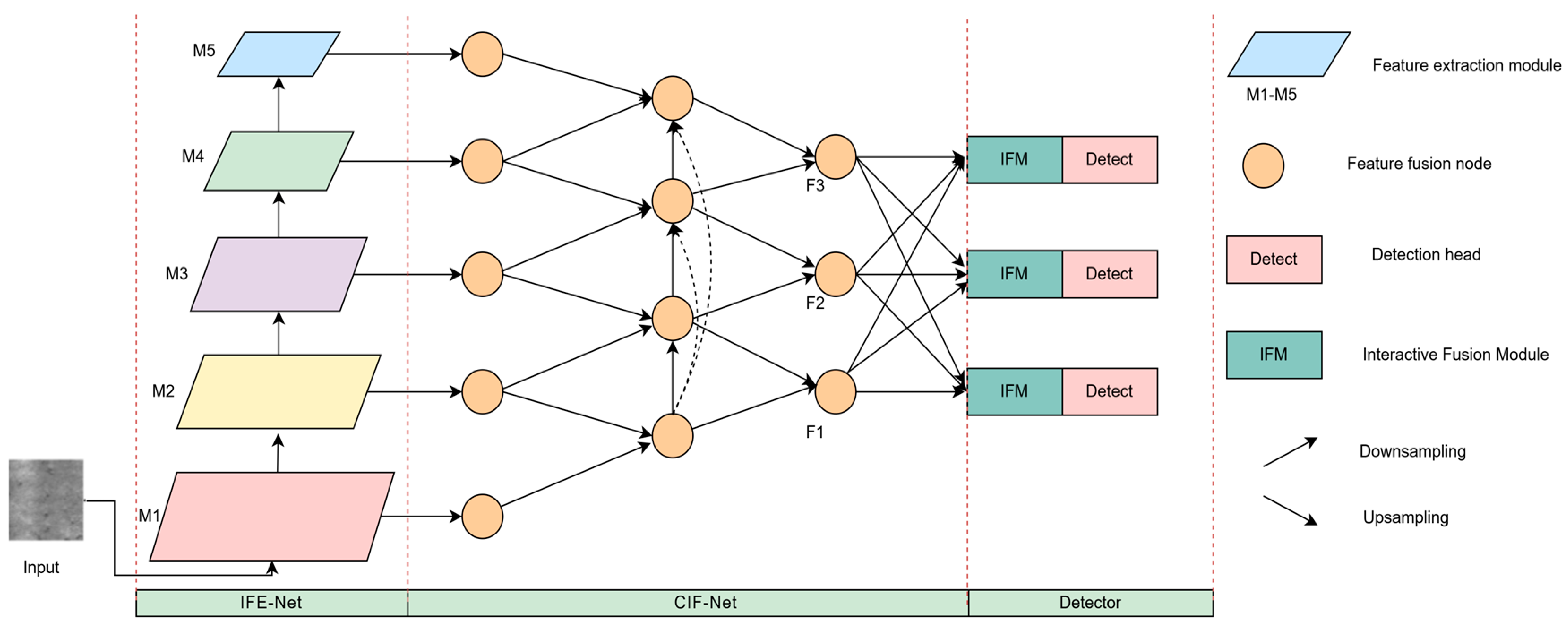
As shown in Figure 1, the GCF-Net network structure proposed in this paper consists of an Interactive Feature Extraction Network (IFE-Net), Cross-Layer Interactive Fusion Network (CIF-Net), Interactive Fusion Module (IFM), and three detectors with different sizes. Firstly, the local and global contextual defect features are fully extracted from the input feature map through the IFE-Net. The IFE-Net consists of five feature extraction modules, and each layer downsamples the input feature map twice as much as the original one. Secondly, the features at all levels extracted from the IFE-Net pass through the CIF-Net, and the fine-grained information lost during the gradual refinement of features is compensated by the fusion of adjacent layers, so as to improve the recognition ability of targets at different scales. Then, the output of the CIF-Net is input to the IFM, and the dynamic feature selection process is used to adjust the features to be fused from the perspectives of channel and space, so as to improve the recognition of complex background defects. Finally, the features fused by the IFM are input into three detection heads with different sizes to enhance the attention of the network to the key areas around the target object and output the defect detection results.

Figure 1.
GCF-Net overall structure diagram.
The IFE-Net constructed in this paper is shown in Figure 2. M1 is composed of a convolution unit, and M2–M4 are composed of a convolution unit and a local modeling feature extraction module (LMF). The LMF module fully extracts the local details of steel surface defects, and the local feature extraction module (LS Block) is used to enhance the local feature extraction, while the residual feature extraction module (RG Block) is used to retain and utilize the spatial structure information of the image. M5 is a Global Attention Interaction Module (AIM) designed in this paper. The local features extracted by the LMF module are input into the AIM at the end of the network, and then the global contextual information of the image is captured. The features in different channel groups are deeply fused by point-by-point convolution, so as to realize information interaction and feature enhancement between channels and improve the detection ability of the model under various background noises and interferences.
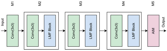
Figure 2.
Structure diagram of IFE-Net.
3.1. Local Modeling Feature Extraction Module
In an effort to thoroughly capture the local characteristics of the steel surface defects, and to more precisely detect and differentiate between various types of defects, this study introduces a local modeling feature extraction module (LMF), as illustrated in Figure 3. A local feature extraction module (LS Block) is used to enhance the extraction of local features. Because standard convolution often adopts cross-channel information mixing when extracting features, it cannot effectively extract local information between different channels, and at the same time it brings a large amount of parameters. Therefore, for a given input feature, it first carries out depth-separable convolution, which effectively extracts the local spatial information of the input feature map for each input channel without mixing the channel information, while reducing the calculation cost and the number of parameters, and then carries out batch normalization, and finally adjusts the number of channels through 1 × 1 convolution to extract fine-grained features.
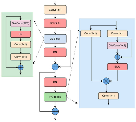
Figure 3.
Local modeling feature extraction module; BN is the batch normalization layer, DWConv is the depthwise convolution module, and SiLU is the activation function.
To prevent the gradient degeneration in deep neural networks and enhance the reusability and expressive ability of the features, this paper uses the residual feature extraction module (RG Block) to retain and utilize the spatial structural information of images and reuse the input features. Specifically, first, the channels are mixed through a 1 × 1 convolution layer, and then one branch continues to pass through another 1 × 1 convolution layer, followed by a 3 × 3 depth-separable convolution to extract spatial features. Finally, the characteristic channels are further mixed through a 1 × 1 convolution layer. The design of the whole module aims to reduce the calculation cost and return the gradient more effectively through residual connection, and the calculation cost is lower, while retaining and utilizing the spatial structural information of the image, thus improving the performance of the model. The RG Block can be expressed by Formulae (1) and (2):
where F is the input characteristic diagram, F′ is the output characteristic of the residual differential branch in the right half of the RG Block module, and F″ is the output characteristic of the RG Block module.
3.2. Global Attention Interaction Module
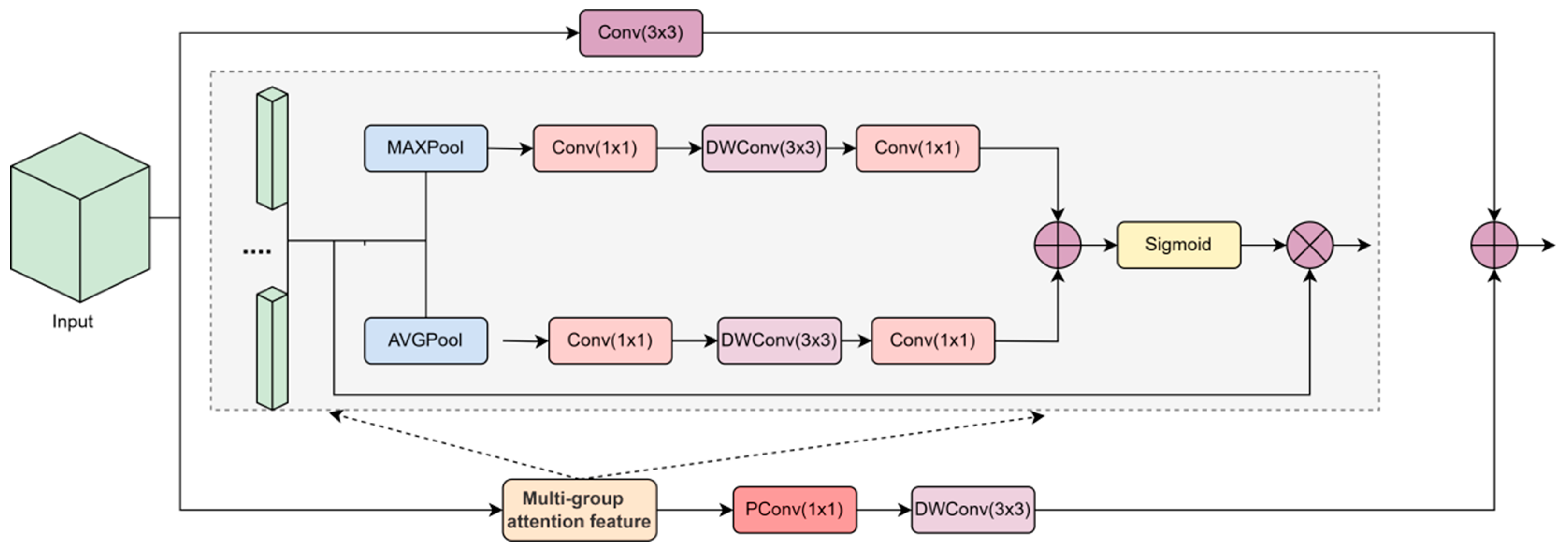
To make the network pay attention to the local detail texture in global features and solve the problem of inaccurate defect classification caused by weak semantic information of the steel surface, this paper designs a Global Attention Interaction Module, (AIM) to enhance the semantic information of defect surface features, as shown in Figure 4. The module is composed of two distinct pathways: a multi-branch attention mechanism, and a 3 × 3 convolution process. Initially, the incoming feature map is partitioned into n channels using group convolution. Afterwards, an adaptive pooling layer sequentially consolidates the feature map across channels. Subsequently, these aggregated features are transferred to the depth-separable convolution layer, which is responsible for compressing the spatial dimensions of the feature map. The generated attention score is multiplied with the original feature map to highlight the key information in each channel group. Finally, the features in the channel group are deeply fused by point-by-point convolution to realize information interaction and feature enhancement between channels. This process not only enhances the ability of feature representation but also gives the model fine-grained control over different channel features through the attention mechanism.
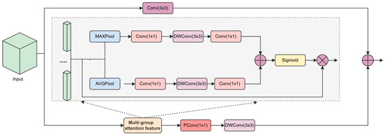
Figure 4.
Global Attention Interaction Module.
This process can be expressed by Formulae (3) to (7).
Firstly, the input features f are divided into m groups by block convolution:
where F1 is the feature after adaptive maximum pooling and depthwise convolution, F2 is the feature after adaptive average pooling and depthwise convolution, and F3 is the feature after fusing F1 and F2.
Then, the obtained groups of attention features are subjected to point-by-point convolution of 1 × 1 and depth-separable convolution of 3 × 3, and the features in the channel groups are deeply fused to realize information interaction and feature enhancement between channels.
F4 is the feature after multi-branch attention operation and depthwise convolution.
Finally, the features of the two branches are fused to realize the intra-block feature aggregation between different dimensions and improve the characterization of fine-grained defect features.
3.3. Cross-Layer Interactive Fusion Network
Figure 5 shows the different common feature fusion networks, among which FPN loses detailed information in the process of feature fusion. PANet adds a bottom–up feature transfer path, but the parameters are too large and the efficiency is not high. BiFPN is insufficient in integrating the spatial features captured from different levels of the backbone network.
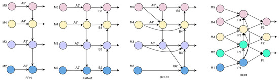
Figure 5.
Comparison of several different feature fusion networks.
To solve these problems, this paper proposes a Cross-Layer Interactive Fusion Network (CIF-Net). Specifically, unlike the past approaches, PConv convolution is used to replace ordinary convolution, and the fusion method is reduced layer by layer to reduce the model parameters. Secondly, the loss of detailed information due to the progressive feature refinement is mitigated through the integration of nearby layers. Finally, the integration process, by focusing excessively on the transfer and aggregation among adjacent feature layers, overlooks the progressive interaction between features across different layers, and it uses cross-layer fusion to enhance the interaction between different scales. This allows the network to concurrently take into account both the fine details and the broader context of the image, thereby enhancing its capacity to recognize targets across a range of scales.
The comparison between the fusion network proposed in this paper and FPN, PANet, and BiFPN is shown in Figure 5. For example, P3 in the figure can be expressed by Formulae (8) to (10):
where represents two times of downsampling, represents four times of downsampling, and represents the splicing operation of different feature maps, where is a very small positive number to prevent unstable training, and represents the weight coefficient that can be learned. P3, P2, and P1 are new feature layers after cross-layer feature fusion.
3.4. Interactive Fusion Module
In the existing methods of fusing features of the same size, the features are often fused in an undifferentiated way. However, this kind of fusion method, regardless of priority, can easily lead to the loss of important information and the interference of useless information. In this section, an IFM is designed, which can adjust the importance of each mosaic feature by attention to making efficient use of all feature information, and then embed it into the enhanced feature pyramid network to improve the detection of defects in complex backgrounds.
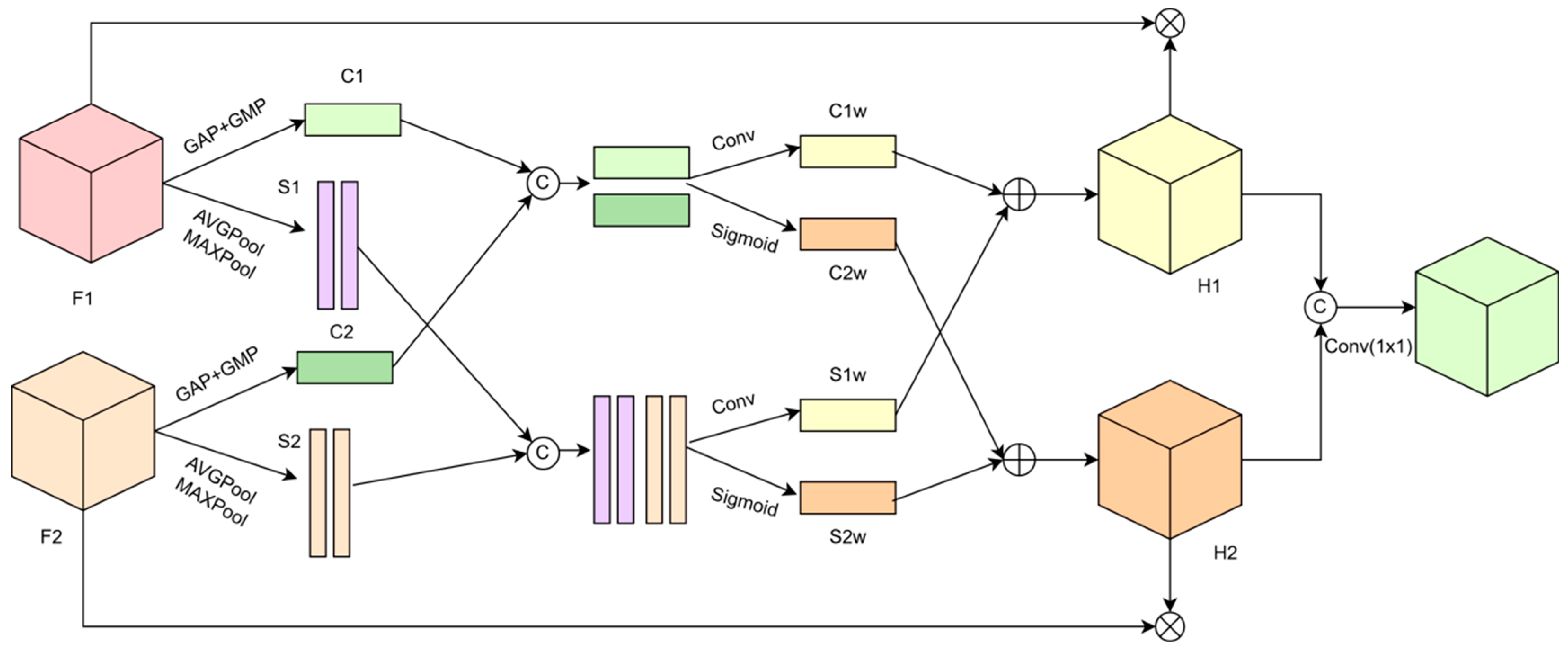
To comprehensively adjust the importance of each feature in stitching, the IFM simultaneously adjusts the features to be stitched from the perspectives of channel and space. In Figure 6, the Interactive Fusion Module (IFM)’s architecture is illustrated with a simplified representation of two input features for clarity. The module accepts features F1 and F2 to be concatenated. It initiates the process by employing global average pooling (GAP) and global maximum pooling (GMP) to extract global features from each, subsequently summing these extracted features.
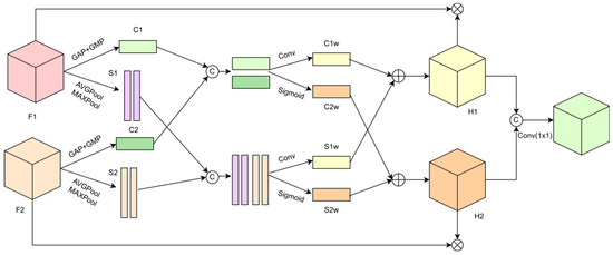
Figure 6.
Interactive Fusion Module.
This process can be represented by Equations (11) and (12):
where GAP is the global average pooling, GMP is the global maximum pooling, and + is an element-by-element addition operation.
The spatial features obtained from their respective features are spliced in the channel direction. This process can be represented by Equations (13) and (14):
where Concat stands for splicing, AVGPool stands for average pooling, and MAXPool stands for maximum pooling.
To comprehensively consider the stitching features to evaluate their importance, the IFM fuses the channel and spatial features obtained from the input features F1 and F2, respectively, and then it comprehensively uses this information to adjust the values of the elements of the input features F1 and F2. The channel features are spliced, the spliced comprehensive features are input into two 1 × 1 convolution layers, and the input results are converted into adjustable weights by using the sigmoid function. This process can be expressed by Equation (15):
where represents 1 × 1 convolution, Cat represents the splicing operation, and sigmoid is the activation function.
Similarly, the spatial features are spliced in the channel direction, the spliced features are input into two 1 × 1 convolutions, and the sigmoid function is used to convert them into adjustment values. This process can be expressed by Equation (16):
After the number of channels is adjusted by 1 × 1 convolution, this process can be expressed by Equation (17):
3.5. Loss Function
The loss function [35] in one-stage target detection consists of classification loss, confidence loss, and prediction frame regression loss. The Binary Cross-Entropy (BCE) loss [36] is utilized for determining both the confidence and classification losses, whereas the bounding-box regression loss is determined by the CIoU loss [37]. The CIoU loss incorporates factors such as the intersection over union, the distance between the centers of the predicted and actual bounding boxes, and the aspect ratio. Typically, when the CIoU loss value is high, it indicates a greater discrepancy in the central point positioning between the predicted and actual bounding frames, so the loss for larger targets will be considerably greater than for smaller targets during the loss computation process, which negatively impacts the loss calculation for smaller targets, resulting in the inaccuracy of the model in detecting the small targets in surface defects. Hence, in light of the challenges associated with pinpointing small targets, this study refines the penalty term to enhance the sensitivity of the Q_IOU loss specifically for minor targets, which is used to improve the perception of complex small targets in steel defects. Q_IOU can be expressed by Formulae (18) to (20):
where IoU is calculated as the proportion of the overlapping area between the predicted and actual bounding boxes to their combined area; represents the Euclidean distance between the center points of the prediction frame and the rear frame; b and are the center points of the prediction frame and the real frame, respectively; and are the width and height of the real frame, respectively; and w and h are the width and height of the prediction frame, respectively.
4. Experiment and Analysis
4.1. Experimental Parameters
The configuration used in the experiment included a Windows 11 system and NVIDIA GeForce RTX 3080 24 GB graphics card, and the compilation environment was PyTorch 1.11.1, Python 3.8, and CUDA 11.3. The image input size was set to 640 × 640, the batch size was set to 32, and the number of training rounds (epochs) was set to 300.
4.2. Evaluation Indicators
For the purpose of assessing the model’s effectiveness in an impartial manner, this study employs precision (P), recall (R), and mean average precision (mAP) as the key metrics, which are widely recognized standards within the domain of object detection for evaluating performance.
From this, the formulae for accuracy and recall can be obtained as Equations (21) and (22), respectively:
where Indicates that the test sample is divided into positive samples and the classification is correct, signifies that the samples identified as positive are incorrectly labeled, and denotes the count of positive samples that have been falsely predicted.
The mean average precision mAP can be expressed as shown in Equation (23):
where C is a different kind of defect.
F1 is expressed as shown in Equation (24):
4.3. NEU-DET Dataset Experiment
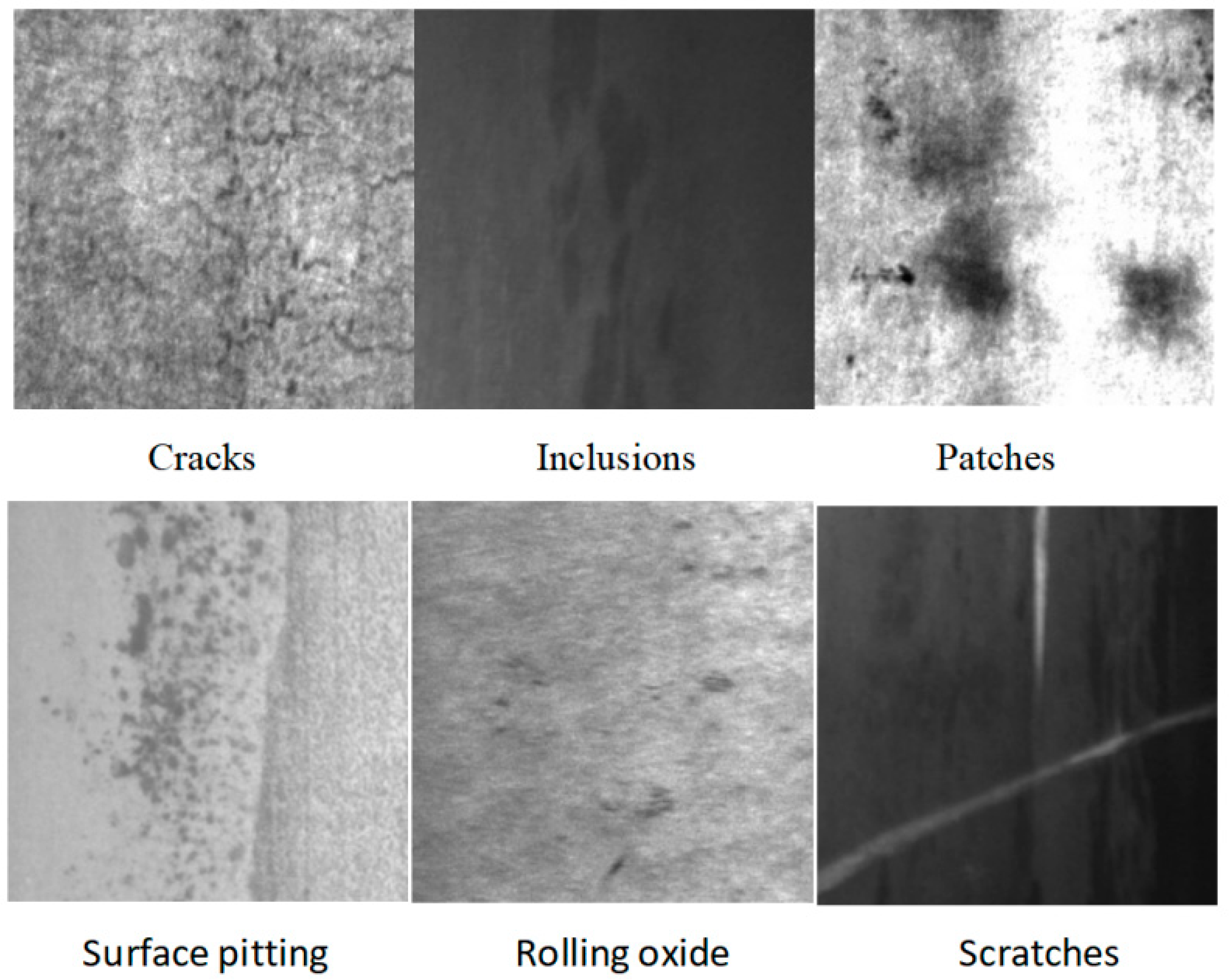
In this paper, the NEU-DET [38] steel dataset published by Northeastern University was used for experiments. There are six kinds of defects in this dataset: cracks (Cr), inclusions (ln), patches (Pa), pits (Ps), scars (Rs), and scratches (SC), with 300 pictures of each kind of defect, for a total of 1800. To enhance the robustness and generalization of the model, 1800 pictures in the dataset were rotated, supplemented with noise, flipped, and changed in brightness to broaden the dataset. Ultimately, a novel dataset comprising 3600 samples was compiled. For this study, the dataset was randomly partitioned into training and testing subsets, at a proportion of 9:1. The experiment was carried out utilizing publicly available datasets, which can compare the performance of the model and are more extensive. Part of the steel dataset is shown in Figure 7.
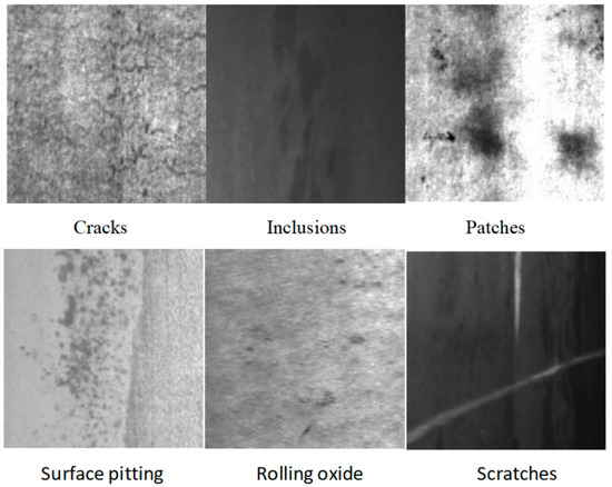
Figure 7.
Six types of defects in the steel dataset.
4.3.1. Ablation Research of Different Modules
The experimental results are shown in Table 1. As can be seen from the following table, showing the second behavior of the ablation experiment for the interactive backbone feature extraction network proposed in this paper on the baseline model, the R-value increased by 4.9%, and the mAP@.5 value increased by 5.5%, due to the IFE-Net being designed to seize both the intricate local features and the overarching contextual details present within the image, thus improving the model’s detection of different backgrounds and noise interference defects. The third line is the ablation research of CIF-Net, a Cross-Layer Interactive Fusion Network.

Table 1.
Ablation experiment on the NEU-DET steel dataset.
Compared with the baseline model, the R-value increased by 4.4%, and the mAP@.5 value increased by 4.6%. When adding the efficient fusion module IFM, adjusting the features to be fused from the perspectives of channel and space, and with attention to making efficient use of all feature information, the value of mAP@.5 increased by 1.8%. Q_IOU was designed to strengthen the sensitive loss of small targets and improve the perception of complex small targets in steel defects, and the mAP@.5 value increased by 1.0%. In addition, FPS represents the number of image frames processed per second during the model training.
4.3.2. Ablation Experiment
Table 2 shows the influence of different modules of the backbone network. With the addition of the local modeling feature extraction module (LMF Block), the R-value increased by 1.9% and the mAP@.5 value increased by 1.7%, due to the enhancement of the local feature extraction by the local feature extraction module (LS Block). The RG Block, a component for residual feature extraction, plays a crucial role in preserving and leveraging the spatial configuration of images, thereby substantially enhancing the system’s effectiveness. By adding the Global Attention Interaction Module (AIM), the network can pay attention to the local details and textures in the global features, solve the problem of inaccurate defect classification caused by weak semantic information of the steel surface, and enhance the semantic information of the defect surface. Compared with the baseline model, the R-value increased by 4.1%, and the mAP@.5 value increased by 4.8%.
Table 2.
Influence of different modules.
Figure 8 shows the thermal map of the YOLOv5s model and the addition of the AIM under the interference of steel noise. The addition of the AIM highlights local key feature areas, and the features’ texture is more obvious, thus improving the ability of defect location and identification.
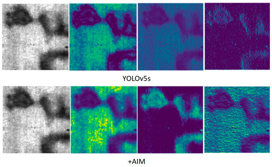
Figure 8.
Thermal diagram of AIM under noise interference.
4.3.3. Comparative Test in NEU-DET Dataset
Table 3 shows the comparison between the GCF-Net model in this paper and other mainstream target detection models on the steel dataset, including the one-stage and the two-stage detection models. As can be seen from the following table, GCF-Net obtained the highest mAP value, and the R value was slightly lower than that of the Faster R-CNN model, but the parameters and detection speed of this model were far superior to those of Faster R-CNN. On the whole, this model showed the best performance. Compared with the models YOLOX, YOLOv7s, PP-YOLOE, and YOLOR, which have little difference in their parameters, the R-value increased by 2.2%, 6.0%, 0.2%, and 5.3% respectively, and the mAP value increased by 3.0%, 7.3%, 0.4%, and 6.2% respectively.
Table 3.
Comparative experiments of different models in NEU-DET datasets.
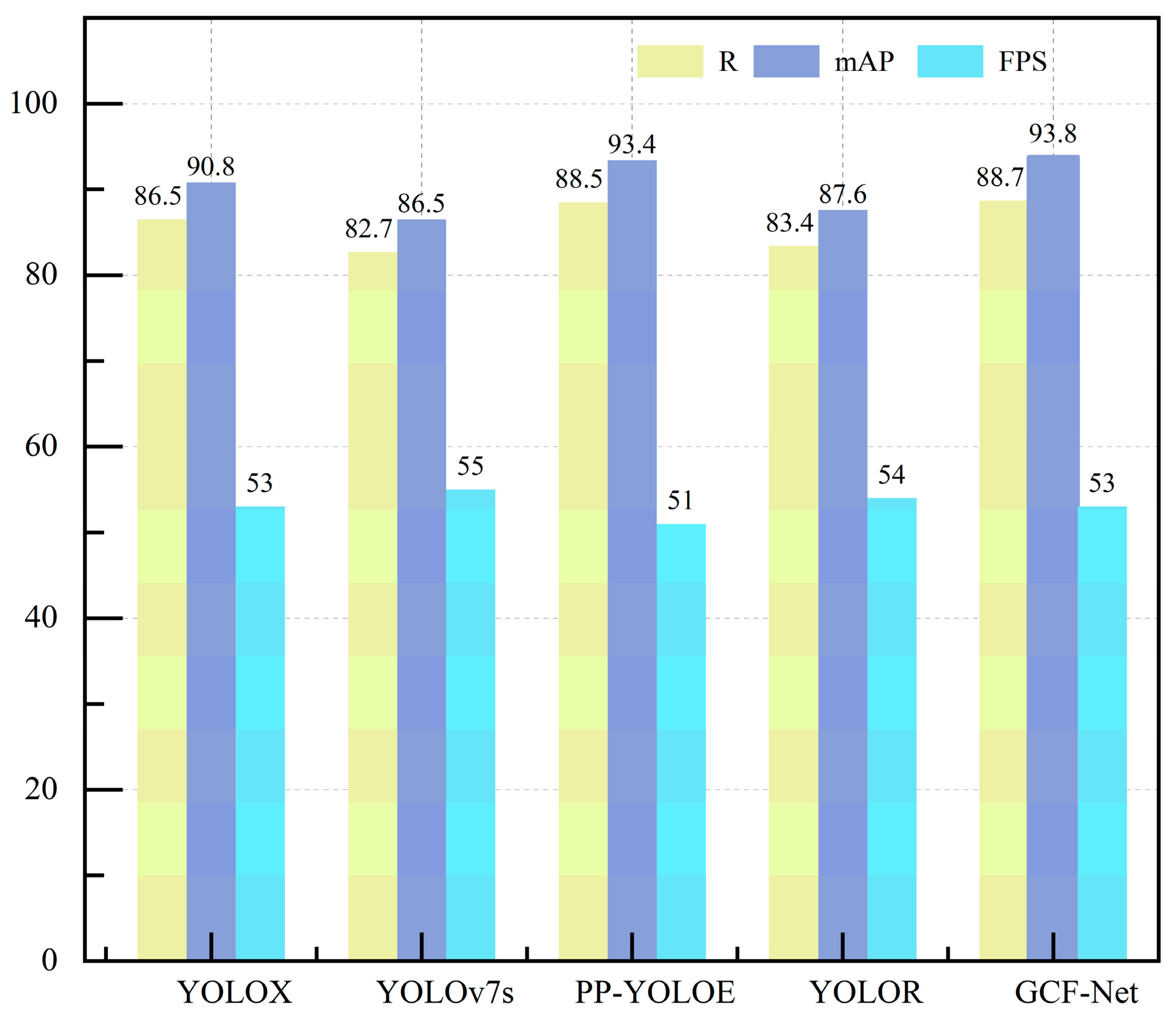
Therefore, it can be seen that the ability of GCF-Net to detect steel surface defects is more significant than that of other models. CIF-Net is used to compensate for the loss of detailed information that occurs as features are progressively reduced by combining layers that are in close proximity, and the multi-scale defect detection of the steel surface is improved. Figure 9 shows the detection results of this model and the YOLOX, YOLOv7s, PP-YOLOE, and YOLOR models on R, mAP, FPS, and other indicators. It can be seen that this model obtained the highest mAP value, and the detection speed was slightly lower than that of YOLOv7s. Considering all of the indicators fully shows that this method can accurately identify steel surface defects.
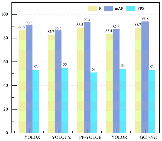
Figure 9.
Comparison of R, mAP and FPS of different models in NEU-DET datasets.
4.3.4. Visualization Research in NEU-DET Datasets
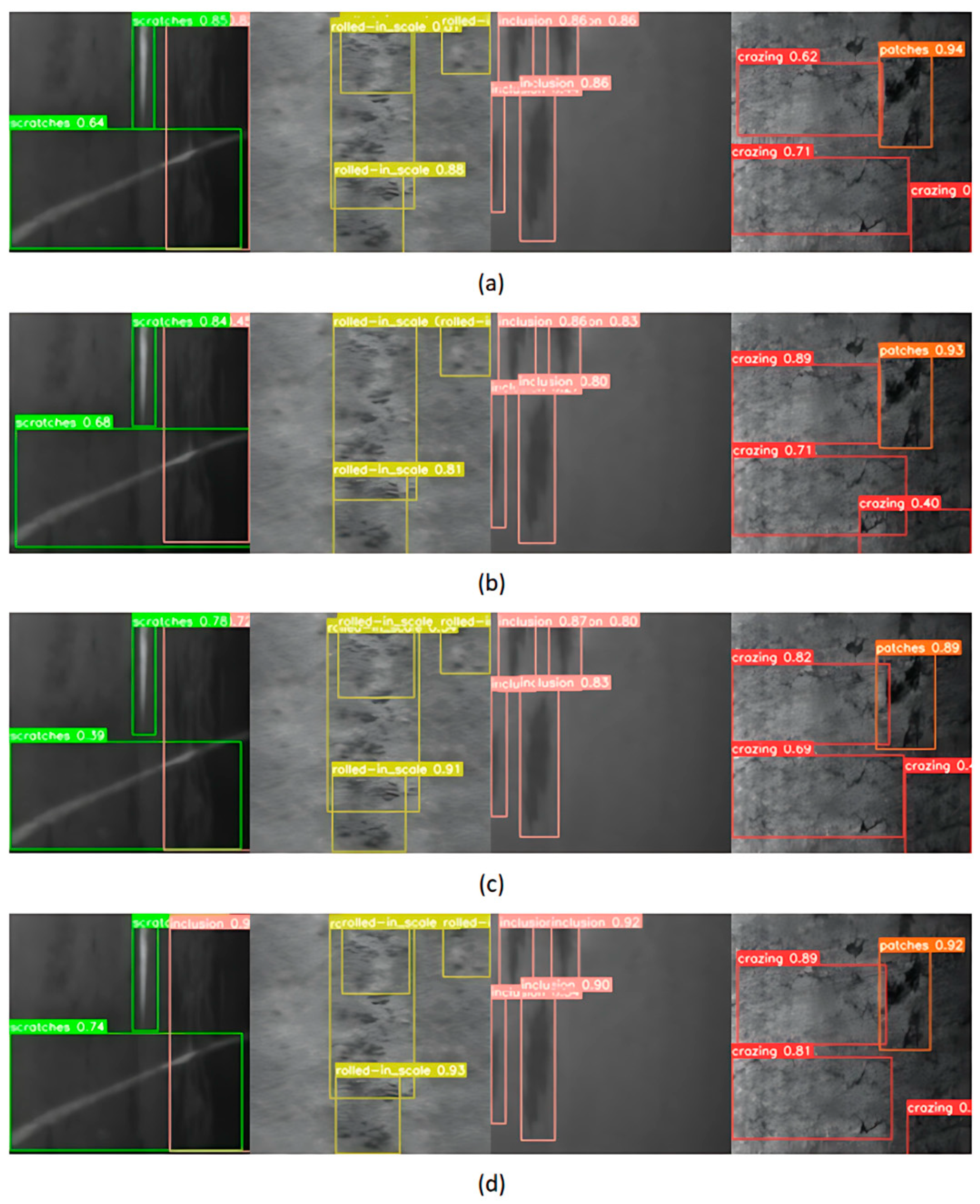
In this section, YOLOv7s, YOLOR, PP-YOLOE, and GCF-Net, which have little difference with the parameters of this model, are selected for visual comparison on the steel dataset. We chose four categories from the steel dataset that exhibit low accuracy in detection for a visual analysis, as illustrated in Figure 10. It can be seen that, compared with other models, this model can accurately identify all kinds of defects, without missing detection, and has the highest confidence. This capability can boost the detection performance for defects that occur across various scales and against intricate backgrounds.
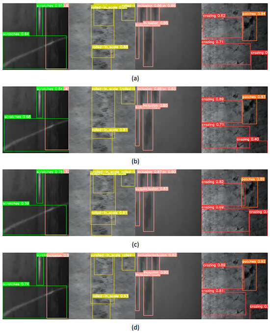
Figure 10.
Visualization effect diagram of images detected by different detectors on the steel dataset: (a) YOLOv7s, (b) YOLOR, (c) PP-YOLOE, and (d) GCF-Net.
4.4. Experiments on PCB Datasets
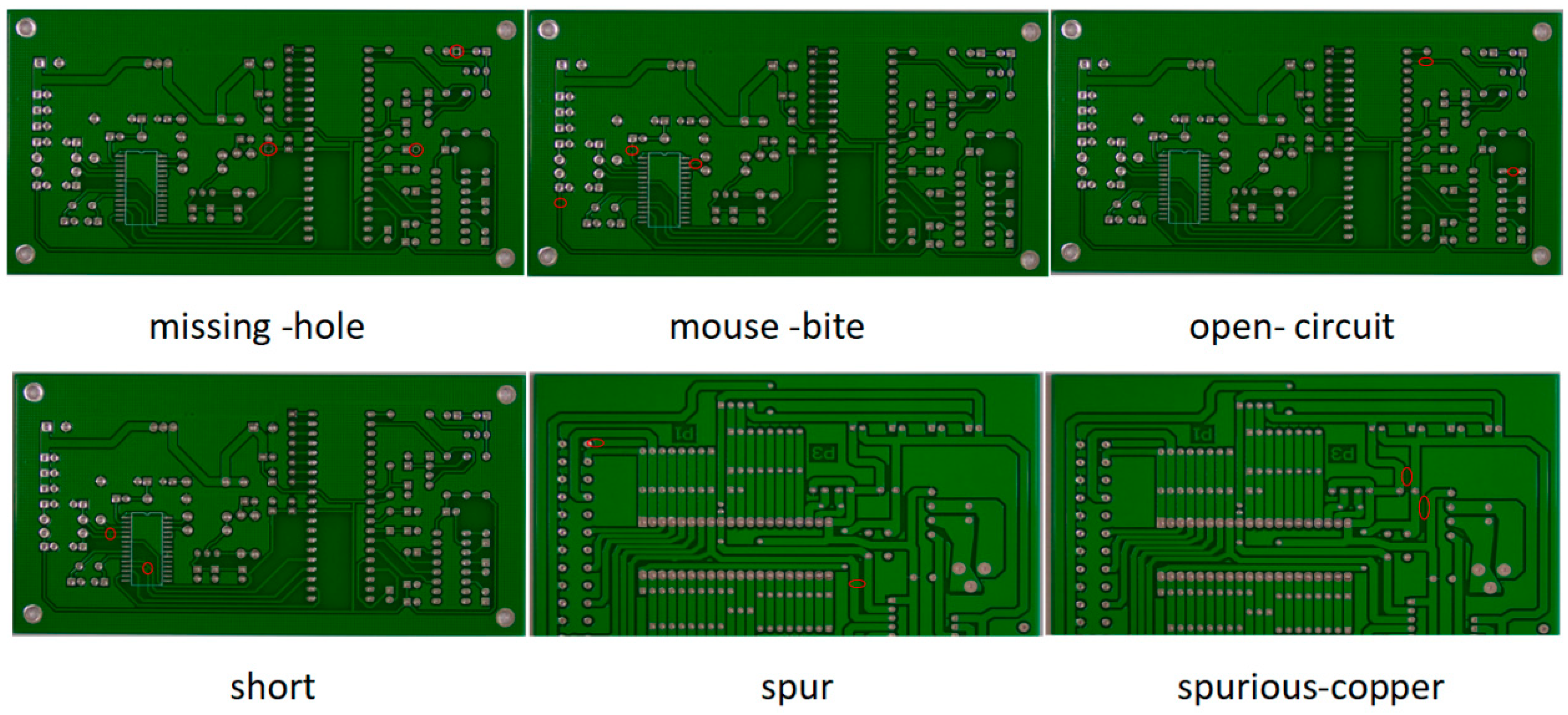
The dataset used in this experiment was the public dataset PCB [46] of the Peking University Intelligent Robot Open Laboratory, which contains six types of defects, namely, missing hole, rat bite, open circuit, short circuit, burr, and residual copper, as shown in Figure 11. Due to the limited number of PCB defect samples in this public dataset, this experiment enhanced the existing samples and expanded the dataset by rotating, flipping, and changing the brightness. The expanded dataset included 345 holes, 345 rat bites, 348 open circuits, 348 short circuits, 345 burrs, and 348 residual copper defects.
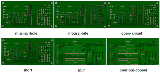
Figure 11.
Visualized images of the PCB dataset, with six defect categories. Defects have been marked with red circles.
4.4.1. Ablation Experiments of Different Modules
In this study, a foundational model was employed to conduct ablation studies on various components within the context of the PCB dataset. As shown in Table 4, using the IFE-Net proposed in this paper to replace the baseline backbone network, R and mAP were increased by 1.9% and 2.2%, respectively. It can be deduced that the IFE-Net, with its interactive feature extraction architecture, is adept at seizing both the nuanced local features and the broader context of images. Consequently, this enhances the model’s ability to detect defects amidst complex backgrounds and noisy environments.
Table 4.
Study on ablation of different components.
CIF-Net, a Cross-Layer Interactive Fusion Network, recovers the detailed information that is typically lost as features are refined over time by integrating nearby layers. At the same time, it uses cross-layer fusion to enhance the interaction between different scales and improve the recognition ability of targets at different scales. R and mAP are improved by 3.4% and 3.9%, respectively. When the IFM is added to the baseline model, R and mAP are increased by 1.3% and 1.3%, respectively. This is because the IFM adjusts the importance of each stitching feature by paying attention to making efficient use of each feature’s information and improving the surface defect detection ability. Incorporating Q_IOU enhances the model’s capacity to discern intricate, small-scale steel defects, thereby boosting the detection accuracy for surface imperfections.
4.4.2. Comparison of Different Neck Networks
Table 5 presents a comparative analysis of the CIF-Net feature fusion network proposed in this paper and the mainstream fusion networks PANet, BiFPN, and RepPAN on the PCB dataset. As can be seen from the table, compared with the other models, the R-value increased by 3.4%, 2.3%, and 1.5%, respectively, and the mAP increased by 3.9%, 2.9%, and 1.4%, respectively. The experimental results can prove the effectiveness of this fusion network in defect detection, because we introduced a Cross-Layer Interactive Fusion Network that compensates for the loss of fine-grained details that occurs during the progressive refinement of features by merging adjacent layers.
Table 5.
Study on ablation of different fusion networks.
4.4.3. Comparative Test in PCB Dataset
For assessing the model’s effectiveness, Table 6 offers a comparative analysis of our approach against prevailing object detection techniques. According to the data in the table, it can be seen that our method surpasses the existing mainstream one-stage and two-stage detection algorithms in terms of mean precision (mAP) and achieves the best results. Compared with YOLOX, YOLOv7s, PP-YOLOE, YOLOR, and other models with little change in parameters, our model achieved the best performance in detection accuracy, and the reasoning speed of the model did not change much, being only slightly lower than that of the YOLOv7s model, but the detection accuracy was much higher than that of the YOLOv7s model. On the whole, GCF-Net achieved the best performance in PCB detection. As shown in Figure 12, compared with the YOLOX, YOLOv7s, PP-YOLOE, and YOLOR models, the R increased by 1.7%, 4.4%, 0.7%, and 3.6%, respectively, and the mAP increased by 1.9%, 4.5%, 0.8%, and 3.9%, respectively, while the reasoning speed was slightly lower than that of YOLOv7.
Table 6.
Comparative experiments of different models in PCB datasets.
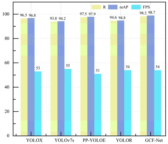
Figure 12.
Comparison of R, mAP, and FPS of different models in PCB datasets.
4.4.4. Visualization Research in PCB Datasets
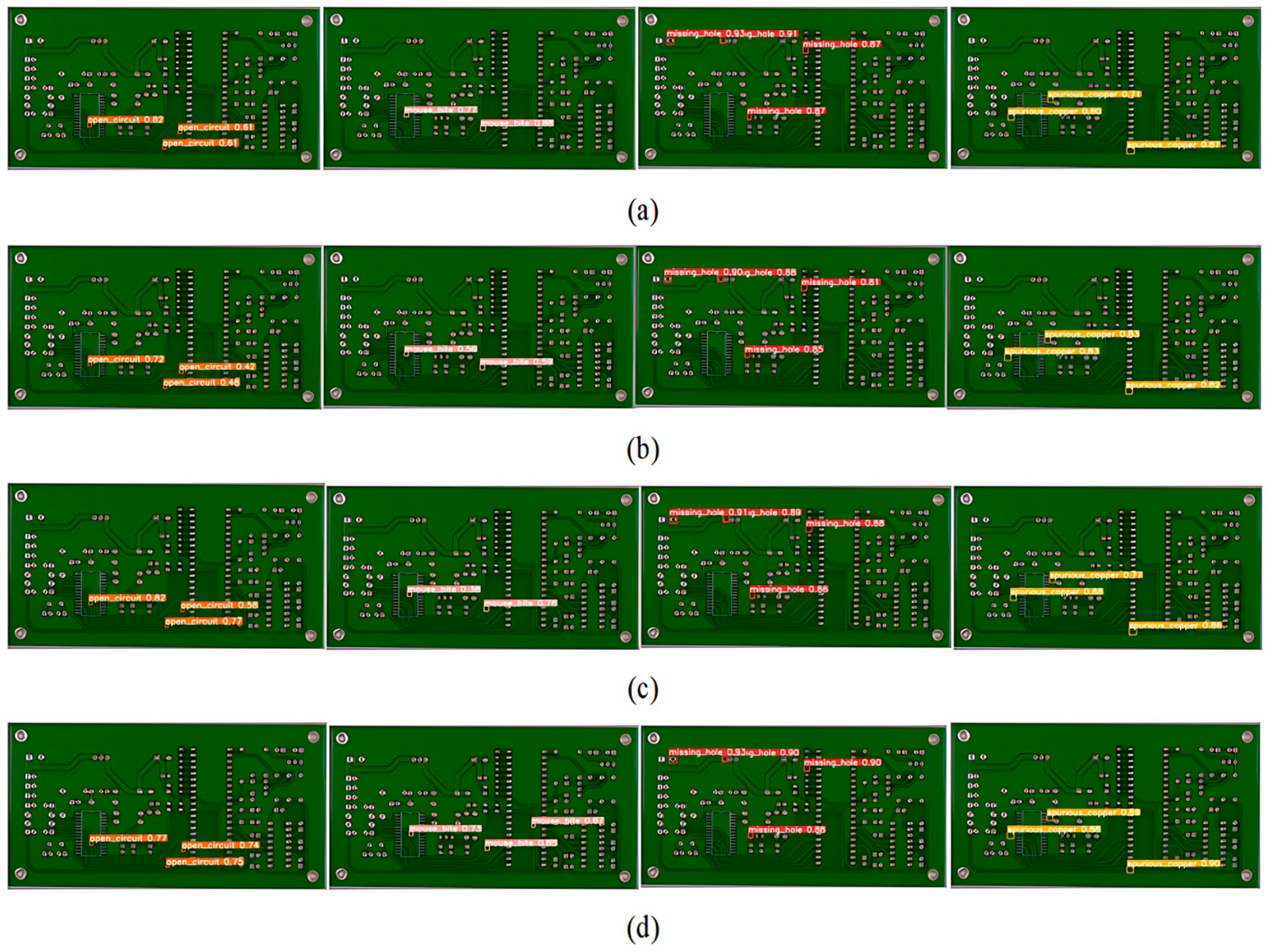
Figure 13 depicts the visual analysis of the PCB dataset. It can be seen that the YOLOv7s, YOLOR, and PP-YOLOE models missed detection in the rat bite defect category. The model proposed in this paper accurately identified all of the defects of complex small targets, and there was no missing detection, which fully shows that GCF-Net can identify and locate small targets in complex backgrounds.
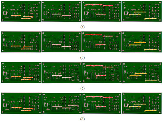
Figure 13.
Visualization effect diagram of images detected by different detectors on the PCB dataset: (a)YOLOv7s, (b) YOLOR, (c) PP-YOLOE, and (d) GCF-Net.
4.5. Steel Dataset Experiment
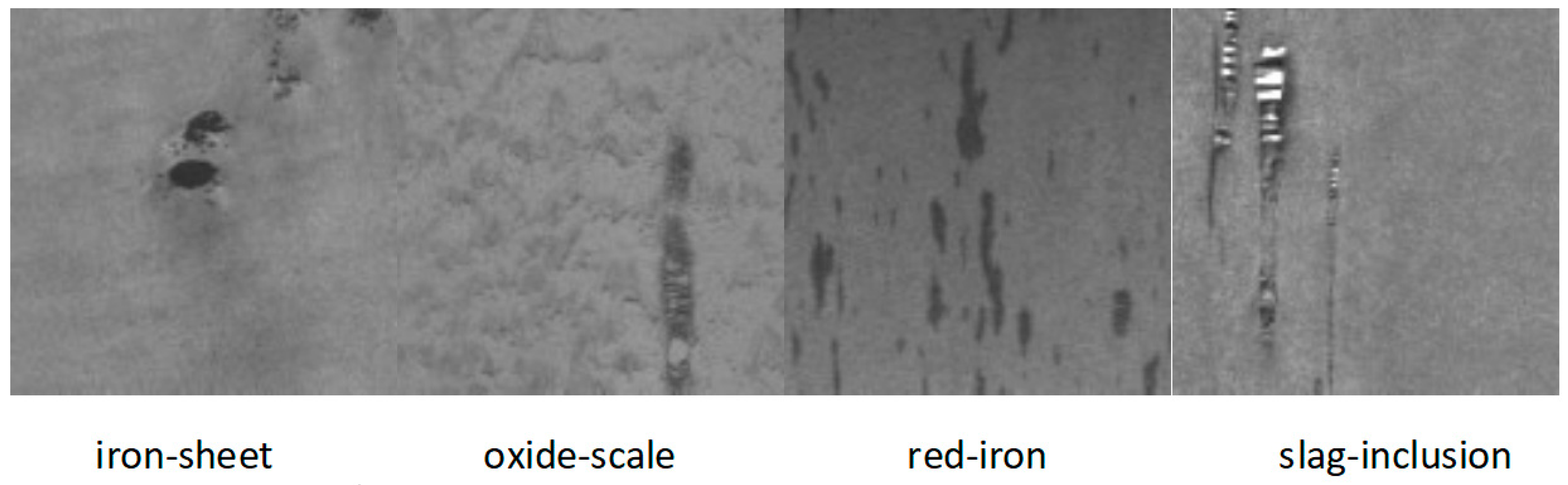
The Steel surface defect dataset [47] has four types of defect, namely, iron-sheet, oxide-scale, red-iron and slag-inclusion, with a total of 1600 pictures. Similarly, the training set and verification set were divided in a 9:1 ratio. Figure 14 shows examples of the surface defects in the Steel dataset.

Figure 14.
Four examples of steel surface defects.
4.5.1. Research on the IFM
In order to verify the effectiveness of the IFM on other datasets, we applied the IFM to the Steel datasets for research. As shown in Table 7. Adding the IFM to the baseline model, R and mAP increased by 0.5% and 1.2%, respectively, proving the effectiveness of the IFM under noise background defects. This is because the IFM adjusts the importance of each mosaic feature by paying attention to make efficient use of all feature information, and then it improves the detection of complex background defects on the Steel dataset.
Table 7.
Influence of IFM module on model checking performance.
4.5.2. Comparative Experimental Analysis
To verify the generalization ability of this model, we compared the GCF-Net model proposed in this paper with commonly used target detection models. As shown in Table 8, GCF-Net achieved the highest mAP value, which was 1.6%, 2.9%, 0.9%, and 2.9% higher than that of the YOLOX, YOLOv7s, PP-YOLOE, and YOLOR models, respectively, with little change in parameter quantities, making it superior to the mainstream one-stage algorithms, as it achieved the highest detection accuracy and was the same as Faster R-CNN in the recall rate R-value. Nevertheless, our model has fewer parameters than Faster R-CNN and achieved a detection speed of 54 FPS, significantly outperforming the two-stage algorithm.
Table 8.
Comparative experiments of different models in Steel dataset.
4.5.3. Ablation Research Between Different Modules
Table 9 shows the ablation experiments of different modules of this model on the Steel dataset, proving the effectiveness of the different modules in this paper. In addition, from the comparison of the sixth, seventh, and eighth lines of the table, it can be concluded that the fusion of different modules improves the detection performance of the model, which proves that different modules are compatible and enhances the detection ability of the model in a complementary way. Adding CIC-Net on the basis of LFN-Net, the mAP value increased by 1.8%. Adding the IFM on the basis of adding LFN-Net and CIC-Net, the mAP value increased by 0.4%. With the addition of Q_IOU loss, the mAP value increased by 0.3%, fully proving the effectiveness of the integration of different modules.
Table 9.
Ablation experiments on the Steel dataset.
4.5.4. Visualization Research in Steel Datasets
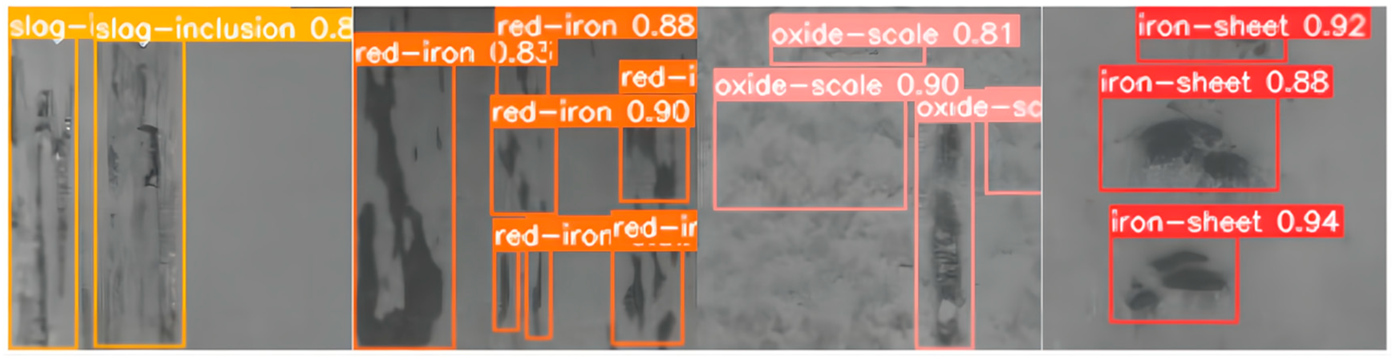
Figure 15 shows the visualization of the GCF-Net model on the Steel dataset. Through image analysis, it can be clearly observed that the model proposed in this study shows high accuracy in identifying defect types in complex backgrounds and correctly detects all defects.
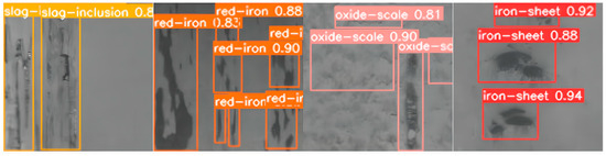
Figure 15.
Detection visualization of the GCF-Net model.
5. Discussion
The purpose of this paper was to design a high-precision defect detection network to improve the problems faced in steel detection, such as complex backgrounds and noise interference, difficulty in accurately detecting complex small targets, and large changes in defects of different scales.
To solve the above problems, we designed an Interactive Feature Extraction network (IFE-Net), a Cross-Layer Interactive Fusion Network (CIF-Net), and an Interactive Fusion Module (IFM) and strengthened the sensitive loss Q_IOU of small targets to improve the detection of different types of defects in steel. A large number of ablation experiments (see Table 1 and Table 2) and contrast experiments (see Table 3) were carried out on the NEU-DET dataset to verify the effectiveness of this model. Compared with the current mainstream one-stage, two-stage, and hybrid detectors, this model was superior to all of the contrast models. By comparing the experiments on the PCB and Steel datasets (see Table 6 and Table 7), the generalization of this model was verified. In addition, the ablation experiments (see Table 4 and Table 5) proved the effectiveness of the different modules proposed in this paper, as well as the robustness of the model. The model proposed in this paper shows a significant competitive advantage in the comprehensive consideration of detection accuracy and speed, which is very important for the defect detection of industrial products.
6. Conclusions
In this paper, a steel surface defect detection network based on global attention perception and cross-layer interactive fusion was proposed to improve the accuracy of defect detection. First of all, we designed the IFE-Net. By introducing the global attention perception module to capture the global contextual information in the image, the detection ability of the model for defects under various background noises and interferences was improved. Then, we introduced a CIF-Net, which supplements the fine-grained information lost in the process of feature refinement through layer fusion, enhancing the recognition ability of multi-scale defect targets. In addition, we also developed an IFM, which adjusts the importance of different mosaic features through the attention mechanism, realizes the efficient fusion of features of different scales, and further improves the detection performance of defects in complex backgrounds. Ultimately, we introduced Q_IOU to boost the sensitivity of the loss functions for small objects, leading to a substantial enhancement in detecting intricate, minor targets on steel surfaces.
Experiments on the NEU-DET dataset proved the effectiveness of different modules, and experiments on the PCB and Steel datasets verified the generalization of this model. In addition, the PCB dataset contains a large number of complex, small target defects, which were used to verify the positioning performance of the Q_IOU proposed in this paper. The Steel dataset is disturbed by complex background noise. Experiments on this dataset verified the effectiveness of the IFM in detecting defects in complex backgrounds. Therefore, the steel surface defect detection network proposed in this paper achieved remarkable results in improving the detection accuracy and reducing the false detection rate, and it proved its universality, providing strong technical support for the quality control of the steel industry.
Although the method proposed in this paper improved the steel defect detection, as a technology relying on supervised learning, it faces the challenge of dataset size and pretreatment requirements, which usually require manual intervention, and the potential of this method cannot be fully tapped when the dataset is insufficient. Therefore, our future research direction will focus on exploring semi-supervised or unsupervised learning strategies to reduce the dependence on a large number of labeled data, which will provide new technical support for industrial product defect detection.
Author Contributions
Conceptualization, W.S. and C.L.; methodology, W.S.; software, C.L.; validation, W.S.; formal analysis, J.D.; data curation, J.D.; writing—original draft preparation, W.S.; writing—review and editing, W.S.; visualization, C.L.; supervision, C.L.; project administration, N.N.; funding acquisition, N.N. All authors have read and agreed to the published version of the manuscript.
Funding
This research was conducted without external funding, utilizing institutional computational resources and open-source tools to ensure cost-effective implementation.
Data Availability Statement
The data used to support the findings of this study are available from the corresponding author upon request.
Conflicts of Interest
The authors declare no conflict of interest.
References
- Bhatt, P.M.; Malhan, R.K.; Rajendran, P.; Shah, B.C.; Thakar, S.; Yoon, Y.J.; Gupta, S.K. Image-based surface defect detection using deep learning: A review. J. Comput. Inf. Sci. Eng. 2021, 21, 040801. [Google Scholar] [CrossRef]
- Tsai, D.M.; Fan, S.K.S.; Chou, Y.H. Auto-annotated deep segmentation for surface defect detection. IEEE Trans. Instrum. Meas. 2021, 70, 1–10. [Google Scholar] [CrossRef]
- Wang, L.; Zhang, Z.; Yin, W.; Chen, H.; Zhou, G.; Ma, H.; Tan, D. Parameters impact analysis of CFRP defect detection system based on line laser scanning thermography. Nondestruct. Test. Eval. 2024, 39, 1169–1194. [Google Scholar] [CrossRef]
- Demir, K.; Ay, M.; Cavas, M.; Demir, F. Automated steel surface defect detection and classification using a new deep learning-based approach. Neural Comput. Appl. 2023, 35, 8389–8406. [Google Scholar] [CrossRef]
- Zhao, C.; Shu, X.; Yan, X.; Zuo, X.; Zhu, F. RDD-YOLO: A modified YOLO for detection of steel surface defects. Measurement 2023, 214, 112776. [Google Scholar] [CrossRef]
- Ling, Q.; Isa, N.A.M.; Asaari, M.S.M. SDD-Net: Soldering defect detection network for printed circuit boards. Neurocomputing 2024, 610, 128575. [Google Scholar] [CrossRef]
- Li, W. Analysis of object detection performance based on Faster R-CNN. J. Phys. Conf. Ser. 2021, 1827, 012085. [Google Scholar] [CrossRef]
- Xu, C.; Shi, C.; Bi, H.; Liu, C.; Yuan, Y.; Guo, H.; Chen, Y. A page object detection method based on mask R-CNN. IEEE Access 2021, 9, 143448–143457. [Google Scholar] [CrossRef]
- Tang, B.; Chen, L.; Sun, W.; Lin, Z. Review of surface defect detection of steel products based on machine vision. IET Image Process. 2023, 17, 303–322. [Google Scholar] [CrossRef]
- Cui, L.; Jiang, X.; Xu, M.; Li, W.; Ly, P.; Zhou, B. SDDNet: A fast and accurate network for surface defect detection. IEEE Trans. Instrum. Meas. 2021, 70, 2505713. [Google Scholar] [CrossRef]
- Li, M.; Wang, H.; Wan, Z. Surface defect detection of steel strips based on improved YOLOv4. Comput. Electr. Eng. 2022, 102, 108208. [Google Scholar] [CrossRef]
- Gao, L.; Zhang, J.; Yang, C.; Zhou, Y. Cas-VSwin transformer: A variant swin transformer for surface-defect detection. Comput. Ind. 2022, 140, 103689. [Google Scholar] [CrossRef]
- Kong, H.; You, C. Improved steel surface defect detection algorithm based on YOLOv8. IEEE Access 2024, 12, 99570–99577. [Google Scholar]
- Du, B.; Wan, F.; Lei, G.; Xu, L.; Xu, C.; Xiong, Y. YOLO-MBBi: PCB surface defect detection method based on enhanced YOLOv5. Electronics 2023, 12, 2821. [Google Scholar] [CrossRef]
- Chen, Y.; Ding, Y.; Zhao, F.; Zhang, E.; Wu, Z.; Shao, L. Surface defect detection methods for industrial products: A review. Appl. Sci. 2021, 11, 7657. [Google Scholar] [CrossRef]
- Gao, Y.; Li, X.; Wang, X.V.; Wang, L.; Gao, L. A review on recent advances in vision-based defect recognition towards industrial intelligence. J. Manuf. Syst. 2022, 62, 753–766. [Google Scholar] [CrossRef]
- Jing, J.; Liu, S.; Wang, G.; Zhang, W.; Sun, C. Recent advances on image edge detection: A comprehensive review. Neurocomputing 2022, 503, 259–271. [Google Scholar] [CrossRef]
- Alzubaidi, L.; Zhang, J.; Humaidi, A.J.; Al-Dujaili, A.; Duan, Y.; Al-Shamma, O.; Santamaría, J.; Fadhel, M.A.; Al-Amidie, M.; Farhan, L. Review of deep learning: Concepts, CNN architectures, challenges, applications, future directions. J. Big Data 2021, 8, 53. [Google Scholar] [CrossRef]
- Miao, T.; Zeng, H.C.; Yang, W.; Chu, B.; Zou, F.; Ren, W.; Chen, J. An improved lightweight RetinaNet for ship detection in SAR images. IEEE J. Sel. Top. Appl. Earth Obs. Remote Sens. 2022, 15, 4667–4679. [Google Scholar] [CrossRef]
- Hou, L.; Lu, K.; Xue, J. Refined one-stage oriented object detection method for remote sensing images. IEEE Trans. Image Process. 2022, 31, 1545–1558. [Google Scholar] [CrossRef]
- Xie, X.; Cheng, G.; Wang, J.; Yao, X.; Han, J. Oriented R-CNN for object detection. In Proceedings of the IEEE/CVF International Conference on Computer Vision, Montreal, QC, Canada, 11–17 October 2021; pp. 3520–3529. [Google Scholar]
- Zhang, T.; Quan, S.; Yang, Z.; Guo, W.; Zhang, Z.; Gan, H. A two-stage method for ship detection using PolSAR image. IEEE Trans. Geosci. Remote Sens. 2022, 60, 1–18. [Google Scholar] [CrossRef]
- Xiao, M.; Yang, B.; Wang, S.; Zhang, Z.; He, Y. Fine coordinate attention for surface defect detection. Eng. Appl. Artif. Intell. 2023, 123, 106368. [Google Scholar] [CrossRef]
- Yang, K.; Chen, T. Lightweight Surface Defect Detection Algorithm Based on Improved YOLOv5. In Proceedings of the 2024 5th International Conference on Mechatronics Technology and Intelligent Manufacturing (ICMTIM), Nanjing, China, 26–28 April 2024; pp. 798–802. [Google Scholar]
- Li, X.; Zheng, Y.; Chen, B.; Zheng, E. Dual attention-based industrial surface defect detection with consistency loss. Sensors 2022, 22, 5141. [Google Scholar] [CrossRef]
- Song, K.; Sun, X.; Ma, S.; Yan, Y. Surface defect detection of aeroengine blades based on cross-layer semantic guidance. IEEE Trans. Instrum. Meas. 2023, 72, 1–11. [Google Scholar] [CrossRef]
- Wang, G.; Gan, X.; Cao, Q.; Zhai, Q. MFANet: Multi-scale feature fusion network with attention mechanism. Vis. Comput. 2023, 39, 2969–2980. [Google Scholar] [CrossRef]
- Zhong, J.; Zhu, J.; Huyan, J.; Ma, T.; Zhang, W. Multi-scale feature fusion network for pixel-level pavement distress detection. Autom. Constr. 2022, 141, 104436. [Google Scholar] [CrossRef]
- Si, C.; Yu, W.; Zhou, P.; Zhou, Y.; Wang, X.; Yan, S. Inception transformer. Adv. Neural Inf. Process. Syst. 2022, 35, 23495–23509. [Google Scholar]
- Wu, X.; Hong, D.; Chanussot, J. UIU-Net: U-Net in U-Net for infrared small object detection. IEEE Trans. Image Process. 2022, 32, 364–376. [Google Scholar] [CrossRef]
- Beeche, C.; Singh, J.P.; Leader, J.K.; Gezer, N.S.; Oruwari, A.P.; Dansingani, K.K.; Chhablani, J.; Pu, J. Super U-Net: A modularized generalizable architecture. Pattern Recognit. 2022, 128, 108669. [Google Scholar] [CrossRef]
- Gong, Y.; Yu, X.; Ding, Y.; Peng, X.; Zhao, J.; Han, Z. Effective fusion factor in FPN for tiny object detection. In Proceedings of the IEEE/CVF Winter Conference on Applications of Computer Vision, Virtual, 5–9 January 2021; pp. 1160–1168. [Google Scholar]
- Liu, S.; Qi, L.; Qin, H.; Shi, J.; Jia, J. Path aggregation network for instance segmentation. In Proceedings of the IEEE Conference on Computer Vision and Pattern Recognition, Salt Lake City, UT, USA, 18–22 June 2018; pp. 8759–8768. [Google Scholar]
- Tan, M.; Pang, R.; Le, Q.V. Efficientdet: Scalable and efficient object detection. In Proceedings of the IEEE/CVF Conference on Computer Vision and Pattern Recognition, Seattle, WA, USA, 14–19 June 2020; pp. 10781–10790. [Google Scholar]
- Wang, Q.; Ma, Y.; Zhao, K.; Tian, Y. A comprehensive survey of loss functions in machine learning. Ann. Data Sci. 2020, 9, 187–212. [Google Scholar] [CrossRef]
- Li, Q.; Jia, X.; Zhou, J.; Shen, L.; Duan, J. Rediscovering BCE Loss for Uniform Classification. arXiv 2024, arXiv:2403.07289. [Google Scholar]
- Zheng, Z.; Wang, P.; Ren, D.; Liu, W.; Ye, R.; Hu, Q. Enhancing geometric factors in model learning and inference for object detection and instance segmentation. IEEE Trans. Cybern. 2021, 52, 8574–8586. [Google Scholar] [CrossRef]
- Northeast. University. Available online: http://faculty.neu.edu.cn/songkechen/zh_CN/zdylm/263270/list/index.htm (accessed on 15 October 2022).
- Ultralytics, 2020. YOLOv5. Available online: https://github.com/ultralytics/yolov5 (accessed on 12 May 2020).
- Zheng, G.; Songtao, L.; Feng, W.; Li, Z.; Sun, J. YOLOX: Exceeding YOLO series in 2021. arXiv 2021, arXiv:2107.08430. [Google Scholar]
- Wang, C.Y.; Bochkovskiy, A.; Liao, H.Y.M. YOLOv7: Trainable bag-of-freebies sets new state-of-the-art for real-time object detectors. In Proceedings of the IEEE/CVF Conference on Computer Vision and Pattern Recognition, Vancouver, BC, Canada, 17–24 June 2023; pp. 7464–7475. [Google Scholar]
- Varghese, R.; Sambath, M. YOLOv8: A Novel Object Detection Algorithm with Enhanced Performance and Robustness. In Proceedings of the 2024 International Conference on Advances in Data Engineering and Intelligent Computing Systems (ADICS), Chennai, India, 18–19 April 2024; pp. 1–6. [Google Scholar]
- Xu, S.; Wang, X.; Lv, W.; Chang, Q.; Cui, C.; Deng, K.; Wang, G.; Dang, Q.; Wei, S.; Du, Y.; et al. PP-YOLOE: An evolved version of YOLO. arXiv preprint 2022, arXiv:2203.16250. [Google Scholar]
- Wang, C.Y.; Yeh, I.H.; Liao, H.Y.M. You only learn one representation: Unified network for multiple tasks. arXiv 2021, arXiv:2105.04206. [Google Scholar]
- Wang, A.; Chen, H.; Liu, L.; Chen, K.; Lin, Z.; Han, J.; Ding, G. Yolov10: Real-time end-to-end object detection. arXiv 2024, arXiv:2405.14458. [Google Scholar]
- Beijing University, P.; PKU-Market-PCB. Available online: https://robotics.pkusz.edu.cn/resources/dataset (accessed on 24 January 2019).
- Zhao, S.L.; Li, G.; Zhou, M.L.; Li, M. ICA-Net: Industrial defect detection network based on convolutional attention guidance and aggregation of multiscale features. Eng. Appl. Artif. Intell. 2023, 126, 107134. [Google Scholar] [CrossRef]
- Liu, X.; Peng, H.; Zheng, N.; Yang, Y.; Hu, H.; Yuan, Y. Efficientvit: Memory efficient vision transformer with cascaded group attention. In Proceedings of the IEEE/CVF Conference on Computer Vision and Pattern Recognition, Vancouver, BC, Canada, 17–24 June 2023; pp. 14420–14430. [Google Scholar]
- Zhao, Y.; Lv, W.; Xu, S.; Wei, J.; Wang, G.; Dang, Q.; Liu, Y.; Chen, J. Detrs beat yolos on real-time object detection. In Proceedings of the IEEE/CVF Conference on Computer Vision and Pattern Recognition, Seattle, WA, USA, 16–22 June 2024; pp. 16965–16974. [Google Scholar]


Disclaimer/Publisher’s Note: The statements, opinions and data contained in all publications are solely those of the individual author(s) and contributor(s) and not of MDPI and/or the editor(s). MDPI and/or the editor(s) disclaim responsibility for any injury to people or property resulting from any ideas, methods, instructions or products referred to in the content. |
© 2025 by the authors. Licensee MDPI, Basel, Switzerland. This article is an open access article distributed under the terms and conditions of the Creative Commons Attribution (CC BY) license (https://creativecommons.org/licenses/by/4.0/).