Concept Paper

Redundancy Determination of HVDC MMC Modules

KEPCO Research Institute, 105 Munjiro Yuseong, Daejeon 305-760, Korea
*
Author to whom correspondence should be addressed.
Electronics 2015, 4(3), 526-537; https://doi.org/10.3390/electronics4030526
Submission received: 30 April 2015 / Revised: 16 July 2015 / Accepted: 29 July 2015 / Published: 4 August 2015
(This article belongs to the Special Issue Multi-Level Converters)

Abstract

:
An availability and a reliability prediction has been made for a high-voltage direct-current (HVDC) module of VSC (Voltage Source Converter) containing DC/DC converter, gate driver, capacitor and insulated gate bipolar transistors (IGBT). This prediction was made using published failure rates for the electronic equipment. The purpose of this prediction is to determinate the additional module redundancy of VSC and the used method is “binomial failure method”.

1. Introduction

An high-voltage direct-current (HVDC) valve module using insulated gate bipolar transistors (IGBTs) contains several thousand electronic components. A quantitative availability analysis and a quantitative reliability analysis have been performed for use in cost-reliability tradeoff decisions in the design of the HVDC valve module.
Reliability is defined as the ability of an item to perform the required function under stated conditions for a certain period of time, which is often measured by probability of survival and failure rate. It is relevant to the durability (i.e., lifetime) and availability of the item. The essence of reliability engineering is to prevent the creation of failures. The deficiencies in the design phase have effect on all produced items and the cost to correct them is progressively increased as the development proceeds. The reliability engineering has emerged as an identified discipline since the 1950s with the demands to address the reliability issues in electronic products for military applications. Since then, much pioneer work has been devoted to various reliability topics. One of the main streams is the quantitative reliability prediction based on empirical data and various handbooks released by military and industry [1,2]. Another stream of the discipline focuses on identifying and modeling of the physical causes of component failures. This paper presents a comprehensive overview of the reliability of power electronic systems. The final purpose of this paper is to decide the redundancy number of VSC module.

2. Reliability Prediction Metrics

The first step in evaluating and improving system reliability is to determine what metrics to analyze. Because metrics always reflect the design goals, any information that is utilized to determine the metrics shall be based on requirements from customers and careful consideration of intended applications. The commonly adopted metrics for the evaluation of power electronic systems encompass reliability, failure rate, mean time to failure (MTTF), mean time to repair (MTTR) and availability [3].

2.1. Reliability

Reliability is defined as the probability that an item (component, subsystem, or system) performs required functions for an intended period of time under given environmental and operational conditions [3]. The reliability function R(t) represents the probability that the system will operate without failures over a time interval [0, t]. The reliability of a system is dependent on the time in consideration. The reliability typically decreases as the time in consideration progresses. For commercial products, the time should cover the warranty time.

2.2. Failure Rate

The failure rate of an item is an indication of the “proneness to failure” of the item after time t has elapsed. Figure 1 shows a typical failure rate curve as a function of time, which is commonly known as the bathtub curve [1,3]. The shape of the bathtub curve in Figure 1 suggests that the life cycle of an item can be divided into three different periods: the development period, the useful life period, and the wear-out period.
Figure 1. Typical failure rate curve (Bathtub curve).
Electronics 04 00526 g001
Although an item is subjected to quite extensive test procedure and much of the infant mortality is removed before they are put into use, undiscovered defects in an item during the process of design or production lead to the high failure rate in the burn-in period. When the item survives in the initial burn-in period, the failure rate tends to stabilize at a level where it remains relatively constant for a certain period of time before the item begins to wear out. While in the wear-out period, systems have finished their required missions. Therefore, the failure rate in useful life time is important to carry out reliability analysis. The failure rate λ(t) is related to the reliability function R(t) by
λ ( t ) = lim t t R ( t ) R ( t + t ) R ( t ) t = 1 R ( t ) d R ( t ) d t
where Δt is a time interval with Δt > 0. The reliability R(t) is determined from the failure rate λ(t) with the consideration of R(0) = 1, i.e., the item is fully functional at the initial state R(t).
R ( t ) =  e 0 t λ ( τ ) dτ 
In many reliability models, the failure rates of components and subsystems are assumed to be independent of time, although this assumption has limitations [4]. With the assumption of λ(t) = λ, (2) is simplified to
R ( t ) =  e λ ( t )
The failure rate is then estimated from the mean number of failures per unit time, which is expressed in failures in time (FIT)
1  FIT  =   10 9 ( failure / hour )  

2.3. Mean Time to Failure

The MTTF is the expected time before a failure occurs. Unlike reliability, MTTF does not depend on a particular period of time. It gives the average time in which an item operates without failing. MTTF is a widely quoted performance metric for comparison of various system designs. This indicator reflects life distribution of an item. Nonetheless, it does not convey the information that a longer MTTF than the mission time means that the system is highly reliable within mission time. The relationship between MTTF and reliability function is described by [3]
MTTF  = 0 +  R ( t ) d t
where R(t) is the reliability function. When the failure rate λ(t) is constant λ, the expression for MTTF is simplified to
MTTF  = 1 λ

2.4. Mean Time to Repair

The (MTTR) is the mean repair time that it takes to eliminate a failure and to restore the system to a specified state. The repair time depends on maintainability, such as effective diagnosis of faults, replaceable components at hand, and so on.

2.5. Availability and Average Availability

The availability is the probability that a system will be functioning at a given time. The average availability denotes the mean portion of the time the system is operating over a given period of time. For a repairable system, if it is repaired to an “as good as new” condition every time it fails, the average availability is
A avg = MTTF MTTF + MTTR  
Therefore, availability improvement entails increasing MTTF and decreasing MTTR. The main limitation associated with the metric of average availability lies in the fact that it cannot reflect frequency of failures or maintenances required.

3. Reliability Assessment of Power Electronic Systems

Reliability evaluation is important for design and operation management of the systems. Quantitative assessment of reliability for power electronic converters is essential in determining whether a particular design meets certain specifications. It also serves as a criterion to compare different topologies, control strategies, and components. Moreover, the accurate reliability prediction gives a valuable guidance to management of the system operation and maintenance. All reliability analysis involves some forms of models, which are either at the component level or at the system level [3].

3.1. Component-Level Reliability Models

For power electronic systems, reliability research at the component level has been mainly focused on failure rate models for the key components in power circuits, such as power semiconductors, capacitors, and magnetic devices. Field experiences have demonstrated that electrolytic capacitors and power switching devices such as insulated gate bipolar transistors (IGBTs) and metal oxide field effect transistors (MOSFETs) are the most vulnerable components [3]. Empirical-based models, which typically rely on observed failure data to quantify model variables, are most widely employed to analyze the reliability of components. The premise is that the valid failure-rate data are readily available either from field applications or from laboratory tests.

3.2. System or Subsystem-Level Reliability Models

A system-level reliability model presents a clear picture of functional interdependences and provides a framework for developing quantitative reliability estimates of systems to guide the design tradeoff process. Several methodologies to quantify the reliability metrics of power electronic converters have been introduced. They can be categorized into three types of reliability models: part-count methods, combinatorial models, and state-space models.
(1) Part-Count Models: The main advantage of part-count method lies in its simplicity. A part-count model can provide adequate reliability estimation for small systems. It is also an effective approach to reliability comparison among different power electronic system architectures at the beginning of design stage. However, for the systems that can tolerate some failures or that can be repaired, the approach leads to over conservative results [3].
(2) Combinatorial Models: Combinatorial models are extensions to part-count models and include fault trees, success trees, and reliability blocks diagrams. These methods can be used to analyze reliability of simple redundant systems with Journal of Power Electronics perfect coverage. Fault tree has been used to analyze reliability of electric drive systems. Unfortunately, combinatorial models cannot reflect the details of fault-tolerant systems, such as repair process, imperfect coverage, state rates, order of component failures, and reconfiguration [3].
(3) Markov Model: The Markov model is based on graphical representation of system states that correspond to system configurations, which are reached after a unique sequence of component failures and transitions among these states [3]. The system is said in failure-free state when all components are nonfaulted. The system can evolve from the failure other states when faults occur to the components. Markov chain is a very effective approach to quantify the reliability of fault-tolerant systems. This approach can cover many features of fault-tolerant systems, such as sequence of failures, failure coverage, and state-dependent failure rates. There are some limitations associated with Markov model. One important property of Markov process is that the transition probability from one state to another does not depend on the previous states but only on the present state. Hence, the Markov model cannot be used to evaluate the system reliability when components have time-varying failure rates. Another shortcoming is that state space grows exponentially with the number of components. For large system, it is difficult to generate the Markov model from the system functional description and components failure analysis. The challenge of applying Markov models to increasingly complicated systems can be clearly appreciated in a high-power multilevel converter that may have hundreds of components and subsequent failure mode transitions.
(4) Binomial Distribution Model: The binomial failure model is an important probability model that is used when there are two possible outcomes (hence “binomial”). In a binomial experiment there are two mutually exclusive outcomes, often referred to as “success” and “failure”. Probability of success is p, the probability such an experiment whose outcome is random and can be either of two possibilities, “success” or “failure”, is called a Bernoulli trial. Binomial Distribution Model is defined as [1,4,5]:
P ( x   =   success ) = n ! x ! ( n x ) ! p x ( 1 p ) ( n x )
where, n is the number of trials or observations, x is the number of “success” and p is the probability of “success”.

4. Module Reliability of VSC Multilevel Converter

The development of power electronics and controllable device in power system is rapidly expanding the field of applications for voltage source converter (VSC)-based HVDC technologies. VSC HVDC system is based on insulated-gate bipolar transistor (IGBT) and the topology is multilevel topologies. The recent trends on multilevel converters for HVDC systems use modular multilevel converter (MMC) topology which connects two-level converter modules in cascade to achieve the desired AC voltage.
The HVDC model presented in this paper considers 600MW VSC-HVDC link with two MMCs, including about 400 SMs per phase. 
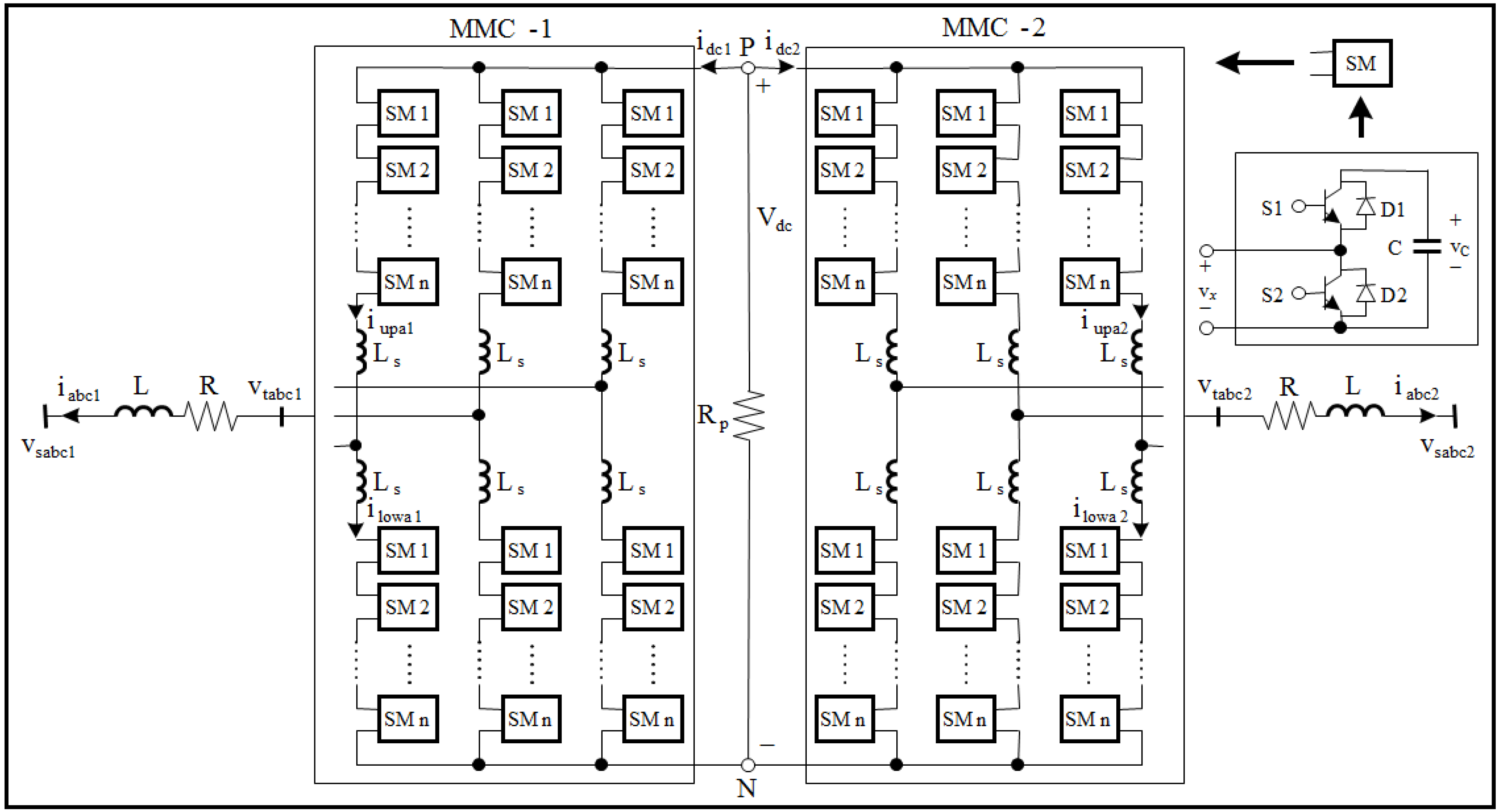
Figure 2 shows the MMC topology where each SM (submodule) contains a capacitor and two insulated-gate bipolar transistor (IGBT) switches (S1 and S2). At any instant during normal operation, only one of the two switches (S1 or S2) is ON. As a result, when the switch S1 is ON (S2 is OFF), the voltage of the SM is and when the switch S2 is ON (S1 is OFF), the SM voltage is zero. The numbers of submodule of MMC depend on the selected IGBT devices, in this paper, 3 kinds of IGBT, as 1.6 kV, 1.8 kV and 2 kV were considered. The numbers of submodules required in the target system are Table 1.
Table 1. Numbers of Submodules.
Module VoltageNumber of Submodule
1.6 kV375
1.8 kV334
2.0 kV300
Figure 2. Modular Multilevel Converter Topology.
Electronics 04 00526 g002
In order to estimate the number of additional modules required in each converter arm an estimate of the system reliability is made. This will then need to be refined by substituting the values with values obtained after more calculation and revising the circuit to reduce areas that are vulnerable.
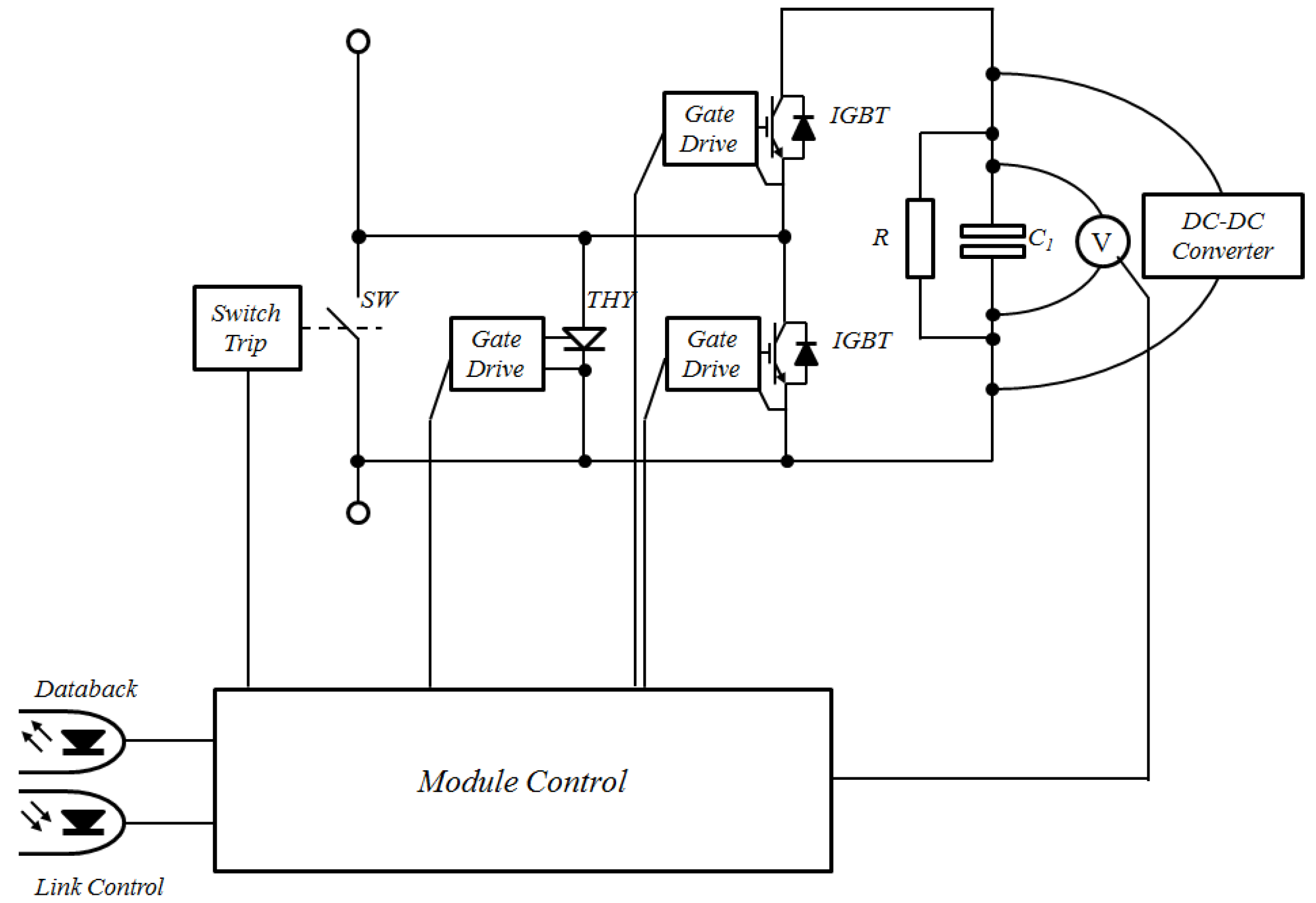
The components such as the thyristor and the shorting switch shown by Figure 3 are only operated under exceptional circumstances and so will not be included in the main calculation at this time. The main source for component reliability is the maker’s catalogues and the failure rate data of SM of the MMC is presented in Table 2 [6]. The values are presented in units of “Failures In Time”, which are defined as failures per billion hours (1e−9 failures/hour).
Figure 3. Submodule of modular multilevel converter (MMC) Voltage Source Converter.
Electronics 04 00526 g003
Table 2. Failure Rate Data.
ComponentNo.Failure Rate (FIT)Total Failure RateComments
- IGBT and gate drive24080Power Circuit
- Thyristor and gate drive14747
- Bypass Switch110001000
- Power Capacitor11010
- Power Resistor1265265
- Custom IC1150150Control
- Optical Rx/Tx2100200
- IC Circuit11313
- Ferrite Core22244Power Supply
- Switching Power Supply110001000
As stated above only the values shown rows 3, 6, 7, 9–11, 13 and 14 in Table 2 are combined to give the failure rate of the module. If 𝛾0 to 𝛾11 represent the values from the “Total Failure Rate” column as elements in a vector the expression becomes:
𝜆M = 𝜆0 + 𝜆3 + 𝜆4 + 𝜆6 + 𝜆7 + 𝜆8 + 𝜆10 + 𝜆11 = 1.762 × 10³ [FIT]
The mean time to failure [MTTF] then becomes:
1 λ M = 64.744   [ y e a r ]
Since this reflects a random event it is more meaningful to convert it to an value representing the availability of the module over a given time span, and by this obtain an estimate of the availability of the complete converter system over its life. This is commonly done by expression values in terms of “Unavailability”, Q:
Q ( t ) = 1 e λ t  
where “t” is the “time at risk”. Thus, assuming full time operation, over the three-year maintenance period the proportion of the all modules in the target MMC HVDC arm to fail will be 4.5%, while over the 30-year life of the equipment, 37 % of the modules will have failed.
This equation can be adapted further to relate a service life and the maintenance period:
Q ( t ) = λ λ + μ ( 1 e ( λ + μ ) t     )
where “t” is the overall time at risk, in this case the equipment life, and “μ” is the maintenance rate, that is, 1/(3years). As would be expected the result is very similar to that above for the 3-year maintenance period, thus, 4.4% of the modules will fail.
To determine the availability of a complete inverter limb of “n” modules in which “m” modules can be allowed to fail before the limb fails the Binomial Failure Model needs to be used:
Q = N ! k ! ( N k ) ! i = k N ( q k ( 1 q N k ) )
When N is large, then the binomial distribution is well approximated by the normal distribution [7].
C k N p k q N k 1 2 π N p q e ( k N p ) 2 2 N p q
where ,   C k N = N ! k ! ( N k ) !
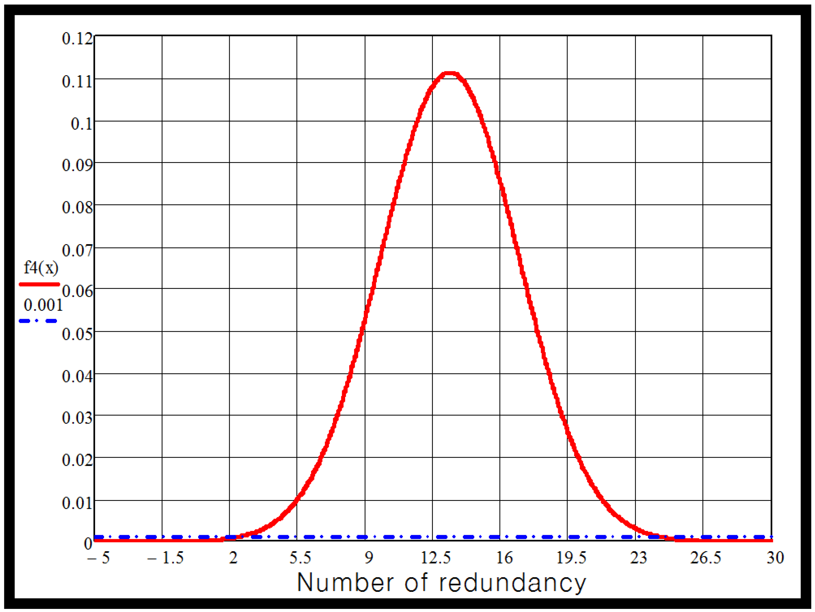
The unavailability for a single inverter arm for the target system has been designed to operate with a minimum of 334 modules, the unavailability of the system according to redundant modules increment is shown in Figure 4.
Figure 4. Unavailability function for the target system with 334 modules according to redundant modules increment.
Electronics 04 00526 g004
In order to determinate the number of the redundant modules for MMC, several scenarios are considered following as:
  • Maintenance periods are 1 year, 2 years and 3 years
  • IGBT devices used are 1.6 kV, 1.8 kV and 2 kV
  • FIT of DC/DC converter changed 1000 to 500
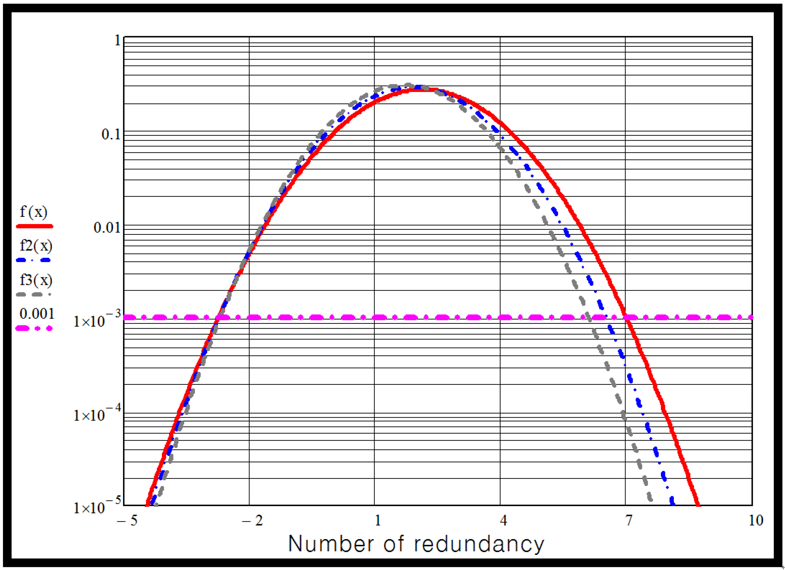
Figure 5 shows the graph of MMC valve unavailability for several IGBT valves against numbers of modules in case of 1-year maintenance. In this case, the unavailability is 0.00568. To achieve better than 99.9% availability requires:
seven modules for a 1.6 kV IGBT device,
six modules for a 1.8 kV IGBT device,
five modules for a 2 kV IGBT device
Figure 5. Unavailability function for MMC valve in case of 1-year maintenance.
Electronics 04 00526 g005
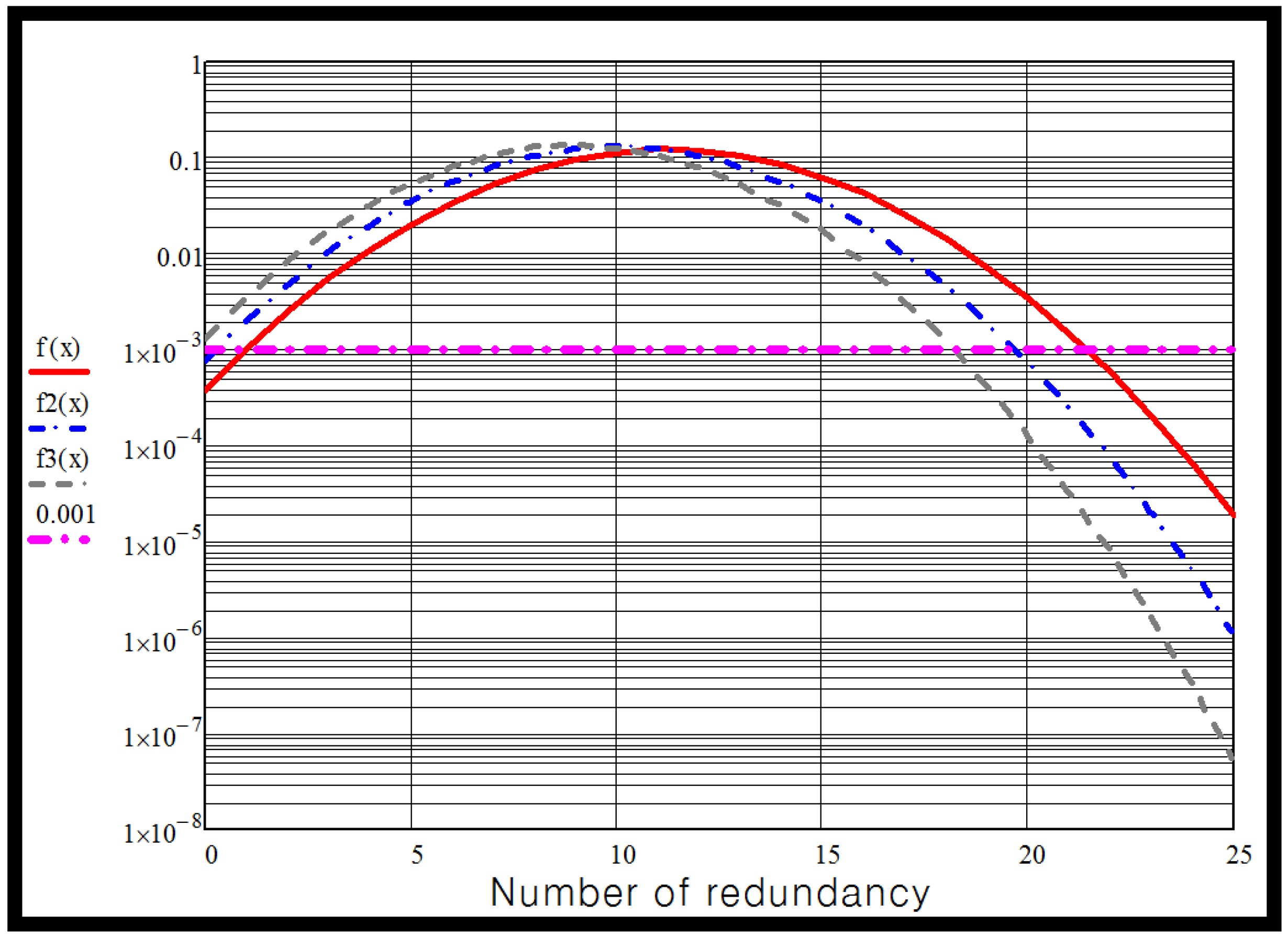
Figure 6 shows the graph of MMC valve unavailability for several IGBT valves against numbers of modules in case of 2-year maintenance. In this case, the unavailability is 0.0299. To achieve better than 99.9% availability requires:
22 modules for a 1.6 kV IGBT device,
20 modules for a 1.8 kV IGBT device5,
17 modules for a 2 kV IGBT device
Figure 6. Unavailability function for MMC valve in case of 2-year maintenance.
Electronics 04 00526 g006
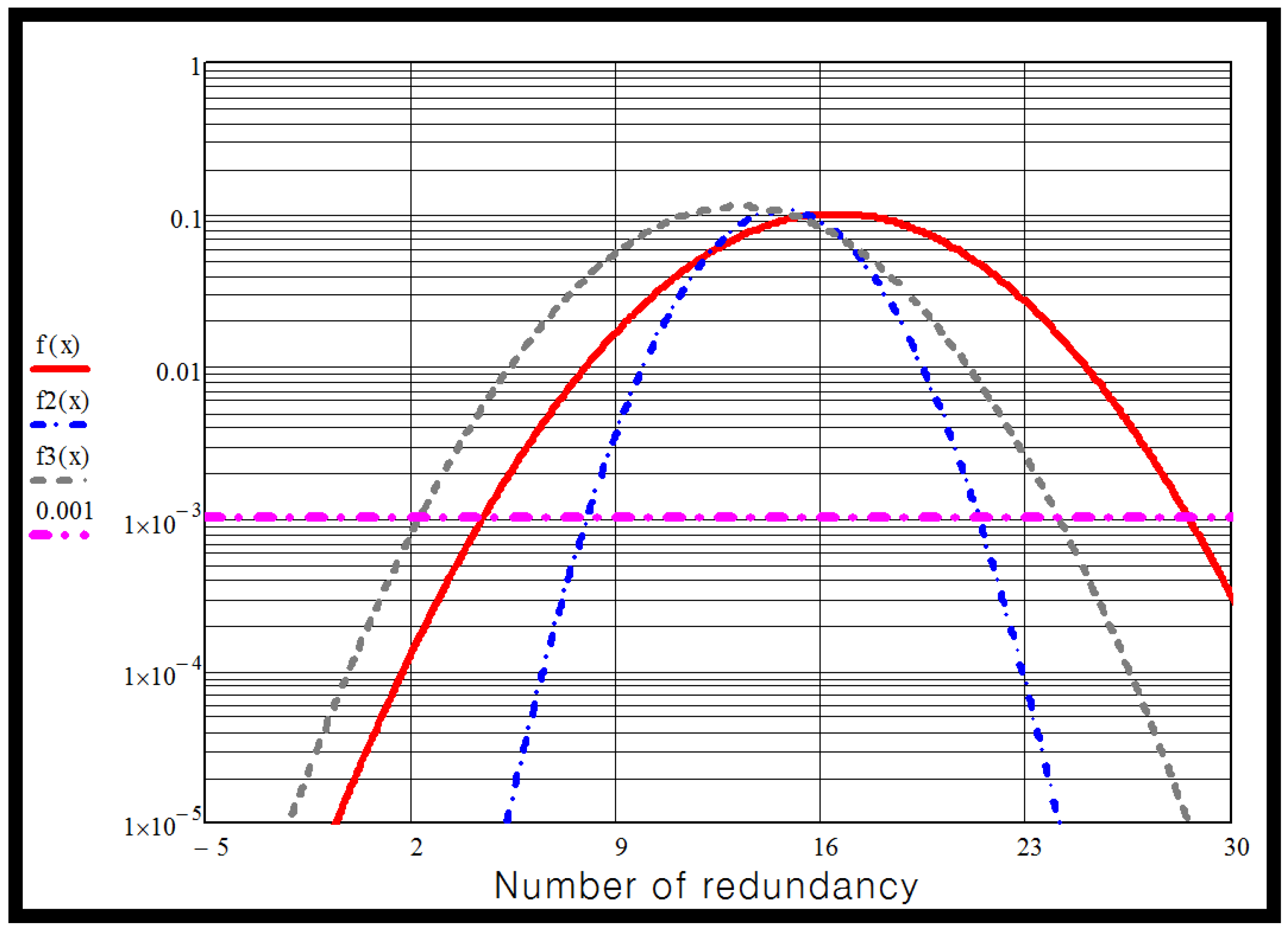
Figure 7 shows the graph of MMC valve unavailability for several IGBT valves against numbers of modules in case of 3-year maintenance. In this case, the unavailability is 0.044. To achieve better than 99.9% availability requires:
28 modules for a 1.6 kV IGBT device,
25 modules for a 1.8 kV IGBT device5,
20 modules for a 2 kV IGBT device
Figure 7. Unavailability function for MMC valve in case of 3-year maintenance.
Electronics 04 00526 g007
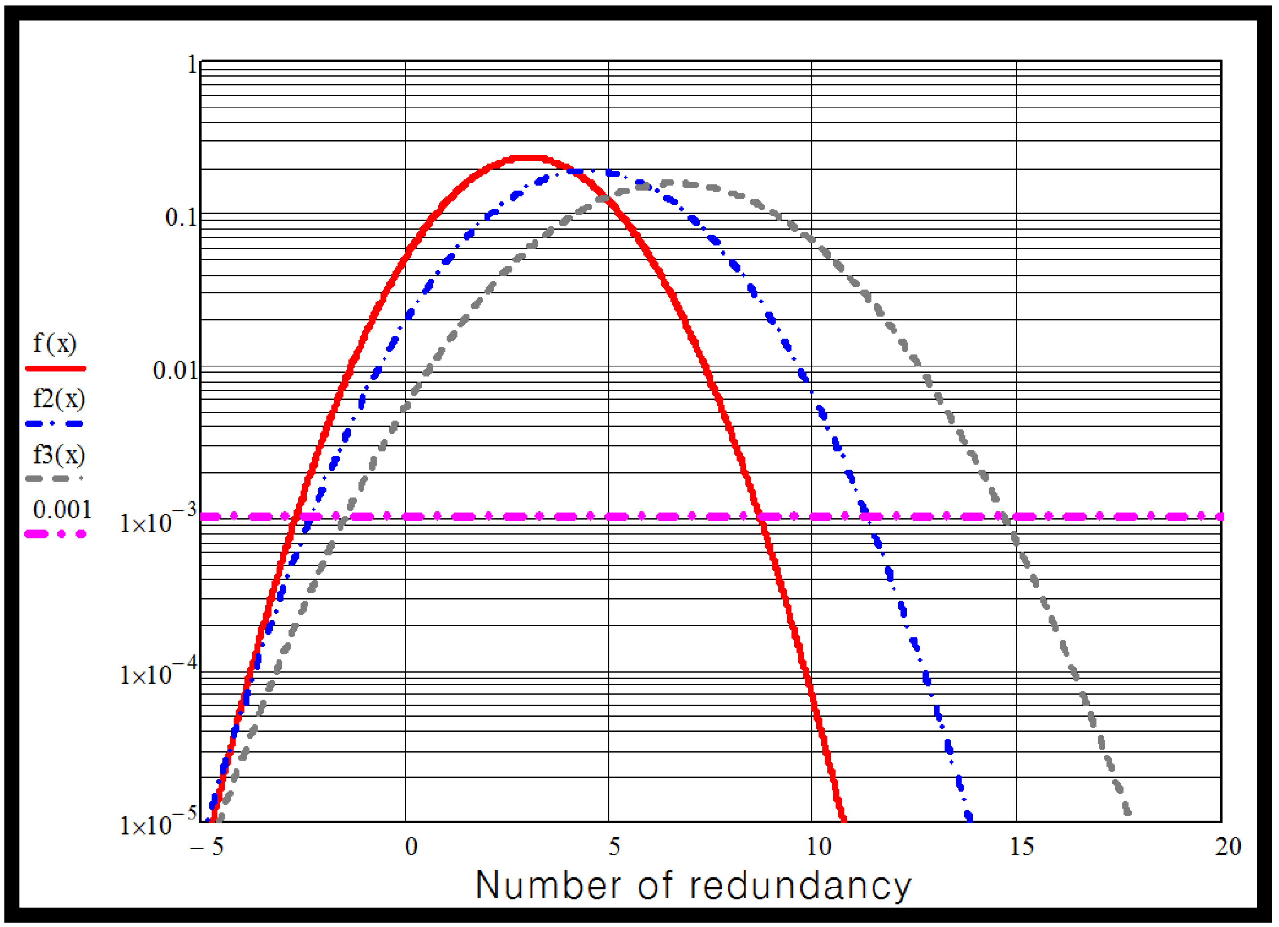
The graph of MMC valve unavailability but with the DC/DC converter failure rate reduced to 500FIT is shown in Figure 8. In this case, the rate of IGBT is 2 [kV] with 300 modules. This shows the equivalent module requirement to be:
7 modules for a 1-year maintenance interval,
12 modules for a 2-year maintenance interval,
15 modules for a 3-year maintenance interval.
Figure 8. Unavailability function for MMC valve with failure rate of DC/DC converter = 500.
Electronics 04 00526 g008
Consequently, the number of MMC module for the maintenance and the range of mean capacitor voltage is given in Table 3.
Table 3. Additional modules against maintenance period and module voltage.
Module VoltageNo. of ModuleAdditional Cells Against Maintenance Period
1 Year2 Years3 Years
1.6 kV37572228
1.8 kV33462025
2.0 kV30051720

5. Conclusions and Discussion

A comprehensive review of the reliability of power electronic converters has been carried out with the intention to provide a clear picture of the current status of this particular research field. The conclusion of this paper is that the additional number of modules depends on the maintenance periods and MMC reliability factor. In MMC valve, if the biggest FIT values of the valve components are reduced, the redundant number of the MMC valve can be also reduced.

Acknowledgments

The authors would like to thank the Alstom engineer, M. Ashraf for supporting in this paper.

Author Contributions

Chanki Kim contributed to the reliability analysis of MMC valve and wrote the first version paper. All authors revised and edited the paper.

Conflicts of Interest

The authors declare no conflict of interest.

References

  1. Department of Defense. Military Handbook: Electronic Reliability Design Handbook; MIL-HDBK-338B1; Department of Defense: Washington, DC, USA, 1998.
  2. Department of Defense. Military Handbook: Reliability Prediction of Electronic Equipment; MIL-HDBK-217F; Department of Defense: Washington, DC, USA, 1991.
  3. Song, Y.; Wang, B. Survey on Reliability of Power Electronic Systems. IEEE Trans. Power Electron. 2013, 28, 591–604. [Google Scholar] [CrossRef]
  4. Høyland, A.; Rausand, M. System Reliability Theory: Models and statistical methods; Wiley: New York, NY, USA, 1994. [Google Scholar]
  5. Dummer, G.W.A. Electronics Reliability—Calculation and Design: Electrical Engineering Division; Pergamon: Oxford, UK, 1966. [Google Scholar]
  6. Voltage Source Converter Development Engineering Report; AREVA: Paris, France, 2008.
  7. Boas, M.L. Mathematical Methods in the Physical Sciences, 3rd ed.; Wiley: New York, NY, USA, 2005. [Google Scholar]

