Spectrum Values in Suburban/Urban Environments above 1.5 GHz

Abstract

Frequency bands higher than 3 GHz will be allocated for 5G telecommunication services. Therefore, investigating the spectrum values at these frequency bands is important for developing an appropriate deployment strategy. In this paper, spectrum values above 1.5 GHz are investigated in suburban and urban environments. In the suburban environment, the relative spectrum values at different positions in a cell are analyzed for frequencies ranging from 500 MHz to 1.5 GHz, 1.5 GHz to 3 GHz, and 3 GHz to 11 GHz. In the urban environment, the maximum achievable capacity of users is calculated for frequencies ranging from 500 MHz to 40 GHz. Numerical results show that spectrum values at lower frequency bands below 5 GHz present higher values at the cell-edge in the suburban environment and in non-line-of-sight (NLoS) situations in the urban environment. However, higher frequency bands have nearly the same impact as low frequency bands at the cell center in suburban environments above 5 GHz but show advantages in outdoor urban environments with line-of-sight (LoS) above 20 GHz. It should be noted that 3.5 GHz shows the highest value in NLoS situations and the indoor domain environment in UMi scenarios, while 28 GHz gives the optimum value at the cell-center and indoor areas with LoS in UMa scenarios. When considering the spectrum value for different frequency bands, the primary consideration should be whether the environment is NLoS or LoS, and the secondary consideration should be whether the environment is indoor or outdoor.

1. Introduction

The electronics and communications industry has had a huge impact on the national economy [1]. Radio frequency (RF) is a frequency or band of frequencies ranging from 10 kHz to 300 GHz used for radio communications. The RF spectrum is the backbone of all telecommunication services and this rare and precious resource has one of the highest economic values in the country [2]. It is critical for the regional regulators or service providers to know the value of different frequency bands so as to make policies, manage cellular market, and deploy cellular networks. Therefore, for both regulators and carriers, the estimation of spectrum value and comparisons of the estimate are very important when additional new bands are allocated for new services such as fifth-generation (5G) telecommunications technology. There was a myth that in policy circles that had many believing spectrum value was not related to the frequency and all spectrums were of equal value [3]. The truth is that the spectrum value is not only selected based on the verities of economic issues in [1] but also technically by the frequency of the spectrum itself. Frequency determines the physical properties of radio waves, which result in how far the radio wave can be reached and how much strong signal can be received. These key parameters greatly affect network coverage and capacity which directly impact on the cost and revenue of service providers.

The estimation of radio spectrum value has been widely studied by economists and financial analysts using the three general techniques Market Comparable, discounted cash flow (DCF), and Econometrics [4]. However, the spectrum value has rarely been investigated from the perspectives of mobile communication engineering. In [3], engineering-economic approaches of quantifying and comparing the spectrum values were proposed, and the frequency spectrum ranging from 500 MHz to 1.5 GHz was investigated in rural, suburban and urban settings. However, the investigation in [3] did not cover frequencies other than 500 MHz to 1.5 GHz. Furthermore, the numerical results did not include the urban scenario, where most of the population is located. Though current cellular systems are mainly operated at frequency bands lower than 3 GHz, the higher frequency spectrum up to millimeter-wave (mmWave) bands is also under consideration for 5G deployment [5].

Radio propagation is the behavior of radio waves travelling from one place to another, which are affected by the phenomena of reflection, refraction, diffraction, absorption, polarization, and scattering. Empirical propagation models based on observations and measurement are broadly used in feasibility studies and initial deployment for cellular network planning, to predict the attenuation of an electromagnetic wave (path loss) [6]. The Hata model was proposed early as an empirical formulation based on data from the Okumura Model [7], which is known to be suitable for frequency bands from 150 MHz to 1.5 GHz. The IEEE working group 802.16 proposed a standard that employed frequency bands up to 11 GHz using the Stanford University Interim (SUI) channel models developed by Stanford University [6]. As even higher frequency bands are required for the 5G system, it is necessary to evaluate new propagation models to determine their feasibility. A 3D path loss model was proposed by 3GPP extending from previous channel models such as the 3D SCM model (3GPP TR 36.873) and the IMT-Advanced model (ITU-R M.2135) [8]. The 3D model supports frequency bands from 500 MHz to 100 GHz in the urban environment and includes various parameters such as penetration loss, shadow fading, and environment heights. In another of our research work [9], the spectrum value of frequency bands ranging from 1.5 GHz to 11 GHz in rural environment is analyzed by using SUI model and 3GPP 3D model [8].

In this paper, the basic approach in [3] is referenced to provide the suburban scenario numerical results but with several expansions and a novel user classification method designed for urban scenario, as described below:

• Much wider frequency bands ranging from 500 MHz to 40 GHz are investigated. In suburban environments, 500 MHz to 1.5 GHz, 1.5 GHz to 3 GHz, and 3 GHz to 11 GHz using Hata and SUI models are investigated. For urban environments, 500 MHz to 40 GHz using the 3D propagation model by 3GPP is evaluated.
• For urban environments, eight types of users are considered under conditions of non-line-of-sight (NLoS) or line-of-sight (LoS), indoor or outdoor, and user location in the cell. The variation of signal propagation due to various factors is one of the main technological challenges in the spectrum management field [10]. It is also important to consider diverse user conditions, especially for indoor environments, where most data traffic is generated but users experience poor quality of service [11].
• For urban environments, various simulation parameters in the 3D model by 3GPP are taken into consideration to reflect a more practical environment. The 3D model includes such parameters as different shadow fading for LoS and NLoS, different base station (BS) antenna heights for outdoor and indoor environments, parameters used in penetration loss calculation, and effective environment heights. Furthermore, the urban environment is categorized into UMa and UMi-street canyon scenarios. In the UMa scenario, base station antennas are mounted above the rooftop levels of surrounding buildings. In contrast, in the UMi-street canyon scenario, the antennas are below the building rooftops. Another difference between UMa and UMi-street canyon is that the Inter-site Distance (ISD) for UMa is bigger than that for the UMi-street canyon.

For service providers, a spectrum license is difficult to obtain and requires a large investment. Therefore, every carrier seeks to maximize the spectrum value. The worldwide commercial launch of 5G is expected in the following one or two years, with providing the diverse services or user cases such as autonomous vehicle, emergency communication, remote surgery, smart city, and so on. Among them, the smart city is considered to be the most powerful use case on the economic sectors such as automotive, construction, energy, finance, media, consumer, and transport [12]. That is, the 5G communication network must be able to provide numerous services with different scenarios while keeping the network cost effective and energy efficient, i.e., green communication. In addition to the conventional frequency bands for 3G or 4G, the new frequency bands over 1.5 GHz (e.g., 3.5 GHz and 28 GHz) will be used for 5G. Such wide choice of the frequency bands with various service scenarios can make the operator difficult to select the appropriate frequency bands with different scenarios. Therefore, it is crucial to investigate and understand the spectrum values in suburban/urban above 1.5 GHz with different scenarios, in order to maximize the efficiency in terms of spectrum, cost, and energy for green communication in smart city. The distinctive contributions and innovations of this paper are summarized as follow:

• To reveal the complicated urban city environment for spectrum value analysis, a novel method of classifying users is designed depending on their specific propagation conditions. Different user types can also stand for different application scenarios in smart city;
• To the best of our knowledge, there is no literature which includes the similar investigations on spectrum values in suburban/urban environment above 1.5 GHz by means of novel analysis model and state-of-art propagation model;
• To provide general guidelines for frequency selection and deployment in different network environment and scenarios wide range of spectrum covering both the conventional frequency bands and novel 5G spectrum bands are investigated.

The paper is organized as follows. In Section 2 spectrum values are analyzed at different frequencies for both suburban and urban environments. The numerical results are presented in Section 3. Finally, our findings and further work are described in Section 4 of the conclusion.

2. Analysis of Spectrum Values

2.1. Suburban Environment

In the suburban environment, the carrier cannot make cell coverage top priority because customers’ demands must be met. Therefore, carriers need to deploy more cells than necessary to satisfy the coverage requirements. However, the cells do not need to be as small as microcells in urban areas since the population density in suburban areas is not very high. Hence, the carriers use low frequencies for coverage and high frequencies for capacity requirements. This means that the spectrum values can be influential in determining the effectiveness of the deployment strategy works [3].

Reference [3] shows that the spectrum values have an impact on how the data rate changes when the frequency doubles. We have considered the analysis model in [3] and extended it to higher frequencies with different path loss model and parameter values. That is, Shannon capacity is evaluated in terms of 5 GHz to 11 GHz for the appropriate propagation model. When doubling the frequency, Shannon capacity is investigated to compare the spectrum value between low and high frequency spectrum. For example, when the frequency doubles, the signal to interference plus noise ratio (SINR) deteriorates, resulting in the decrease of the data rate. To maintain the same data rate, more bandwidth is required. This relationship is described by Equation (1) in terms of the Shannon capacity.

$$Datarate=Bandwidth\times {\log }_2(1+SINR)$$

(1)

where Bandwidth is the available system bandwidth and SINR is:

$$SINR=\frac{P_R}{Noise+I}$$

(2)

where P_R is the signal power received at the mobile receiver side, Noise is the noise power at the receiver side and I is the power of the interference signal from other base stations. It is assumed that interference and noise are the same at all frequencies, so an interference margin is introduced into the calculation. Ignoring the feeder loss, the received power P_R can be expressed as [13]:

$$P_R=P_T+G_T+G_R-L(f,d)$$

(3)

where P_T is the power transmitter from the base station antenna, G_T is the transmitter antenna gain, G_R is the receiver antenna gain and L(f,d) is the path loss as a function of carrier frequency f and the distance d between the mobile user and base station.

The effect of doubling the frequency and the relative value of the spectrum at different frequencies is investigated by examining the ratio of the data rate at a frequency of 2f to the data rate at a frequency of f [3]:

$$\frac{\mathrm{Value}(2f)}{\mathrm{Value}(f)}=\frac{\mathrm{Data}\mathrm{rate}(2f)}{\mathrm{Data}\mathrm{rate}(f)}$$

(4)

where Value (2f) is the spectrum value at 2f (higher frequency) and Value(f) is the spectrum value at f (lower frequency). Then this ratio can be calculated by choosing a frequency in the following three different frequency ranges, 500 MHz to 1.5 GHz, 1.5 GHz to 3 GHz, and 3 GHz to 11 GHz.

Regarding the path loss model, the Hata model [7] is used for the spectrum range of 500 MHz to 1.5 GHz, and the SUI model [6] is employed for both 1.5 GHz to 3 GHz and 3 GHz to 11 GHz. The bandwidth is assumed to be 5% of the lower limit in the range [14]. Other parameters used in the evaluation are summarized in Table 1.

Table 1. Parameters used in suburban environment [15,16].

Parameters	Hata/SUI Model
TX Antenna Height (m)	50
RX Antenna Height (m)	1.5
TX Antenna Gain, GT (dBi)	15
RX Antenna Gain, GR (dBi)	0
BS TX Power, PT (dBm)	46
Thermal noise density (dBm/Hz)	−174
Interference margin (dB)	5
Cell radius (km)	5

2.2. Urban Environment

In the urban environment, the user density is very high. Therefore, carriers need to deploy small cells to ensure sufficient user capacity. The cell size becomes much smaller compared to that in the suburban environment. Therefore, the impact of frequency on spectrum values does not reflect the number of cells but rather, the user capacity in a cell. The spectrum values at both lower and higher frequencies have pros and cons in an urban environment. At lower frequencies, the signal experiences less path loss and penetration loss, but the interference from adjacent cells is even higher. Meanwhile, higher frequencies can increase the available bandwidth and decrease the interference but suffer from severe signal loss.

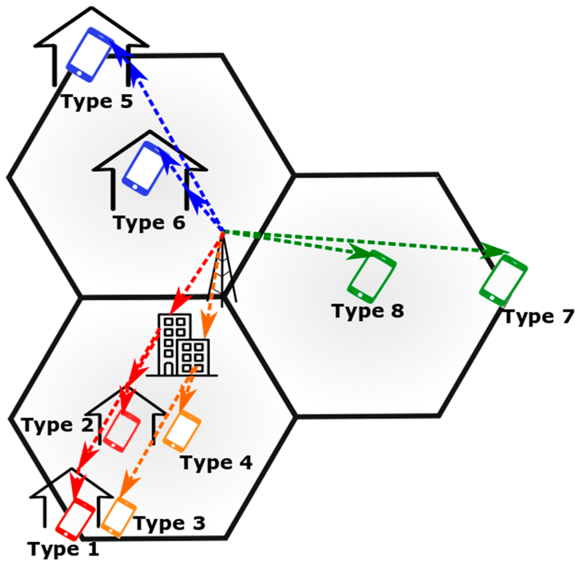
Figure 1 presents the cell layout of analysis model. A hexagonal grid site with three sectors is used [8], and the frequency reuse is assumed to be three. In Figure 1, circles indicate the position of the BS and triangles denote the user positions. It was noted in [3] that the achievable capacity of a user in a building with thick walls or near the edge of a cell should be taken into account. Inspired by this suggestion, we divide the users in one cell into eight different groups to represent different conditions including the combination of LoS or NLoS, indoor or outdoor, and cell center or cell edge in Figure 2. According to the propagation conditions, the user types can be mapped to smart city scenarios. The details of the eight user types are summarized in Table 2. The combination of analysis model and user classification method is designed to reflect the complicated and various possible scenarios in urban environment. The achievable maximum capacity for each user type is quantified as a function of carrier frequency by 3D propagation model [8], and thus the effect of frequency on the spectrum value can be investigated. The 3D propagation model includes such diverse parameters as 3D propagation distance, environment height, standard shadow fading, LOS probability, indoor user rationing, and outdoor-to-indoor penetration loss.

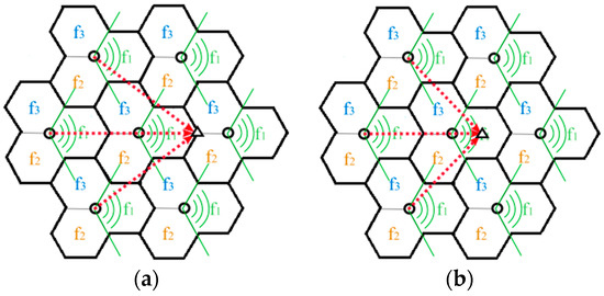
Figure 1. Cell layout (a) user is at cell edge; (b) user at cell center.

Figure 2. Diagram of eight different user types.

Table 2. User conditions and smart city application scenarios for eight different user types in urban environment.

User Type	User Condition	Smart City Application Scenario
Type 1	NLoS + Indoor + Cell Edge	Smart home, Smart office, Shopping mall
Type 2	NLoS + Indoor + Cell center
Type 3	NLoS + Outdoor + Cell Edge	Intelligent vehicle in dense urban, Stadium
Type 4	NLoS + Outdoor + Cell center
Type 5	LoS + Indoor + Cell Edge	Skyscraper
Type 6	LoS + Indoor + Cell center
Type 7	LoS + Outdoor + Cell Edge	Innovative highway transportation
Type 8	LoS + Outdoor + Cell center

Let us describe in more detail the process of quantifying the maximum capacity of each user type. As the dotted line in Figure 1 shows, when only considering the first-tier interference, the user receives interference signals from three adjacent base stations because of the frequency reuse scheme. The maximum user capacity is calculated from the Shannon capacity [17].

$$C=B\times {\log }_2\left(1+SINR\right)$$

(5)

where C is the maximum capacity and B is the bandwidth allocated to each user. Under the assumption that the available bandwidth is 5% of the carrier frequency [14], it is reasonable to consider different bandwidths for different carrier frequencies since much larger available bandwidth is the main motivation for considering the deployment of high frequency bands. The bandwidth allocated to the user is calculated as [14]:

$$B=\frac{5\%\times f_C}{N_{reuse}\times N_{user}}$$

(6)

where $N_{cell}=d_{user}\ast Are{a}_{cell}$, f_C is the carrier frequency, N_reuse is the frequency reuse number, which equals three, N_user is the number of users connected to the BS in one cell, and d_user is the active user density [14]. Area_cell is the area of one cell as follows:

$$Are{a}_{cell}=2.6\times R^2=2.6\times {\left(\frac{ISD}{3}\right)}^2$$

(7)

where R is the cell radius, which equals 1/3 of the inter-site Distance (ISD). Back to Equation (5), SINR can be calculated from Equation (2) and thus is used to calculate P_R and I. Rather than Equation (3), the equation defined in technical report 36.942 for 3GPP [18] is used here:

$$P_R=\{\begin{array}{l}{P}_T-\max \left(L+SF-G_T-G_R,MCL\right)\\ ,\mathrm{outdoor}\mathrm{user}\\ P_T-\max \left(L+SF-G_T-G_R+L_{O2I},MCL\right)\\ ,\mathrm{indoor}\mathrm{user}\end{array}$$

(8)

where P_T is the transmitter power of the BS antenna, G_T is the transmitter antenna gain and G_R is the receiver antenna gain. The path loss L and outdoor to indoor penetration loss L_O2I are calculated from the 3D path loss model and the low-loss out to the indoor penetration model in technical report 38.901 for 3GPP [8], respectively. Please note that the indoor user is standing by the wall or window, so we assume no inside loss after signal penetration through the wall or window. Additionally, SF is shadow fading [8] and MCL is minimum coupling loss [18]. In Figure 1, the interference I in (2) is the sum of the power of three received interference signals transmitted by the adjacent three BSs:

$$I=\{\begin{array}{l}{\displaystyle \sum _1^3\left\{P_T-\max \left(L_i^{\prime }+SF-G_T-G_R,MCL\right)\right\}}\\ ,\mathrm{outdoor}\mathrm{user}\\ {\displaystyle \sum _1^3\left\{P_T-\max \left(L_i^{\prime }+SF-G_T-G_R+L_{O2I},MCL\right)\right\}}\\ ,\mathrm{indoor}\mathrm{user}\end{array}$$

(9)

where $L_i^{\prime }$ is the path loss of the interference signal transmitted by interference BS i and is also calculated with the 3D path loss model. When combining Equations (2) and (5) with different distances between the user and the BS, the maximum achievable capacity for all eight user types can be estimated. Since the 3D propagation model in [8] supports frequency bands ranging from 500 MHz to 100 GHz in urban environments, the spectrum from 500 MHz to 40 GHz is investigated for both UMa and UMi-street canyon scenarios. The parameters used in the analysis for these scenarios are summarized in Table 3. The path loss models for different scenarios and frequency ranges are also summarized in Table 4.

Table 3. Parameters in scenarios [8,14,15,18].

Parameters	UMa	UMi—Street Canyon
TX Antenna Height (m)	25	10
Outdoor user RX antenna height (m)	1.5	1.5
Indoor user RX antenna height (m)	9	9
Inter-site Distance ISD (m)	500	200
TX antenna gain, GT (dBi)	15	15
RX antenna gain, GR (dBi)	0	0
BS TX power, PT (dBm)	46	46
Thermal noise density (dBm/Hz)	−174	−174
Effective environment height (m)	1	1
Active user number (users/km2)	300	300
Minimum coupling loss, MCL (dB)	70	70
Shadow fading in LOS (dB)	4	4
Shadow fading in NLOS (dB)	6	7.82

Table 4. Simulation Parameters.

Environment	Frequency Ranges	Propagation Model
Suburban	500 MHz~1500 MHz	Hata Model
	1500 MHz~3000 MHz	SUI Model
	3000 MHz~11,000 MHz	SUI Model
Urban	500 MHz~40,000 MHz	3D Model (3GPP)

3. Numerical Results

3.1. Suburban Environment

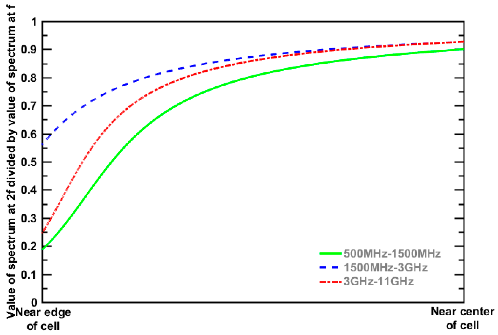
Figure 3 shows the ratio of the data rate at frequency 2f divided by the data rate at frequency f on the y axis versus the spectrum value on the x axis, which is the data rate divided by the bandwidth. These are evaluated for the three frequency bands 500 MHz to 1.5 GHz, 1.5 GHz to 3 GHz, and 3 GHz to 11 GHz. Please note that the spectrum efficiency for each frequency range is normalized to show the same interval on the x axis. Also note that the numerical result for 500 MHz to 1.5 GHz in this paper is almost the same as the results in [3]. In Figure 3, low spectrum efficiency corresponds to the cell edge, but high spectrum efficiency indicates the cell center. At the cell edge, doubling the frequency causes a drop in the data rate of only 20% to 25%, especially for 500 MHz to 1.5 GHz and 3 GHz to 11 GHz. Meanwhile, data rates around 80% to 90% can be achieved by doubling the frequency at the cell center. Therefore, in the suburban environment, high frequencies have a much lower value at the cell edge. However, the high frequency has almost the same impact as the low frequency at the cell center. In conclusion, the result in [3] is confirmed with extensive analysis of the different frequency bands.

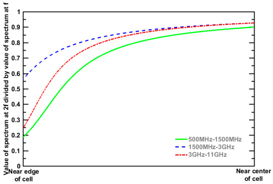
Figure 3. Ratio of the spectrum value at frequency 2f to f in suburban environment.

3.2. Urban Environment

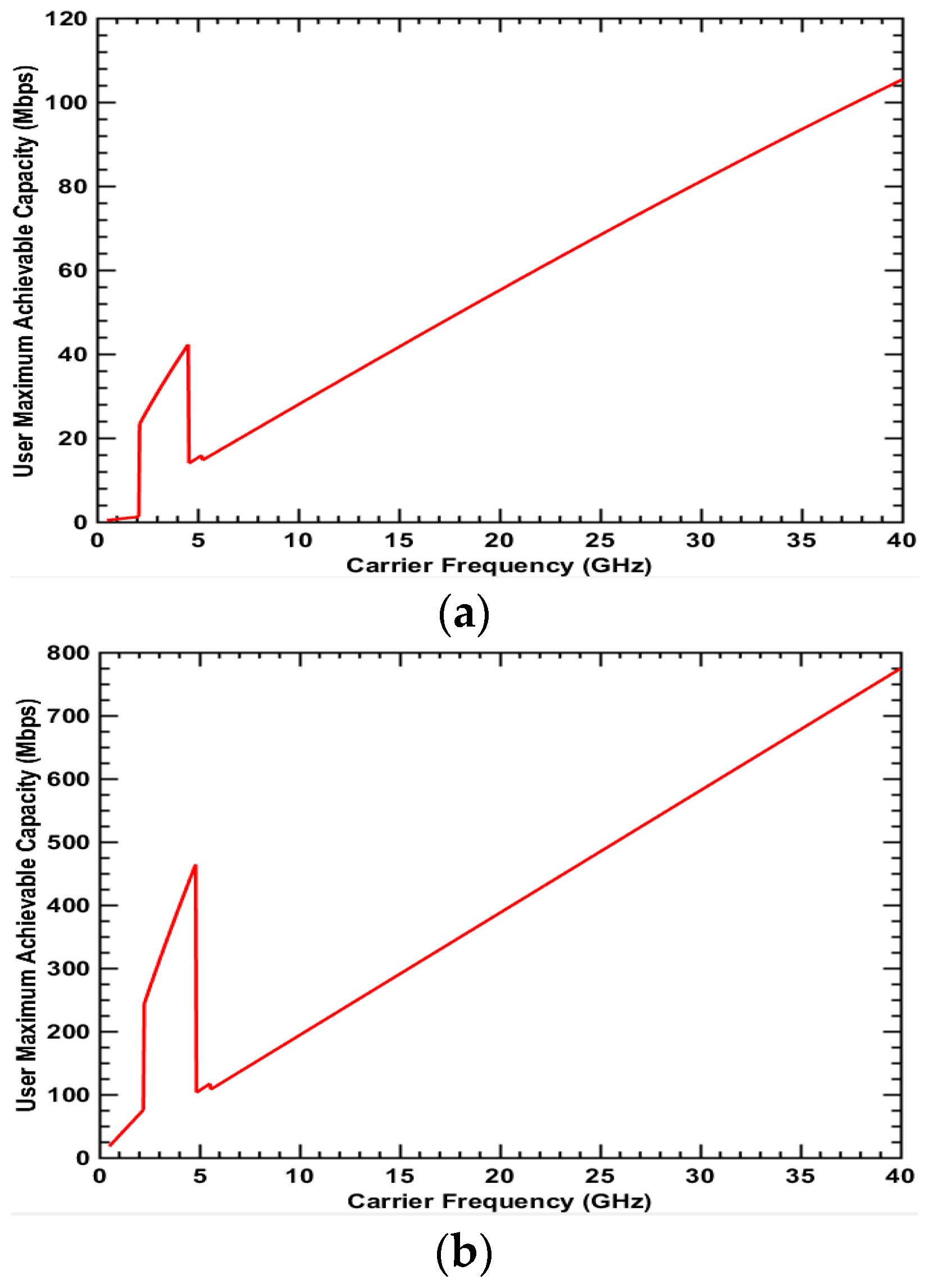
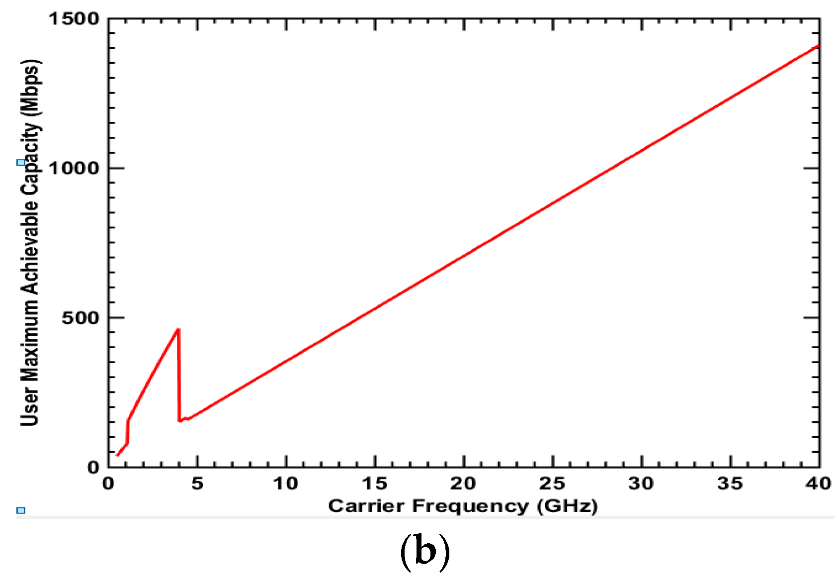
The maximum achievable capacity for eight different user types is estimated and presented in Figure 4, Figure 5, Figure 6, Figure 7, Figure 8, Figure 9, Figure 10 and Figure 11. Additionally, the carrier frequencies that maximize the achievable capacity for 3.5 GHz and 28 GHz are summarized in Table 5. Please note that 3.5 GHz and 28 GHz are considered 5G frequency bands in Korea.

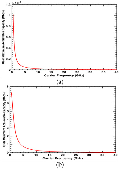
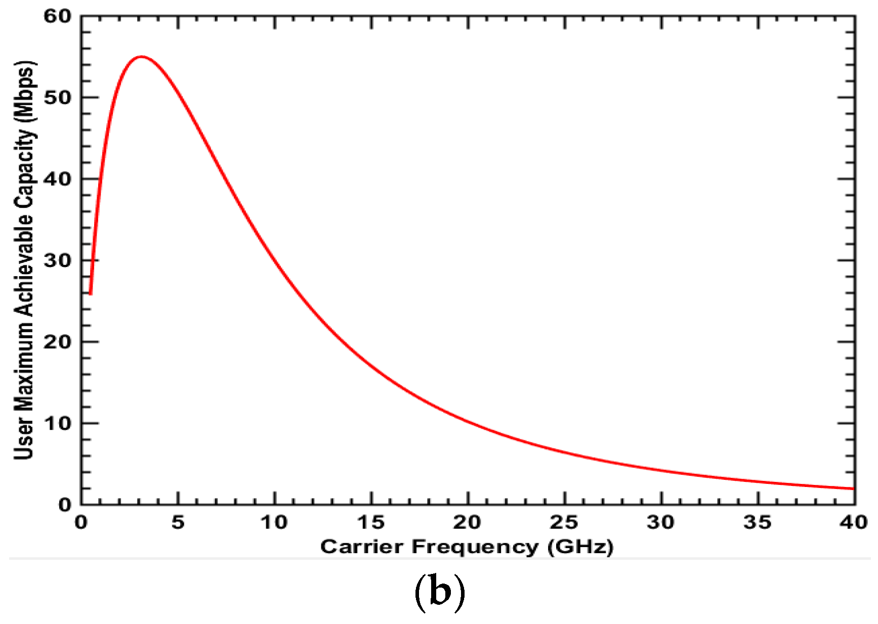
Figure 4. Maximum achievable capacity for Type 1 user: NLOS + Indoor + Cell Edge (a) UMa scenario; (b) UMi-street canyon scenario.

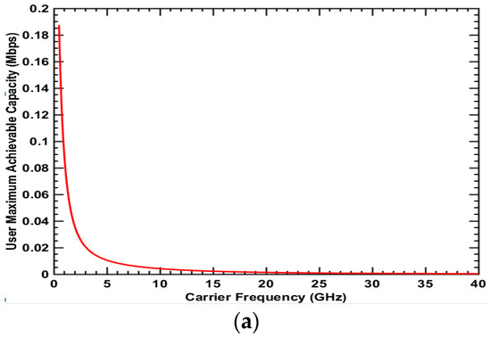
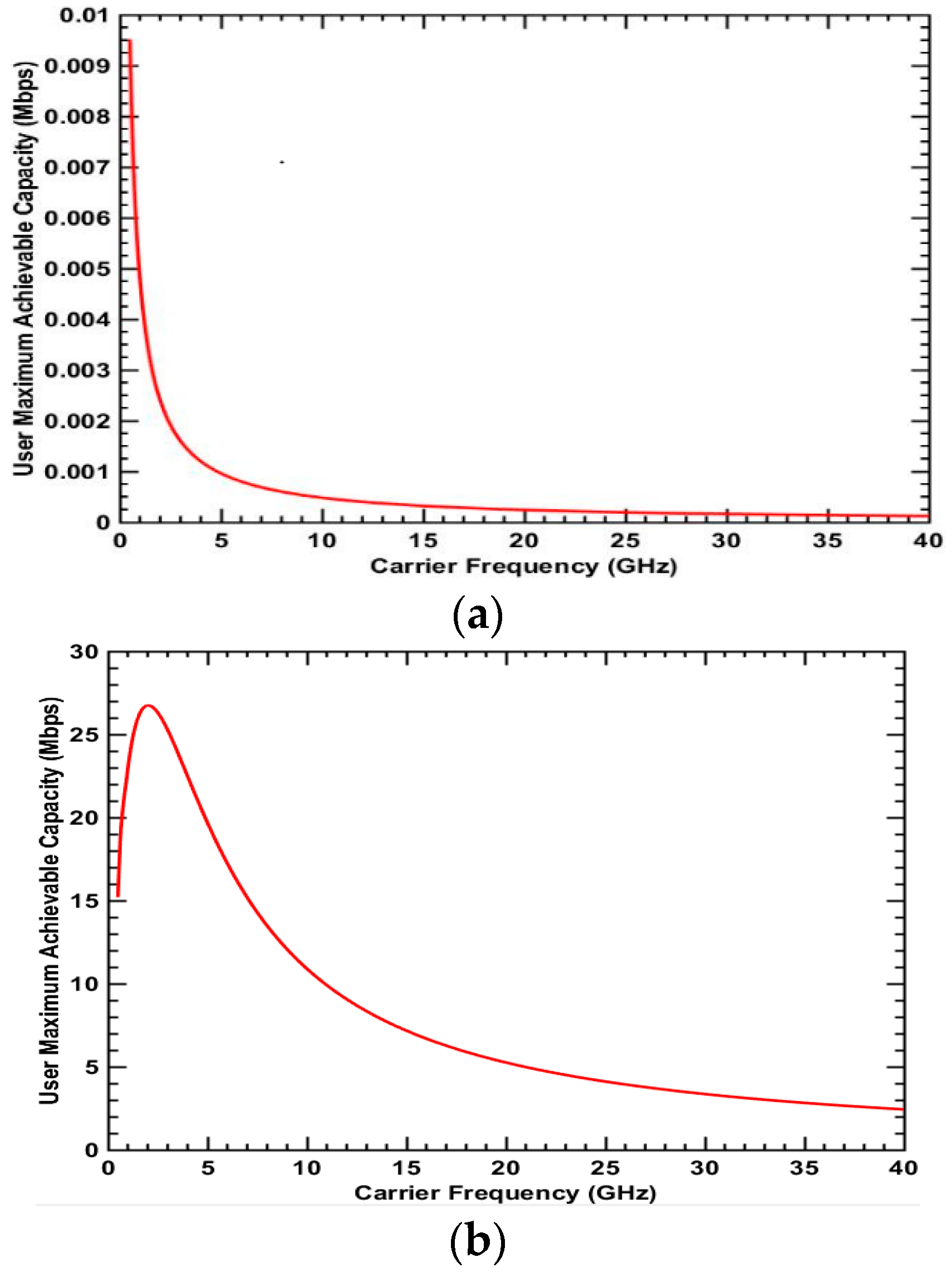
Figure 5. Maximum achievable capacity for Type 2 user: NLOS + Indoor + Cell center (a) UMa scenario; (b) UMi-street canyon scenario.

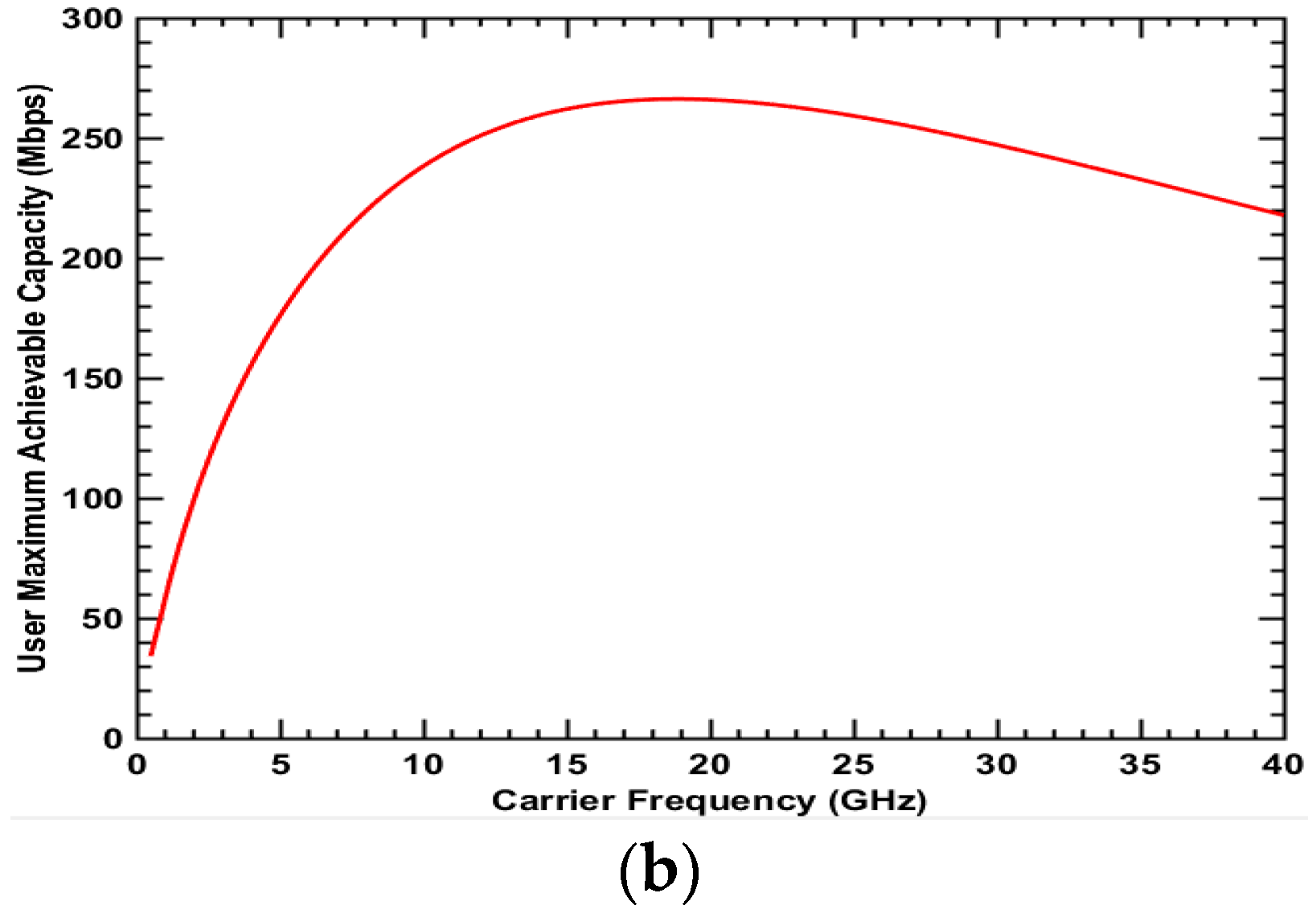
Figure 6. Maximum achievable capacity for Type 3 user: NLOS + Outdoor + Cell Edge (a) UMa scenario; (b) UMi-street canyon scenario.

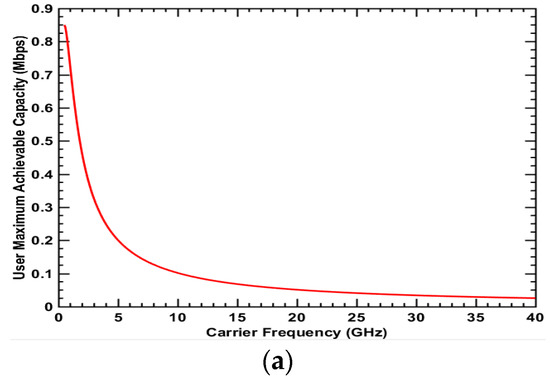
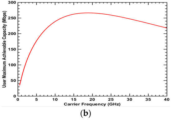
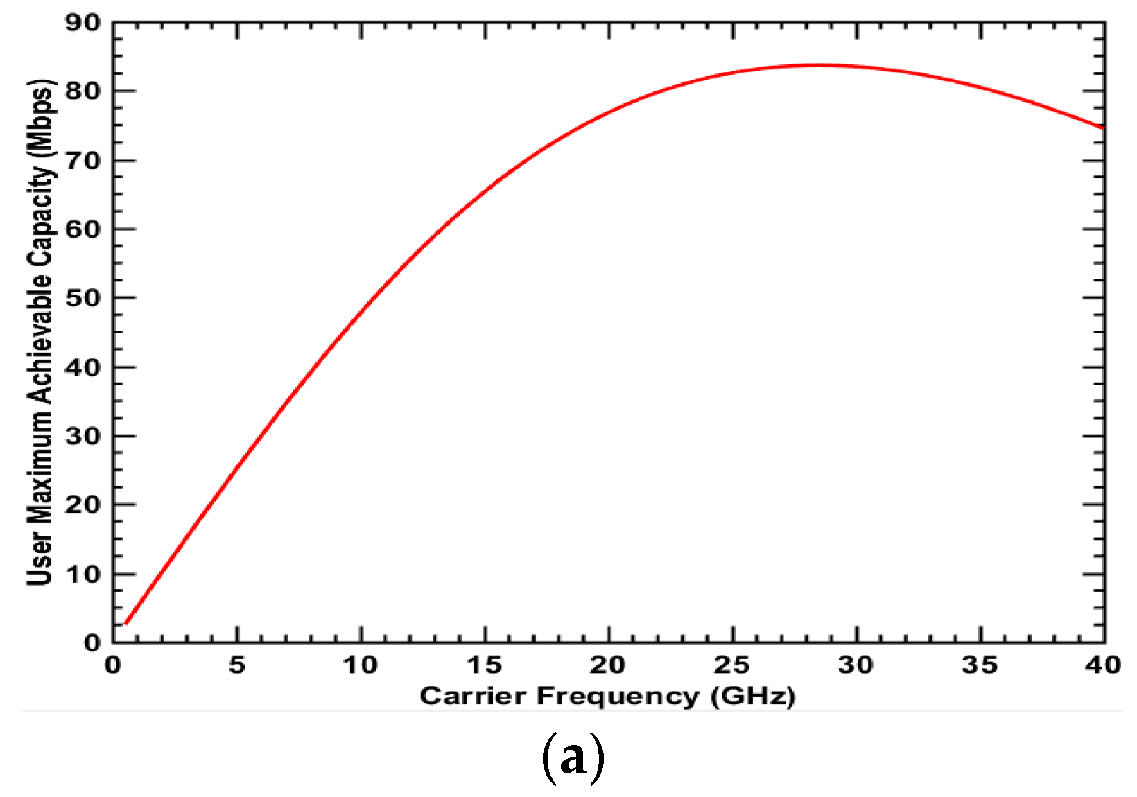
Figure 7. Maximum achievable capacity for Type 4 user: NLOS + Outdoor + Cell center (a) UMa scenario; (b) UMi-street canyon scenario.

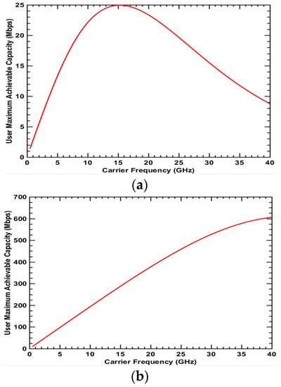
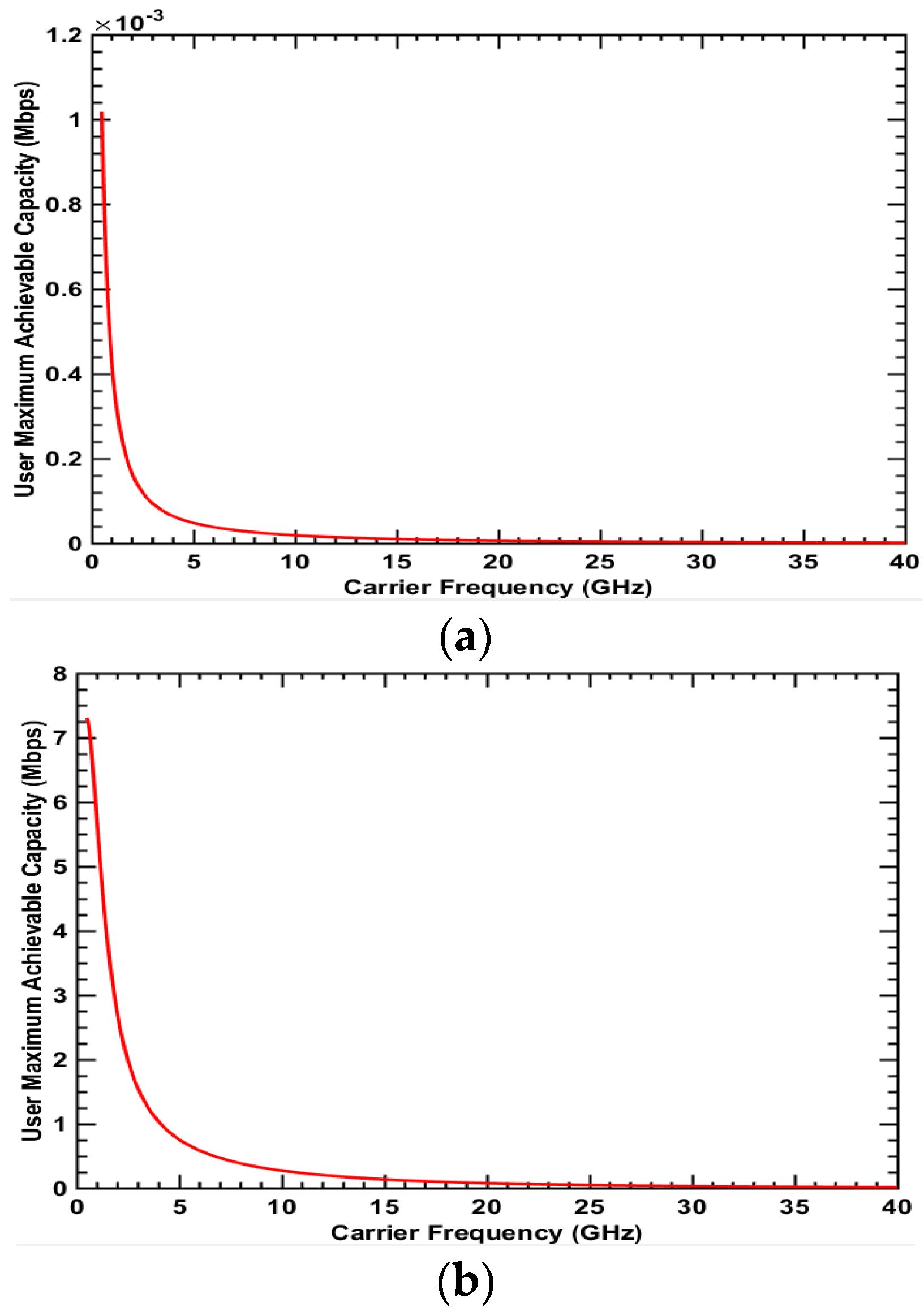
Figure 8. Maximum achievable capacity for Type 5 user: LOS + Indoor + Cell edge (a) UMa scenario; (b) UMi-street canyon scenario.

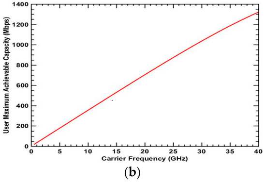
Figure 9. Maximum achievable capacity for Type 6 user: LOS + Indoor + Cell center (a) UMa scenario; (b) UMi-street canyon scenario.

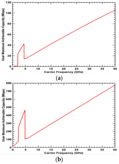
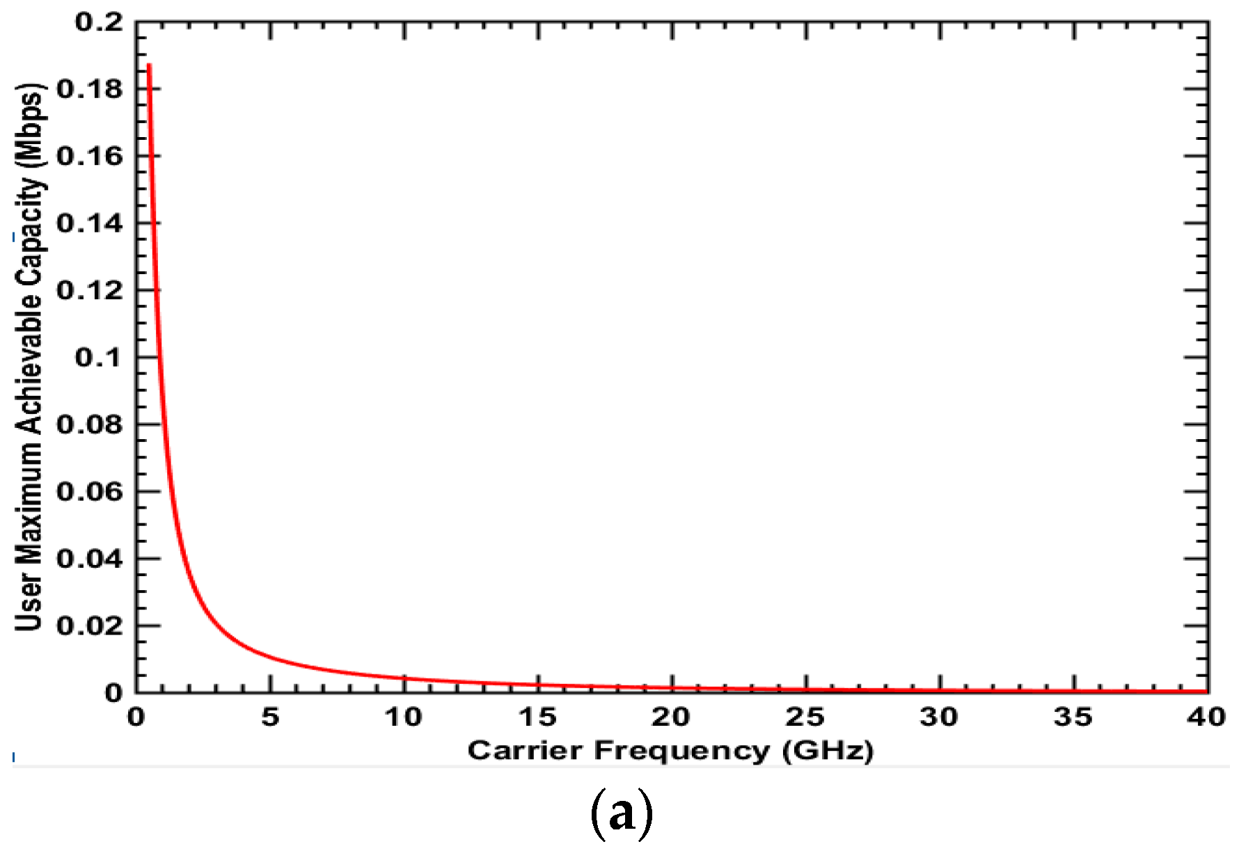
Figure 10. Maximum achievable capacity for Type 7 user: LOS + Outdoor + Cell edge (a) UMa scenario; (b) UMi-street canyon scenario.

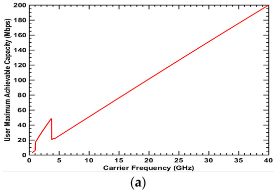
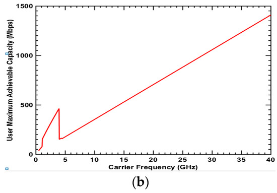
Figure 11. Maximum achievable capacity for Type 8 user: LOS + Outdoor + Cell center (a) UMa scenario; (b) UMi-street canyon scenario.

Table 5. The capacity at 3.5 GHz and 28 GHz, and the frequency with the maximum achievable capacity for each user type in UMa and UMi scenarios.

	UMa				Umi—Street Canyon
User Type	C at 3.5 GHz (Mbps)	C at 28 GHz (Mbps)	fC for Max C(GHz)	Remark*	C at 3.5 GHz (Mbps)	C at 28 GHz (Mbps)	fC for Max C (GHz)	Remark*
Type 1	0.000	0.000	0.5	Lower band	1.24	0.04	0.5	Lower band
Type 2	0.01	0.000	0.5	Lower band	54.70	4.898	3.2	3 GHz
Type 3	0.001	0.000	0.5	Lower band	23.91	3.62	2.0	2 GHz
Type 4	0.28	0.04	0.5	Lower band	193.60	257.25	19.0	19 GHz
Type 5	9.59	17.14	15.1	15 GHz	68.05	501.50	40.0	Higher band
Type 6	27.76	83.65	28.2	28 GHz	124.30	972.00	40.0	Higher band
Type 7	34.65	76.10	40.0	Higher band	355.75	542.50	40.0	Higher band
Type 8	46.17	141.10	40.0	Higher band	414.75	986.50	40.0	Higher band

* “Remark”: the frequency band which has higher or peak spectrum value for each user type.

Figure 4, Figure 5, Figure 6 and Figure 7 show the maximum achievable capacity for user types 1, 2, 3 and 4, respectively. These user types have the NLoS condition in common. Figure 4a, Figure 5a, Figure 6a and Figure 7a for the UMa scenario present similar curve tendencies. Whether at the cell center or cell edge, indoor or outdoor, the achievable capacity decreases dramatically as the frequency increases. This is because the path loss for higher frequencies in the NLoS condition is more severe and thus the advantage of wider bandwidth for higher frequency cannot be reflected. As discussed previously, the spectrum value in the urban scenario is investigated in term of the achievable user capacity. Therefore, in the NLoS condition for the urban environment, the lower frequency has a higher spectrum value and thus will be the better choice for deployment. In Figure 4b, Figure 5b, Figure 6b and Figure 7b for the UMi-street canyon scenario where the BS antenna height is lower in comparison to Uma, the maximum achievable capacity is high compared to the UMa scenario. This is because the ISD in the UMi-street canyon scenario is 200 m, which is much smaller than 500 m in the UMa scenario. This results in smaller path loss. For user types 2, 3 and 4, the curve tendency is different from the UMa scenario. The achievable capacity for the user first increases as the frequency increases and reaches a peak value around 3.2 GHz in Figure 5b, 2 GHz in Figure 6b and 19 GHz in Figure 7b, respectively. The reason the peak exists is that there is a trade-off between bandwidth and path loss. Before the peak value, the wider bandwidth for higher frequency can increase the capacity, compensating for higher path loss and penetration loss. However, as the frequency increases beyond the peak point, the benefits of the wider bandwidth decrease gradually due to dramatically higher path loss and penetration loss. Therefore, in the UMi-street canyon scenario, the medium frequency has the highest spectrum value in the NLoS condition.

The maximum achievable capacities for the remaining user types 5, 6, 7, and 8 are presented in Figure 8, Figure 9, Figure 10 and Figure 11, respectively. These user types have the LoS condition in common. In Figure 8a and Figure 9a, the curve tendencies in the UMa scenario are similar but differ from tendency in the previous figures. Firstly, the maximum achievable capacity increases and then decreases as the frequency increases. It reaches the peak point at a frequency of 15 GHz in Figure 8a and 28 GHz in Figure 9a. For LoS and indoor conditions like an office building or a large supermarket, the medium frequency may have the highest spectrum value and be the better choice. The curve tendencies in Figure 10 and Figure 11 are similar. The user types for these two figures are in LoS and outdoor conditions without penetration loss and with lower path loss. Furthermore, the wider bandwidth at higher frequencies is enough to show high achievable capacity. Therefore, the maximum achievable capacity keeps increasing as the frequency increases. Please note that the abrupt change in the curves is a result of the distance between BS and MS reaching the break point in the 3GPP 3D path loss model. The results indicate that higher frequency is better than lower frequency and would be a better choice for the carrier to deploy services in LoS and outdoor conditions such as in a large stadium.

From the previous figures, it is obvious that three user conditions, namely NLoS or LoS, indoor or outdoor, and cell edge or cell center, impact the spectrum value in urban areas. Here, a general analysis will be performed. Firstly, we can compare Figure 4, Figure 5, Figure 6 and Figure 7 with Figure 8, Figure 9, Figure 10 and Figure 11. The curve is generally decreasing in Figure 4, Figure 5, Figure 6 and Figure 7, which have the NLoS condition in common. However, the curve is convex or increasing in Figure 8, Figure 9, Figure 10 and Figure 11, which have the LoS condition in common. Therefore, we can say that NLoS and LoS are the key factors that influence the spectrum value at different frequencies. Secondly, more specifically, we may compare Figure 8a and Figure 9a with Figure 10a and Figure 11a. The curves in Figure 8a and Figure 9a, which are both from indoor conditions, are generally convex. However, the curve changes to an incline in Figure 10a and Figure 11a, which are from outdoor conditions. Therefore, the graphs show that the location of the user indoor or outdoor is more important than whether the user is located at the cell center or edge. In conclusion, when carriers consider the spectrum values at different frequencies, NLoS and LoS should be the primary consideration and indoor and outdoor conditions should be secondary.

Table 5 shows the capacity at 3.5 GHz and 28 GHz, and the frequency with the maximum achievable capacity for each user type in UMa and UMi scenarios. It is interesting to search for the optimal frequency, which gives the peak achievable user capacity. In the UMa scenario, 28 GHz for user type 6 provides the highest value of 85 Mbps. In the UMi-street canyon scenario, 3.2 GHz for user type 2 provides the highest value of 55 Mbps, and 2 GHz for user type 3 provides the highest value of 26 Mbps. If we consider 3.5 GHz and 28 GHz as candidate frequency bands in Korea, 28 GHz may be the best choice for LOS and indoor conditions in the UMa scenario and 3.5 GHz can be employed in the UMi-street canyon scenario. In the UMa scenario in Table 5, the achievable capacities for user types in the NLOS condition are all close to zero. When comparing the UMa scenario with the UMi-street canyon scenario, the maximum achievable capacities for all user types are much higher in the UMi-street canyon scenario, especially for higher frequencies. This is because the BS antenna height in the UMi–street canyon scenario is 15 m lower than that in the UMa scenario. In the 3D propagation model with the same horizontal distance between the BS and user equipment (UE), a higher antenna can lead to a longer propagation distance. That is, the BS antenna is much closer to users in the UMi–street canyon scenario. Therefore, the UMi-street canyon deployment scenario is efficient and more suitable for high frequency band deployment.

4. Conclusions

In this paper, the spectrum value is analyzed in suburban and urban environments. In the suburban environment, lower frequencies seem more valuable at the cell edge. Meanwhile, high frequencies have almost the same impact as low frequencies at the cell center. In the urban environment, the spectrum value depends on the area of the cell and the user conditions. In the NLoS condition, a lower frequency shows a higher spectrum value. For LoS with indoor conditions, medium frequency bands are the best choice, and for LoS with outdoor dominant conditions, high-frequency bands are more beneficial. Additionally, 3.5 GHz may show high values in NLoS and indoor conditions in the UMi deployment scenario. Furthermore, 28 GHz may be the optimal choice for LoS and indoor conditions in the UMa deployment scenario. In conclusion, NLoS or LoS is the primary consideration, and indoor or outdoor is the secondary. In addition, UMi deployment with lower antenna heights is more efficient in urban scenarios. Please note that the conventional SISO antenna is considered in this work. The employment of advanced technologies like (Massive) MIMO antenna can affect the spectrum value. Additionally, single frequency network (SFN) deployment may give an impact on the spectrum values. This paper can suggest a bound of the spectrum value for readers’ information. The consideration on MIMO and SFN will be our future work.

References

- Lutilsky, D.; Mazor, K. Theoretical approaches for spectrum pricing. In Proceedings of the 2015 57th International Symposium ELMAR, Zadar, Croatia, 28–30 September 2015; pp. 57–60. [Google Scholar]
- Malisuwan, S.; Kaewphanuekrungsi, W.; Milindavanij, D. Mobile spectrum value and reserve price by using benchmarking approaches. Int. J. Sci. Eng. Technol. 2016, 5, 81–84. [Google Scholar]
- Peha, J.M. Cellular Competition and the Weighted Spectrum Screen. In Proceedings of the TPRC 41: The 41st Research Conference on Communication, Information and Internet Policy, Arlington, VA, USA, 27–29 September 2013. [Google Scholar]
- Bazelon, C.; McHenry, G. Spectrum value. Telecommun. Policy 2013, 37, 737–747. [Google Scholar] [CrossRef]
- Li, Q.C.; Niu, H.; Papathanassiou, A.T.; Wu, G. 5G network capacity: Key elements and technologies. IEEE Veh. Technol. Mag. 2014, 9, 71–78. [Google Scholar] [CrossRef]
- Abhayawardhana, V.; Wassell, I.; Crosby, D.; Sellars, M.; Brown, M. Comparison of empirical propagation path loss models for fixed wireless access systems. In Proceedings of the 2005 IEEE 61st Vehicular Technology Conference, Stockholm, Sweden, 30 May–1 June 2005; Volume 1, pp. 73–77. [Google Scholar]
- Hata, M. Empirical formula for propagation loss in land mobile radio services. IEEE Trans. Veh. Technol. 1980, 29, 317–325. [Google Scholar] [CrossRef]
- 3GPP. Study on Channel Model for Frequencies from 0.5 to 100 GHz (Release 14); 3GPP: Valbonne, France, 2017. [Google Scholar]
- Wei, Y.; Hwang, S. Investigation of spectrum values in rural environments. ICT Express 2018, in press. [Google Scholar] [CrossRef]
- Matheson, R.; Morris, A.C. The technical basis for spectrum rights: Policies to enhance market efficiency. Telecommun. Policy 2012, 36, 783–792. [Google Scholar] [CrossRef]
- Lamas, S.R.; Gonzalez, D.; Hamalainen, J. Indoor planning optimization of ultra-dense cellular networks at high carrier frequencies. In Proceedings of the Wireless Communications and Networking Conference Workshops (WCNCW), New Orleans, LA, USA, 9–12 March 2015; pp. 23–28. [Google Scholar]
- Osseiran, A.; Monserrat, J.F.; Marsch, P. (Eds.) 5G Mobile and Wireless Communications Technology; Cambridge University Press: Cambridge, UK, 2016. [Google Scholar]
- Afrić, W.; Pilinsky, S.Z. UMTS LTE downlink cell size calculation. In Proceedings of the ELMAR-2012, Zadar, Croatia, 12–14 September 2012; pp. 105–108. [Google Scholar]
- López-Pérez, D.; Ding, M.; Claussen, H.; Jafari, A.H. Towards 1 Gbps/UE in cellular systems: Understanding ultra-dense small cell deployments. IEEE Commun. Surv. Tutor. 2015, 17, 2078–2101. [Google Scholar] [CrossRef]
- 3GPP. Evolved Universal Terrestrial Radio Access (E-UTRA); Radio Frequency (RF) Requirements for LTE Pico Node B (Release 14); 3GPP: Valbonne, France, 2017. [Google Scholar]
- Holma, H.; Toskala, A. WCDMA for UMTS: HSPA Evolution and LTE; John Wiley & Sons: Hoboken, NJ, USA, 2007. [Google Scholar]
- Jing, S.; Tse, D.N.; Soriaga, J.B.; Hou, J.; Smee, J.E.; Padovani, R. Multicell downlink capacity with coordinated processing. EURASIP J. Wirel. Commun. Netw. 2008, 2008, 18. [Google Scholar] [CrossRef]
- 3GPP. Evolved Universal Terrestrial Radio Access (E-UTRA); Radio Frequency (RF) System Scenarios (Release 14); 3GPP: Valbonne, France, 2017. [Google Scholar]
© 2018 by the authors. Licensee MDPI, Basel, Switzerland. This article is an open access article distributed under the terms and conditions of the Creative Commons Attribution (CC BY) license (http://creativecommons.org/licenses/by/4.0/).