1. Introduction
Home Energy Management Systems (HEMS) are used to manage energy consumption in the home, for example, by scheduling the load operation time, managing renewable energy resources, and providing battery storage [
1]. The system integrates electronic sensors, intelligent controllers, wireless communications, and smart load switches. To provide optimal energy consumption, a residential demand response (DR) program, consisting of the following attributes can be employed [
1]: (a) real-time pricing, as electricity price varies over the day and month; (b) time of use pricing as the electricity price varies between peak and off-peak hours; (c) critical peak pricing as the electricity price changes within a short period; (d) direct load program as the electricity price can change at any time from the utility side; (e) curtailable program as the electricity price changes during emergencies; and (f) demand bidding where the electricity price depends on the customer’s bid.
The DR algorithm in a HEMS is usually employed to minimize the cost of electricity consumption [
2]. In individual homes, the DR method controls the load and energy resources using optimization techniques, such as the Genetic Algorithm (GA) and Mixed Integer Linear Programming (MILP). In community or groups of homes, a Community Energy Management System (CEMS) is used to manage the power in order to minimize the electricity cost of a group of homes.
Typical HEMS consist of sensing devices (current, voltage, temperature, light sensors); measuring devices (electricity, gas, water meters); smart appliances (home appliances that can be monitored and controlled remotely); wireless communication (WiFi, Zigbee, Z-wave) and an energy management system (informative, automated, advanced function, integrated system) [
3]. Even though HEMS offer promising benefits, their implementation faces challenging issues such as the expensive costs of the devices and installation; the lack of HEMS standards; low awareness of the customers; the problems involved in creating larger systems; the choice of communication technology; and a requirements of intelligent systems [
3].
Many algorithms and systems have been developed to implement HEMS [
4,
5,
6,
7,
8,
9,
10,
11,
12,
13,
14,
15,
16,
17,
18,
19,
20,
21,
22]. A HEMS which is used to reduce the electricity cost while maintaining the Quality of Experience (QoE) of the users was proposed in Ref. [
4]. The method consists of two algorithms: the QoE-aware Cost Saving Scheduling (Q-CSAS) that schedules loads according to user habits and time-of-usage tariffs, and the QoE-aware Renewable Source Power Allocation (Q-RSPA) that schedules the loads when there is a surplus of energy from renewable energy resources.
Mixed Integer Linear Programming (MILP) was employed to solve the optimization problem in the HEMS proposed in Ref. [
5]. The method optimizes the electricity cost by load shifting and renewable energy sharing. Mixed Integer Non-Linear Programming (MINLP) was employed in Ref. [
6]. The authors in Ref. [
6] proposed a multi-objective MINLP to find the optimal energy use in a home with three dependent objectives: (a) minimization of the operation cost, (b) maximization of the user’s convenience level; and (c) maximization of the thermal comfort level.
The authors in Ref. [
7] proposed an energy management system for scheduling home appliances using a single knapsack method. The system consists of an energy management center (EMC) that monitors and controls the energy wirelessly, a load scheduler that schedules the loads on a day ahead tariff basis, and a human machine interface (HMI) that provides an interface between the home appliances and the EMC. The HMI communicates with the appliances using a ZigBee module.
The authors in [
8] proposed a HEMS algorithm to limit the power consumption of home appliances while keeping a comfortable level based on priority. The system deals with power-intensive loads such as water heaters, clothes dryers, air conditioners, and electric vehicles. The simulation of a decision control strategy was implemented using C++ language [
9]. The hardware demonstration of the HEMS was implemented on the embedded personal computer (PC), the load controller, and the ZigBee communication module [
9]. The performance of the HEMS and the communication delay were evaluated [
9]. The Zigbee modules were employed in the energy saving system in a home heating plant [
10]. The system consists of temperature sensors and actuators which send the data to a central unit using Zigbee communication. The method employs a simple control algorithm to control the water valve of the heating system based on the room temperature.
Our previous work [
11] implemented a HEMS on an embedded platform. The HEMS architecture consisted of load and smart controllers. The load controllers were implemented on Arduino microcontrollers, while the smart controller was implemented on a Raspberry Pi module. The load controllers and the smart controller communicate using the ZigBee wireless module. The MILP method was employed to minimize the peak power of load consumption. The method was implemented on the Raspberry Pi using C++ language. In our study [
11], the MILP execution time and the data transmission time from the local controllers to the smart controller were examined.
An intelligent cloud-based HEMS (CHEMS) was proposed in [
12]. The CHEMS consists of an intelligent cloud-based management server (iCMS) and an intelligent cloud-based metering device (iCMD). The iCMS consists of an application layer (service manager, consumer profile), a management layer (pattern manager, service scheduler) and a cloud infrastructure layer (virtual machine monitor). The iCMD consists of an application layer (electricity measurement, communication, remote control), an adaptive configuration layer (application manager, dynamic reconfiguration rules) and a hardware management layer (power management, device driver, OS kernel).
HEMS based on fuzzy logic controllers (FLCs) (FLC-based HEMS) were proposed in Refs. [
13,
14,
15,
16,
17,
18,
19,
20,
21,
22]. The works are summarized in
Table 1, where the input and output variables of the FLC, the objective function, and the implementation platform are presented. The advantages of using the FLC are (a) it solves the difficulties of classical optimization problems; and (b) it is computationally efficient and thus suitable for embedded applications. The table shows that there is no general approach to the FLC-based HEMS. The FLC is designed according to the particular condition, where the variables, membership functions, and the inference rules should be defined accordingly.
A major problem in developing the FLC is determining the fuzzy membership functions and the fuzzy rules that match the desired objective. Several methods, such as the GA [
22,
23,
24,
25], particle swarm optimization (PSO) [
26], ant colony optimization (ACO) [
27], and bee colony optimization (BCO) have been proposed to tune the fuzzy memberships and the fuzzy rules. In Ref. [
22], the GA was employed for online tuning of the fuzzy rules and the membership functions. Offline tuning of the fuzzy membership functions was proposed in Ref. [
23]. In Ref. [
24], the fuzzy membership functions, fuzzy rules, and scaling gains were encoded to the 44-bits of the GA-chromosome for automated tuning. To tune the complex parameters of the FLC, the hierarchical GA was proposed in Ref. [
25]. In this method, the input variables and delays were treated in the first level. The membership functions were treated in the second level. The third level treated the individual rules. The set of fuzzy rules were treated in the fourth level. Finally, the fifth level treated the whole FLC system.
In Ref. [
26], the PSO was used to optimize ten parameters which represented the fuzzy membership functions of the FLC. The integral of time-weighted-squared-error was employed as the fitness function to evaluate the PSO algorithm. In Ref. [
27], the type of fuzzy membership functions, the parameters of the fuzzy membership functions, and the fuzzy rules were optimized using the ACO. The ACO was executed sequentially and hierarchically, i.e., it first optimized the type of fuzzy membership functions, then the parameters of the fuzzy membership function, and finally, the fuzzy rules. In Ref. [
28], the BCO was employed to optimize the scale factors, the fuzzy membership functions, and the fuzzy rules of the FLC. The works in Refs. [
22,
23,
24,
25,
26,
27,
28] showed that by optimizing or tuning the fuzzy parameters of the FLC automatically, its performance was better than the manually tuned FLC.
This paper deals with the FLC-based HEMS, which is the hardware implementation of our previous work in Ref. [
21]. The objective of the proposed FLC-based HEMS is to minimize the electricity cost in the grid connected PV-battery system. The proposed system is the simple case of the HEMS and does not consider the comfort level, as described in Refs. [
4,
5,
6] yet. However, our work aims to examine the reliability of the low cost hardware implementation of the HEMS, more specifically, the FLC algorithm, on the embedded platform (the WeMos module) [
29].
The FLC is used to switch on/off the loads according to the condition of the PV power, the SOC of the battery, and the total load demand. Instead of using the centralized scheme, our method adopts the distributed FLC in which each load has its own FLC. The proposed distributed FLC offers some benefits as follows. The FLC algorithm is suitable for implementation on the embedded microcontroller due to its simple mathematic operations. However, the microcontroller memory and the execution time will increase when the numbers of the fuzzy membership functions and the rules increase. In the case of FLC-based HEMS, the complexity of the membership functions and the rules depend on the optimization objective and the number of the loads. In the centralized approach, the FLC is implemented on the central unit which requires a fast processor with a large memory. It cannot be implemented easily on the low-cost embedded microcontroller. Our method overcomes this drawback by distributing the FLC on each node (load). Since the load has its own FLC, the number of membership functions and rules are minimized, i.e., only those required to control the particular load are used, allowing the FLC to be easily run on the low-cost embedded microcontroller (WeMos module).
The WeMos module is a WiFi-enabled microcontroller on the Arduino board WiFi communication is employed to exchange tdata between the loads, the PV-battery, and the grid. In this work, we only focus on the implementation of FLC on the embedded system and examine the wireless communication issues of the WiFi module. The implementation of sensors and relays of the load controller is outside the scope of our current work. The main contribution of our work is the implementation of distributed FLC-based HEMS using a low-cost, wireless, embedded platform. Further, automatic tuning of the fuzzy membership function tuning using the Genetic Algorithm (GA) is also developed.
The rest of paper is organized as follows:
Section 2 describes our proposed system. The experimental results and discussion are presented in
Section 3. The conclusions are presented in
Section 4.
2. Proposed System
2.1. Architecture of Electrical System
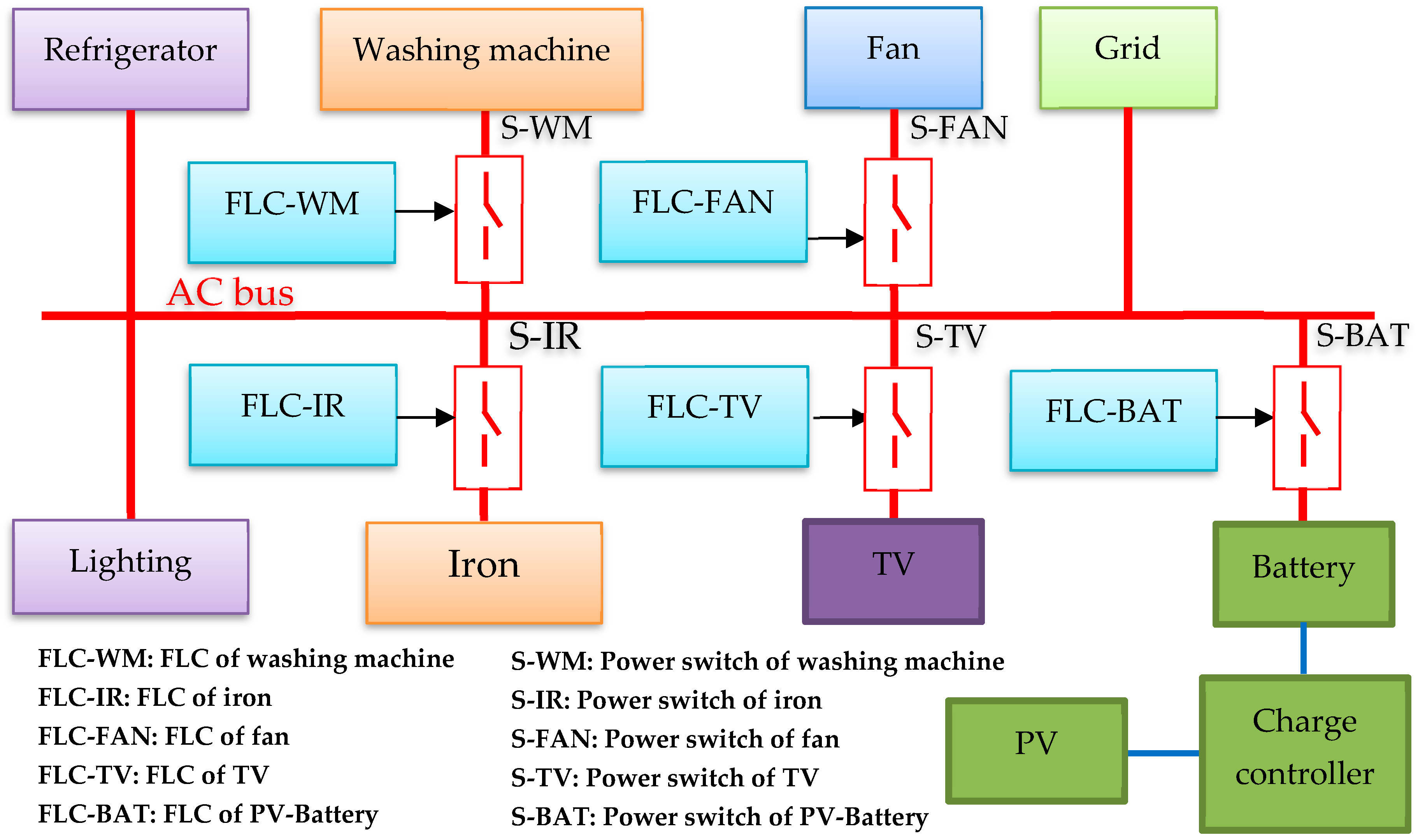
The architecture of the electrical system is depicted in
Figure 1. As shown in the figure, the energy resources consist of the utility grid and the PV-battery system. The PV-battery system is connected to the grid using the grid-tie inverter. It is assumed that the grid is the main electrical resource that is always connected to the AC bus. The PV-battery system delivers the energy to the grid when its required conditions are satisfied. The PV-battery system adopted here is the cascade method in which the PV is connected to the battery using a charge controller. Then, the battery is connected to the grid via a grid-tie inverter.
The objective of our proposed system is to minimize the electricity cost by managing the energy flow from the battery to the loads. Since the battery power depends on the availability of solar energy, the energy usage by the loads should be managed properly. Therefore, an intelligent system, the FLC, was employed. In this work, only six home appliances were considered. However, the approach could be extended to other complex home appliances. The six home appliances were divided into four categories:
Non-shiftable loads: lighting and refrigerator;
Time shiftable loads: washing machine and iron;
Power shiftable load: fan,
Non-essential load: TV.
As discussed previously, the objective of this system is to manage the loads that require energy from the PV-battery system; thus, it is a load scheduling problem. Since the non-shiftable loads cannot be scheduled, they are uncontrolled, and are thus directed to the grid, as shown in the figure. The method shifts the operation time of the time shiftable loads, the power shiftable load and the non-essential load. For the power shiftable load, i.e., the fan, the power supply is varied according to the energy availability from the PV-battery system. Further, the non-essential load is switched on whenever there is excess power.
As shown in the figure, there are five FLC modules that control the power switches. The FLC is implemented on the embedded microcontroller equipped with the WiFi module to communicate with the other FLC modules. Since the FLC is distributed to each load, there is no master control. However, the data required by the FLC is collected from all loads and the PV-battery system using wireless communication, as described in the next section.
2.2. Fuzzy Logic Controller (FLC)
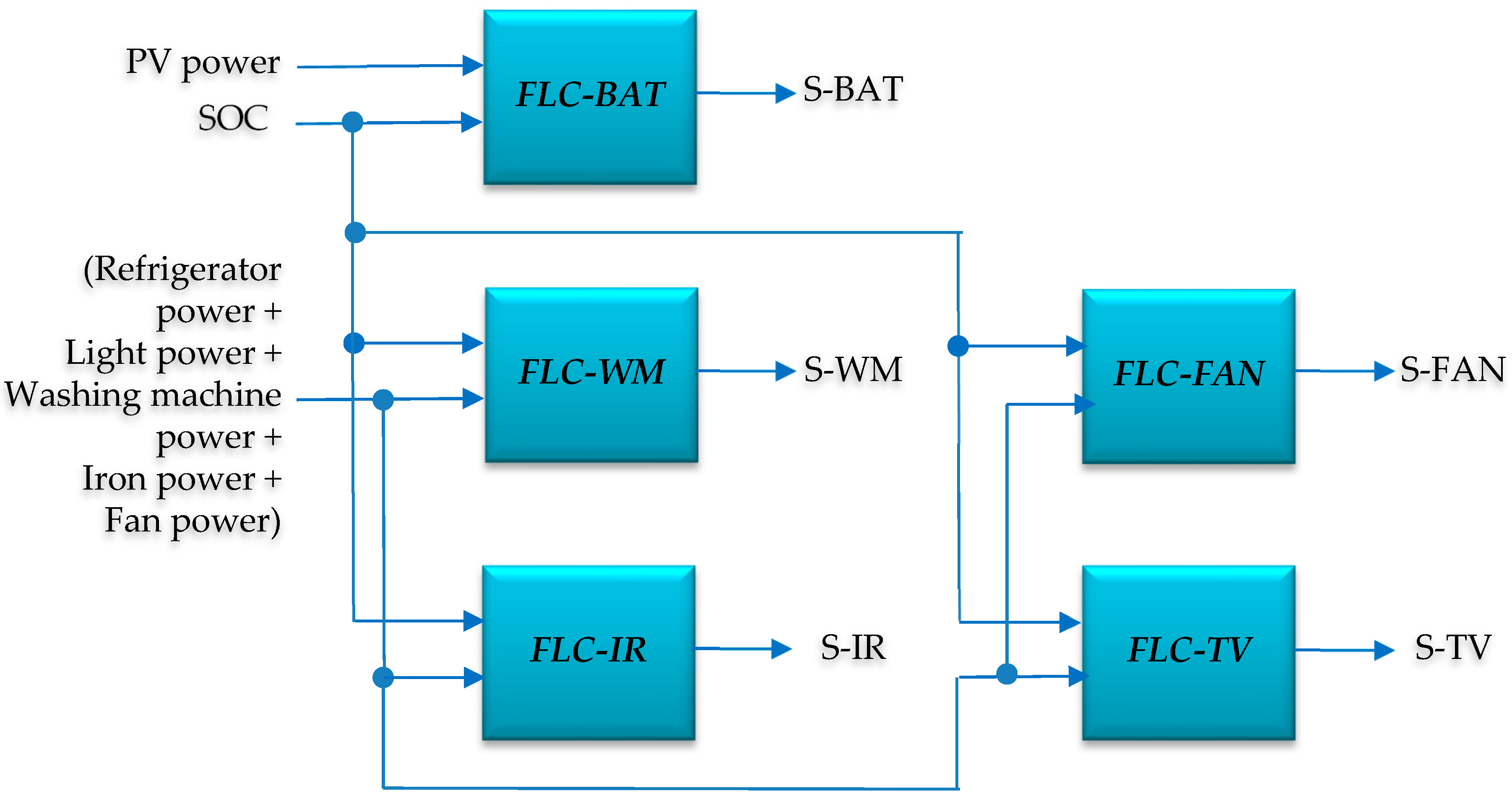
The architecture of proposed FLC is depicted in
Figure 2. The main idea is that the controlled loads should be switched on when there is enough battery power (SOC of battery is high). Meanwhile, the total load power should be low. The latter condition is used to ensure that the battery does not discharge rapidly. As shown in the figure, the input variables of FLC-WM, FLC-IR, FLC-FAN, and FLC-TV are the same, i.e., the SOC of the battery and the total power of the refrigerator, lighting, washing machine, iron, and fan, while the output variable is the respective power switch. The FLC-BAT is developed differently. Its input variables are the SOC of the battery and the PV power, while its output variable is the power switch of the battery (S-BAT). It is noted that the FLCs on the loads are executed when the S-BAT is switch on. All FLCs employ Mamdani-type fuzzy inference.
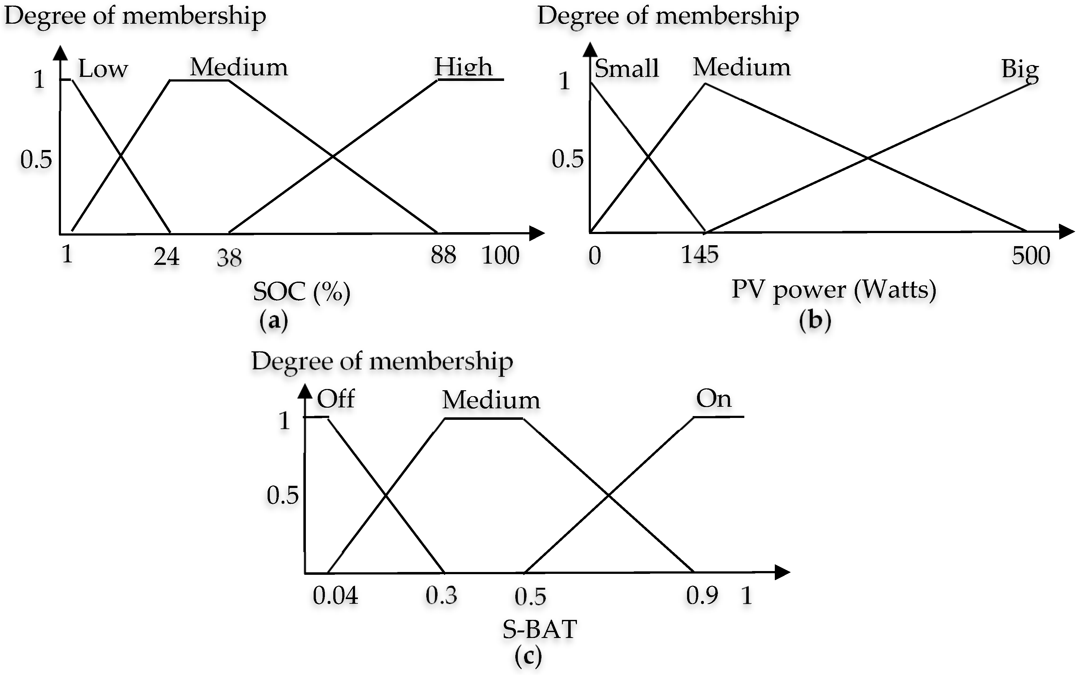
2.2.1. Fuzzy Membership Functions
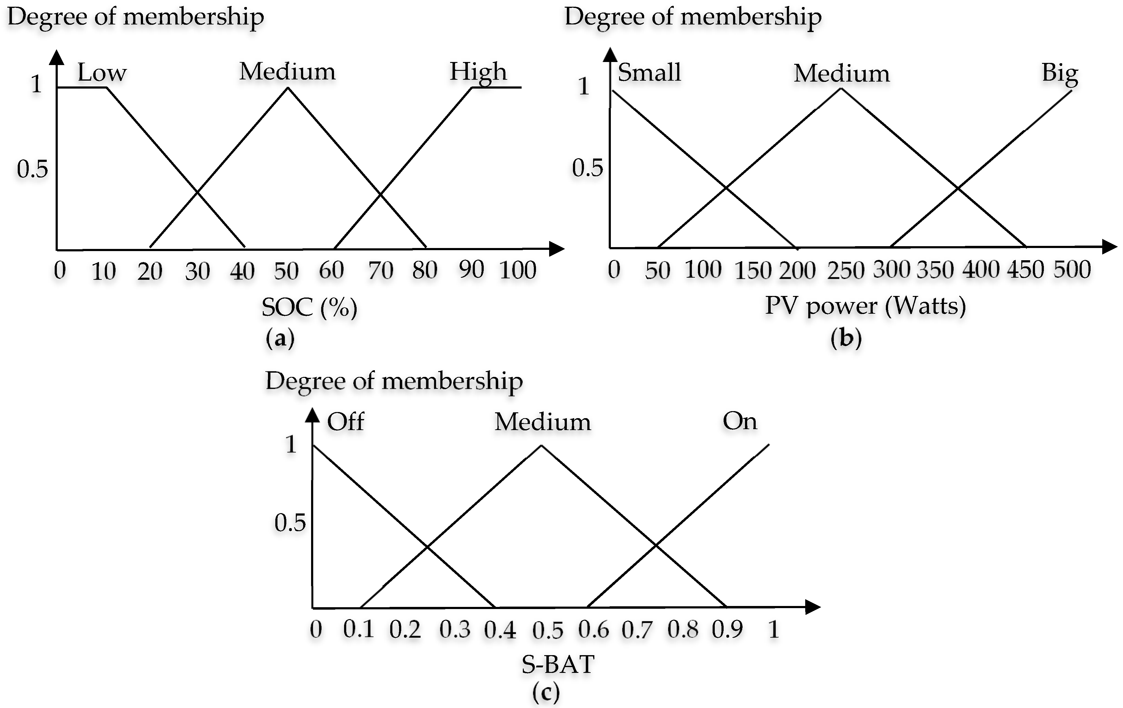
The fuzzy membership functions for the FLC-BAT for the SOC, the PV power, and the S-BAT are shown in
Figure 3a–c, respectively. The membership function of the SOC is applied for all FLCs.
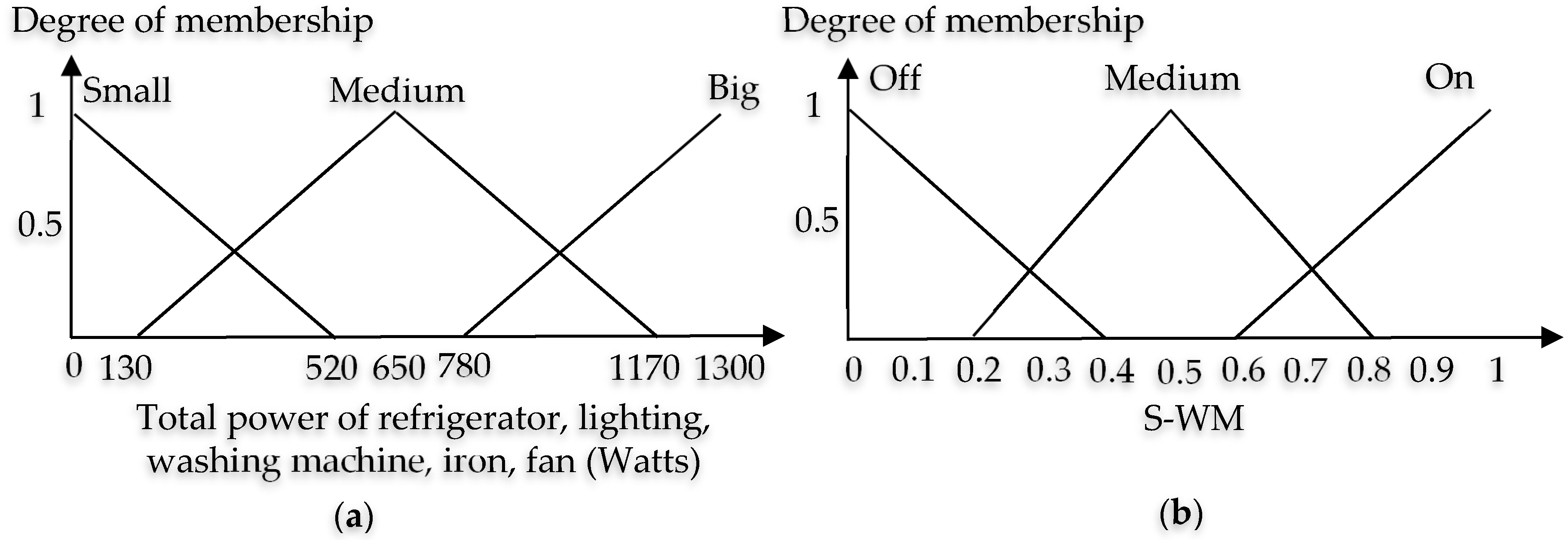
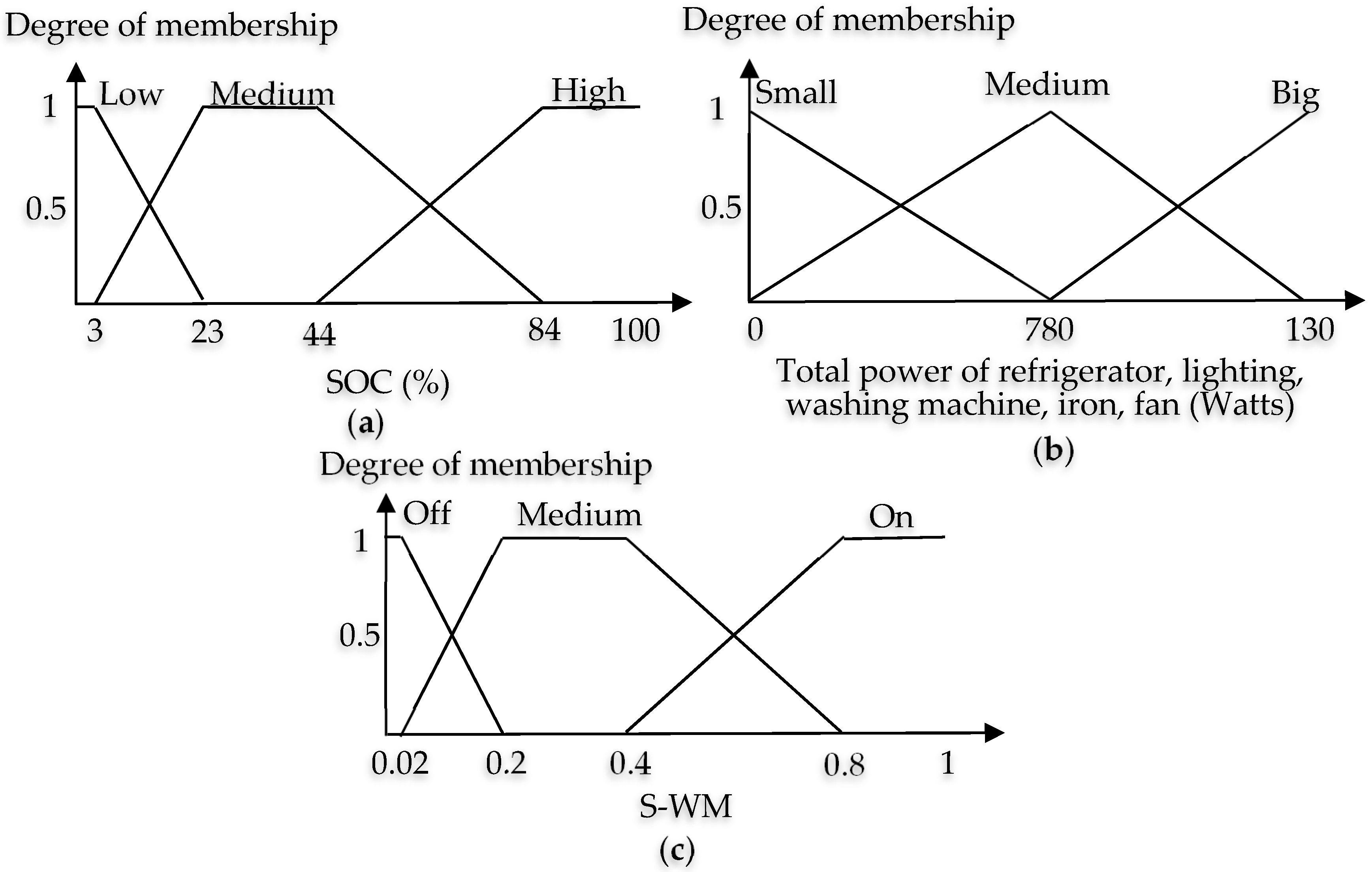
The membership function of the total power, including the refrigerator, lighting, washing machine, iron, and fan, is shown in
Figure 4a. This membership function is applied for the FLC-WM, the FLC-IR, the FLC-FAN, and the FLC-TV. The membership functions of S-WM, S-IR, S-FAN, S-TV are all the same, as shown in
Figure 4b.
2.2.2. Fuzzy Rules
The fuzzy rules for FLC-BAT are developed in such way that they comply with the objective, as given in
Table 2. The explanations of the rules are as follows:
IF PV power is Small AND SOC is Low THEN S-BAT is Off.
This means that when the energy from PV is small and the battery is empty (the capacity is low), then there is a high probability that the power switch will be off.
IF PV power is Small AND SOC is High THEN S-BAT is On.
This means that even though the energy from PV is small, if the battery is full (the capacity if high), then there is a high probability that the power switch will be on.
IF PV power is Big AND SOC is High THEN S-BAT is On.
This means that when the energy from PV is big and the battery is full (the capacity is high), then there is a high probability that the power switch will be on.
The fuzzy rules of FLC-WM are given in
Table 3. The rules for FLC-IR, FLC-FAN, and FLC-TV were developed in a similar way and are explained below:
IF total load power is Small AND SOC is Low THEN S-WM is Off.
This means that when the total load power is small and the battery is empty (the capacity is low), then there is a high probability that the power switch will be off.
IF total load power is Big AND SOC is Low THEN S-WM is Off.
This means that even though the battery is full, since total load power is big, it is better to switch off the load; thus, there is a low probability that the power switch will be on.
IF total load power is Small AND SOC is High THEN S-WM is On.
This means that when the battery is full and total load power is small, the load will be switched on.
2.3. Tuning of Fuzzy Membership Function Using Genetic Algorithm
As described previously, since tuning the fuzzy membership function is not a trivial task, several methods have been employed to tune the parameters of the FLC automatically [
22,
23,
24,
25,
26,
27,
28]. In this work, we adopted the GA-based tuning method proposed in Ref. [
24]. Since the FLC in Ref. [
24] is used for position control, some modifications needed to be developed. To the best of our knowledge, there has been little research on the FLC-based HEMS that has considered FLC tuning. Ref. [
22] proposed an online GA-based fuzzy tuning that is implemented in a Linux embedded system. Since the GA runs online, the approach could not be implemented on our microcontroller-based embedded system.
In our approach, the fuzzy membership function is tuned offline using the GA. The Matlab-Simulink is employed during tuning. The procedure of GA-based tuning is as follows:
Initialize the GA;
Model the proposed FLC with Load Simulink;
Encode the membership functions into the GA chromosomes;
Run the GA;
Decode the GA chromosomes;
Run the Simulink model of the proposed FLC;
Calculate the fitness function;
Repeat for N-generations.
As described in
Section 2.2, the proposed FLC can be divided into two categories: (a) the FLC of the PV-battery system, and (b) the FLCs of the loads. Since the FLCs of the loads have similar structures, there are six fuzzy membership functions to be tuned: the SOC of FLC-BAT, the PV power, the S-BAT, the SOC of FLC-WM, the total power of the refrigerator, lighting, washing machine, iron, and fan, and the S-WM. Each membership function is encoded into 7 bits—3 bits represent the offset field and 4 bits represent the companding factor [
24]. The offset field is used to change the shape of the membership function, while the companding factor is used to extend or compress the membership function. Readers are referred to Ref. [
24] for further detail.
The fitness function for evaluating the GA was developed in accordance with the HEMS objective—to minimize the electricity cost. The fitness function is calculated by running the Simulink model of the proposed FLC using the membership functions which are decoded from the GA chromosome. To calculate the fitness function, the model is run under two PV power conditions. In the first condition, the profiles of PV power are set to high values, while, the second condition uses low values. In each condition, the energy extracted from the grid is calculated. The fitness function is defined as the average value of the extracted grid power from both conditions.
2.4. Wireless Communication Configuration
The low-cost ESP-8266 WiFi module (Espressif Systems, Shanghai, China) was employed to perform wireless communication. In this work, we used the WeMos module [
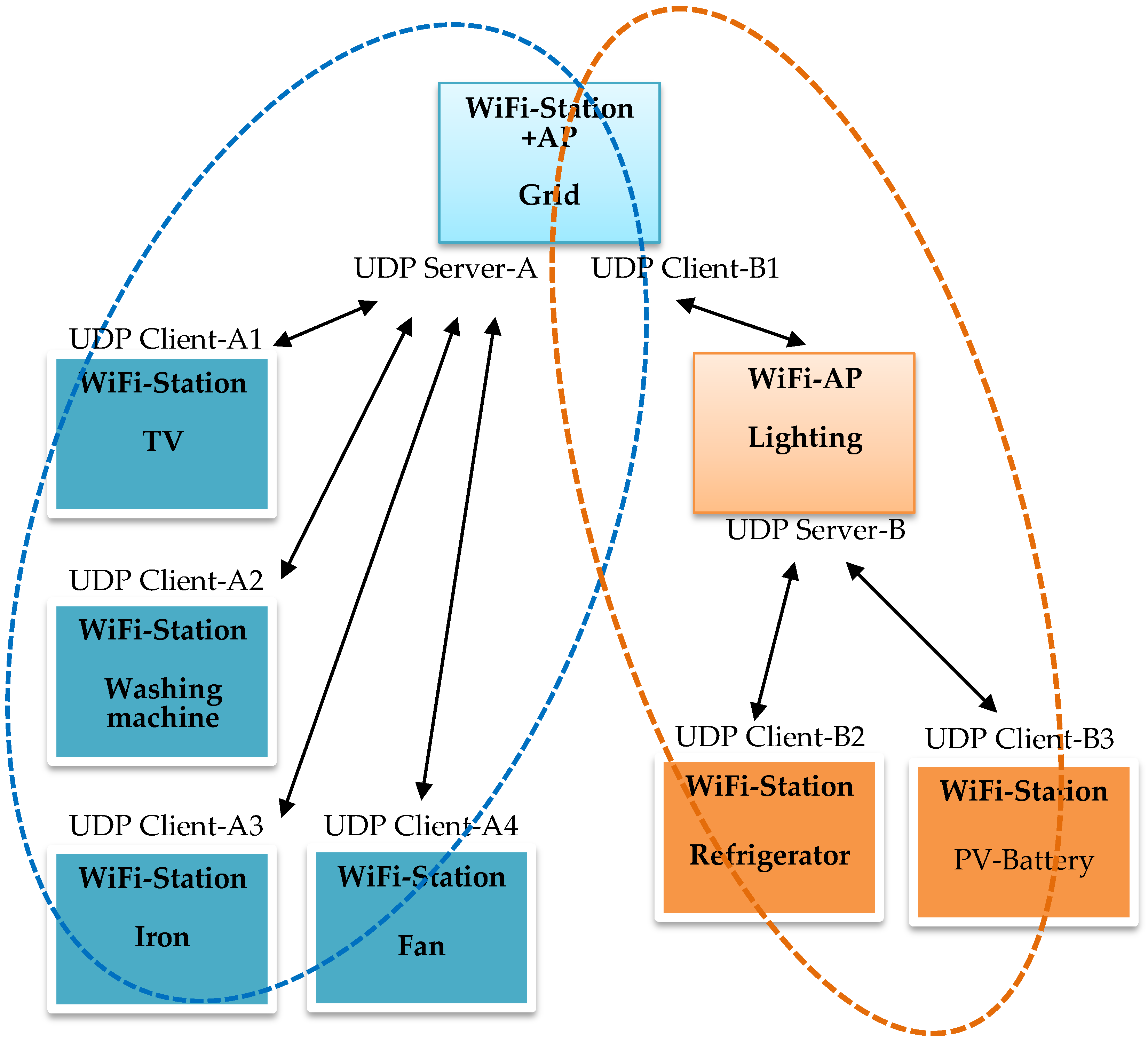
29] in which the WiFi unit is embedded in the Arduino board. This module provides a low-cost effective embedded system to implement the proposed FLC-based HEMS system. Since the ESP-8266 has a limited number of clients, we configured the wireless communication network as depicted in
Figure 5.
In WLAN-A, the WiFi AP (Access Point) is configured on the grid, while the WiFi stations are configured on the TV, the washing machine, the iron, and the fan. In WLAN-B, the WiFi AP is configured on the lighting, while the WiFi stations are configured on the grid, the refrigerator, and the PV-battery. It is noted that the WiFi module on the grid is configured as the AP and station. Through this arrangement, both WLAN-A and WLAN-B can exchange data via the WiFi module on the grid.
Both WLANs employ the User Datagram Protocol (UDP). In this configuration, the WiFi on the grid is assigned as both the UDP server and the UDP client, where it acts as the UDP server in the WLAN-A and the UDP client in the WLAN-B. In the WLAN-A, the WiFi modules on the TV, the washing machine, the iron and the fan act as the UDP clients. In the WLAN-B, the WiFi modules on the lighting act as the UDP server, while the WiFi modules on the refrigerator and the PV-Battery act as the UDP client.
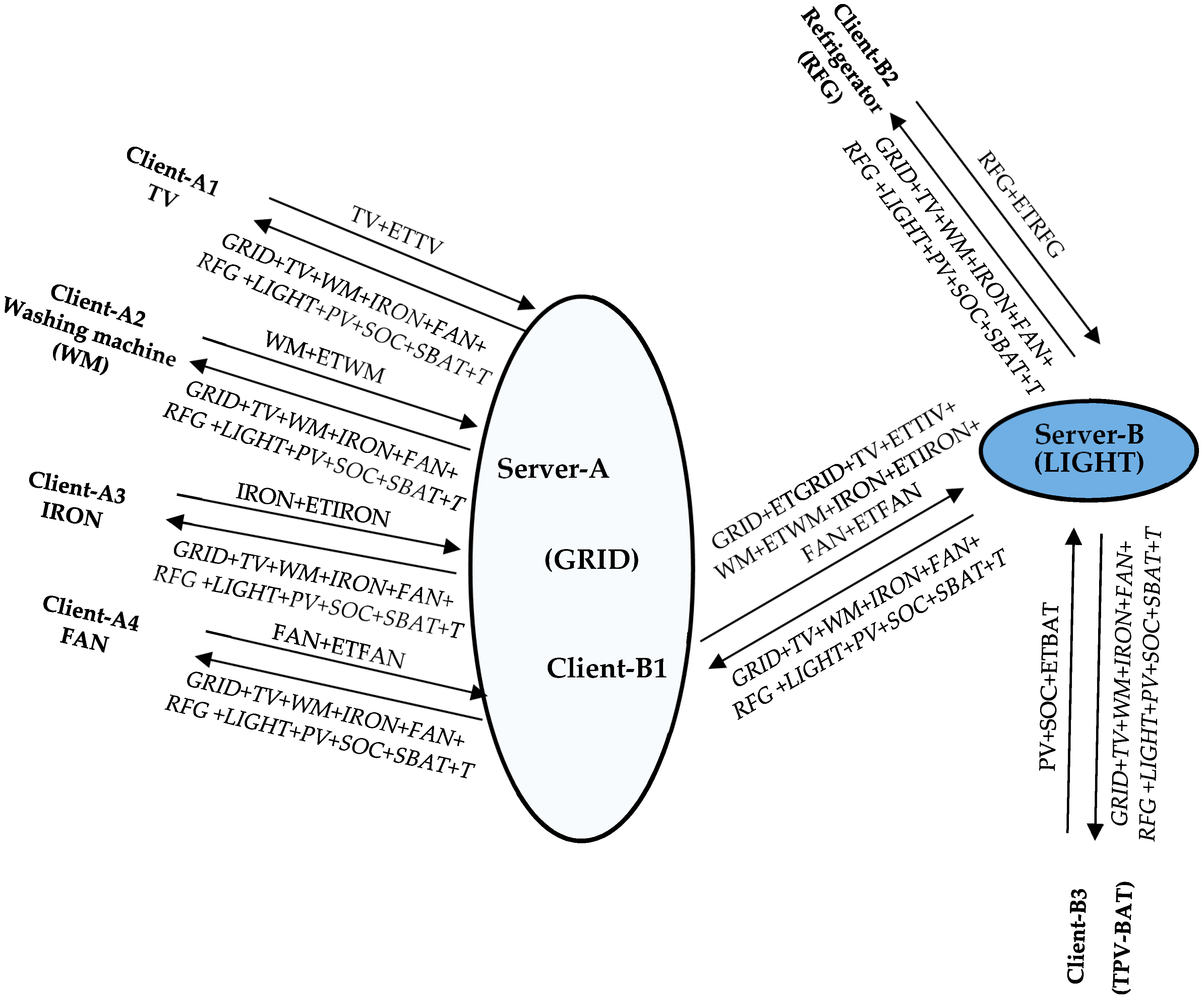
As discussed previously, each FLC requires data from all loads; thus, it is important to design the data communication protocol to satisfy this requirement using the proposed wireless communication infrastructure. The proposed data communication protocol is depicted in
Figure 6. As shown in the figure, each load sends its power consumption data to the server. For example, the washing machine (WM) sends “WM+ETWM” to server A (the grid). The “WM” is the power consumed by the washing machine. The “ETWM” is the execution time of the FLC module performed on the washing machine. The execution time data is used for measurement only.
Once the data is received by the server, the server will send the complete data as follows: “GRID + TV + WM + IRON + FAN + RFG + LIGHT + PV + SOC + SBAT + T”, where “GRID” is the power delivered from the grid; “TV”, “WM”, “IRON”, “FAN”, “RFG”, and “LIGHT” are the amounts of power consumed by the TV, the washing machine, the iron, the fan, the refrigerator, and the lighting respectively; “PV” is the power generated from the PV; “SOC” is the SOC of the battery; “SBAT” is the status of the power switch in the PV-Battery system (S-BAT). “T” is the time required for synchronization.
The figure shows that the data required by the FLC on each load is available after the load has sent the data to the server. Therefore, to maintain up-to-date data, the load should send the data to the server regularly. Since the HEMS algorithm is usually updated hourly or daily, our approach can feasibly be implemented. It is worth noting that the proposed communication architecture can be easily extended to cover the larger residential loads.
3. Experimental Results and Discussion
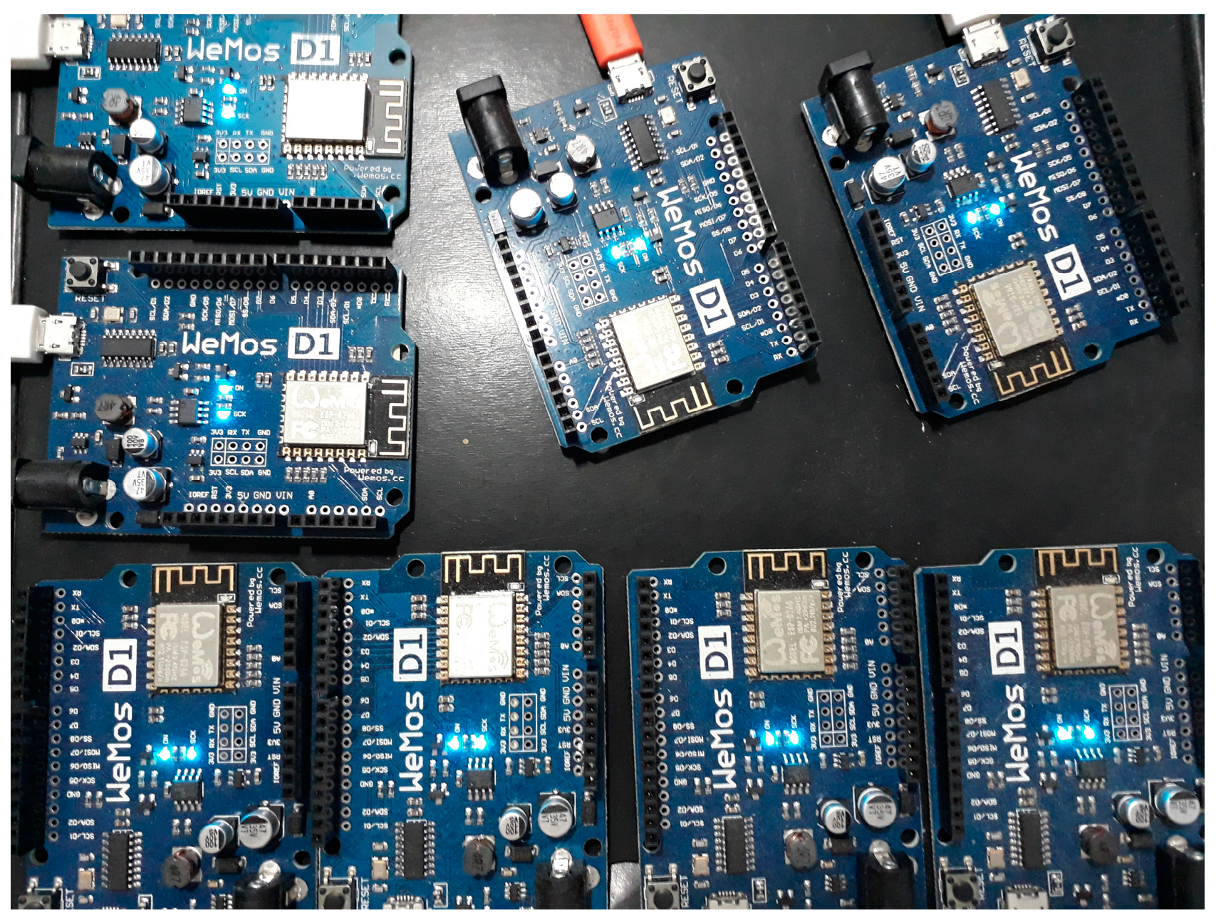
The proposed approach was validated using several experiments. The objective was to examine the feasibility of implementing the wireless communication and the FLC in the HEMS, in the terms of the execution time required to run FLC on the embedded platform, the data transmission time interval, and the effectiveness of FLC in reducing the electricity cost. In the experiments, the PV and load power data were stored in the memory of microcontroller. The hardware used in the experiments included eight WeMos modules, as illustrated in
Figure 7. The configuration of the WiFi on the modules is shown in
Figure 5.
The experiments showed that the amount of WeMos memory used by the FLC-BAT (the profile of PV power data is neglected) was 33,040 bytes from a maximum of 81,920 bytes (40.33%), while the FLC-WM (the load data is neglected) required a memory of 32,960 bytes from a maximum of 81,920 bytes (40.23%). It is clear that when the FLC is implemented on a central unit (centralized approach), it will consume about 80% of the WeMos memory. Furthermore, when each load has the different fuzzy rules and/or fuzzy membership functions, the FLC cannot be implemented on the WeMos module anymore.
3.1. Execution Time and Data Transmission Time Interval
As described in
Section 2.4, each WeMos module sends the power consumption and execution time data to the server. The data of all modules is collected by Server B, i.e., the WeMos module on the lighting. Therefore, the WeMos module on the lighting is connected to a personal computer to store all data sent by the modules. The measurement of the execution time and data transmission time interval are performed based on the collected data.
Due to the different processes performed on each WeMos module, it is divided into two categories:
Data communication only: The lighting (LIGHT), grid (GRID), and refrigerator (RFG) modules.
Data communication and FLC: The washing machine (WM), the iron (IRON), the TV (TV), the fan (FAN), and PV-Battery system (PV-BAT) modules.
The measurement results are given in
Table 4. The table shows that the execution time of the proposed embedded FLC system is very fast for this application. The largest execution time was achieved by the GRID, i.e., 26.98 ms. This is because the GRID performs the complex tasks in the data communication process as the server and the client simultaneously. The smallest execution time was achieved by the LIGHT, i.e., 0.14 ms. Since the LIGHT acts as a server only, the task is simple, i.e., it receives the data from the client and then replies to it. Therefore, the execution time is very fast. However, even though the RFG performs data communication only, its execution time is greater than that of the LIGHT, because it introduces a delay on the client side. It first sends the data to the server, and then it is delayed for a while (about 6 ms) to receive the data reply.
The table shows that the execution time of the FLC and the data communication is about 20 ms. Since the execution time of the data communication (client) is about 6 ms, the execution time of the FLC itself is about 14 ms.
The proposed FLC runs in the distributed scheme, where the data required by the FLC is received wirelessly. In this experiment, we examined the data transmission time to investigate the real-time processing of the embedded FLC. Under actual conditions, the proposed HEMS algorithm (i.e., to minimize the electricity cost by load shifting) will run on an hourly basis. The previous result shows that the proposed embedded FLC runs very fast, thus it can handle the hourly load scheduling problem. However, here, we investigated the fastest data communication time that can be handled by the proposed system in order to improve or extend the HEMS problem which runs on the basis of minutes or seconds.
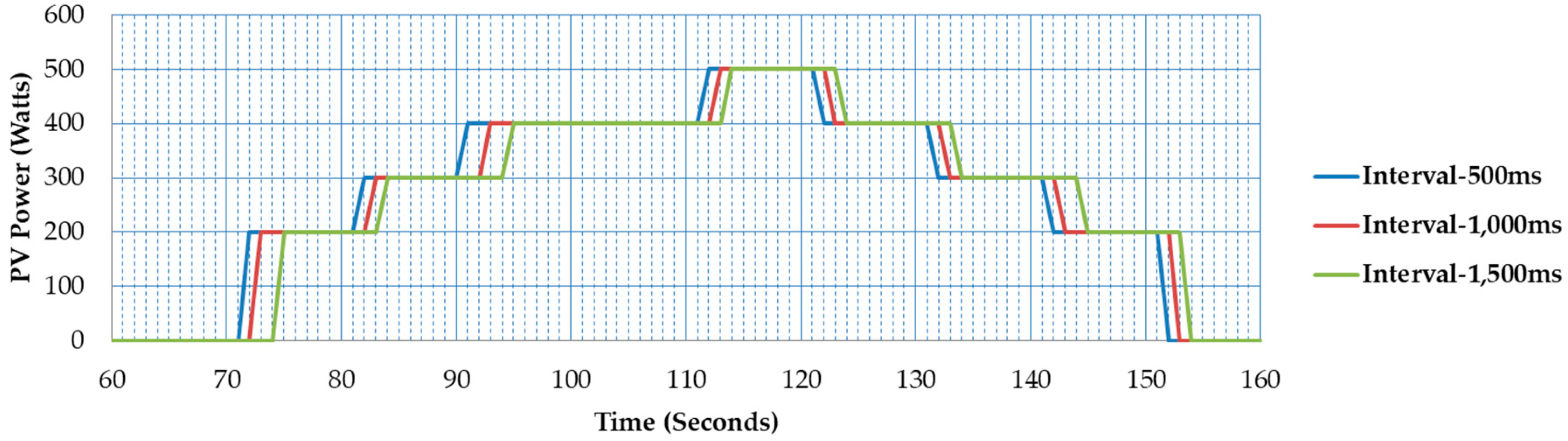
To measure the data transmission interval, we ran our system by simulating the hourly basis operation on a 10-s basis. This means that a one-hour long operation was simulated in 10 s. For example,
Figure 8 shows the profile of PV power generated by the WeMos module from 60 s to 160 s that represents the time from 6:00 a.m. to 4:00 p.m. (16:00 h). The effect of the data transmission interval is described below.
Figure 6 shows that the updated data required by the FLC in each WeMos module is obtained when the module sends the data to the server and the server replies with the whole set of data. Therefore, the WeMos module should send data continuously over a certain time interval. The selection of the time interval is important, since an insufficient time interval will lead to traffic in the WLAN, while an excessive time interval will delay the updated time. In the experiments, we examined three time intervals: 500 ms, 1000 ms, and 1500 ms. (t is noted from a few experiments that the time interval of 100 ms means some WiFi modules (WeMos) are unable to join the network. It is clear that the time interval affects the time basis of the HEMS algorithm in, in this case, on a 10-s or 5-s basis.
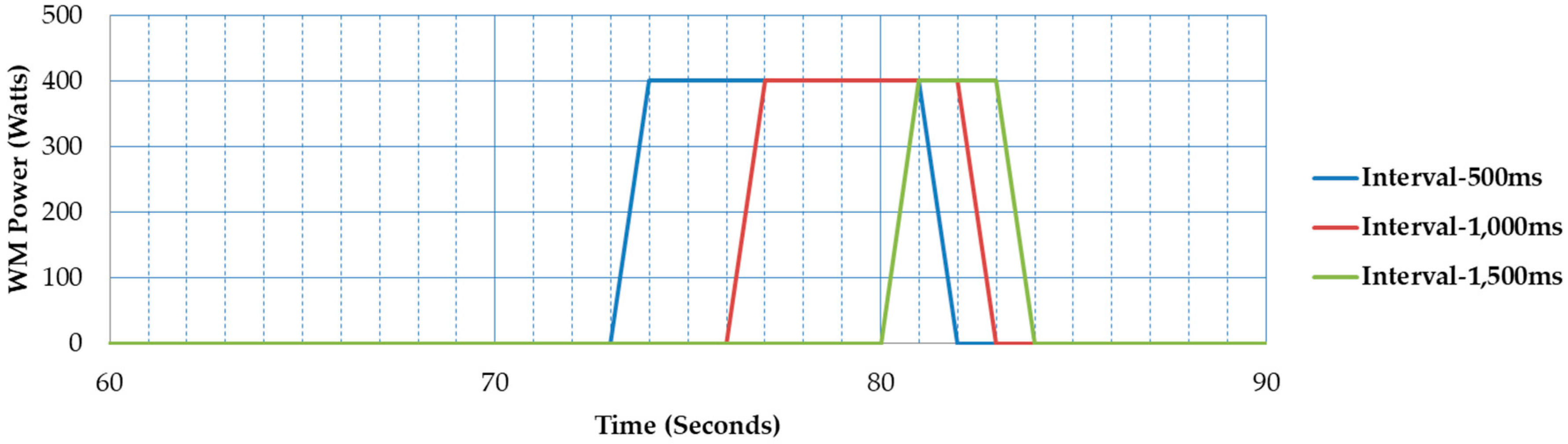
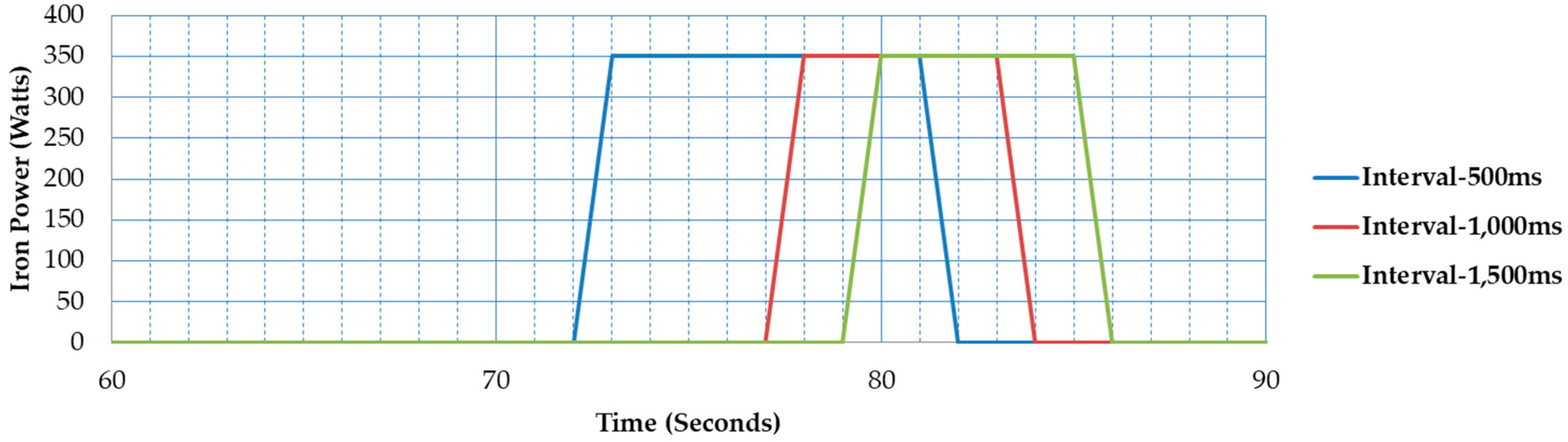
The profiles of the PV, washing machine, and iron power consumptions using a 10-s basis are depicted in
Figure 8,
Figure 9 and
Figure 10.
Figure 8 shows that the three data transmission intervals used introduced delays into the system so that the data received by the system was delayed several seconds from the original. For example, the green line (interval of 1500 ms) showed that the PV power of 200 Watt in the beginning was reached in 75 s; thus, it was delayed by 5 s from 70 s (recall that 70 s represents 7:00 a.m.). Fortunately, these delays did not exceed 10 s, thus the 10-s basis was sufficient. The different situations are shown in
Figure 9 and
Figure 10 for the time interval of 1500 ms. The green lines show that the delays were in excess of 10 s. Thus, the time interval of 1500 ms cannot be used when operating on a 10-s basis. The results suggest that our proposed system can be operated on a 10-s basis when the data transmission interval of each WiMos module is 500 ms. Therefore, the proposed embedded system can be feasibly implemented in HEMS algorithms that work on an hourly basis, such as the load scheduling problem.
3.2. FLC-Based HEMS Effectiveness
To examine the effectiveness of our proposed FLC algorithm, we tested it using four scenarios. The profiles of PV power are given in
Table 5. Each scenario used the same load data, which are given in
Table 6. The non-controlled loads (RFG and LIGHT) operated according to the specifications given in the table. For the controlled loads (WM, IRON, FAN, TV), the operation starting time was defined by the FLC, which is in the range of data given in the table and the operation duration follows the table. There were two cases in the operation starting time of the iron: in Case A, the starting time was at 05:00 h and in Case B, the starting time was at 12:00 h. The consumption power of the fan had three values, 40, 60, and 80 Watts, and was selected according to the FLC. In the experiments, the system ran on a 10-s basis, as described previously, i.e., hourly data was simulated in 10 s.
In the experiments, we compared two FLC systems: (a) A system in which the membership functions are defined manually, as described in
Section 2.2 (called FLC); and (b) a system in which the membership functions are tuned by the GA (called GAFLC). The tuned membership functions are depicted in
Figure 11 and
Figure 12. The GA parameters used to tune the membership functions were as follows:
To show the effectiveness of the proposed FLC in reducing the electricity cost, we compared three methods: (a) the No-FLC method, (b) the FLC method, and (c) the GAFLC method. In the No-FLC method, the controlled loads were assumed to operate as follows: the WM operates from 05:00 h to 06:00 h, the IRON operates from 14:00 h to 15:00 h, the FAN operates from 10:00 h to 18:00 h (60 Watt), and the TV operates from 17:00 h to 24:00 h. In this work, for simplicity, the electricity cost was determined by the price of electricity from the utility grid, i.e., 1 Watt hour was IDR 1.467. The prices of the PV-battery system were not considered. This assumption is reasonable, since we compared the methods using the same PV-battery system. The objective of the comparison was to examine the FLC method to solve the load scheduling problem.
The comparison results are given in
Table 7 and
Table 8. In the tables, FLC-A and FLC-B are the results of the FLC method when the iron was operated in Case A and Case B, respectively, while GAFLC A and GAFLC B are the results of the GAFLC-method when the iron was operated in Case A and Case B respectively. To provide easy understanding, the grid power profiles in Scenario 1 to Scenario4 are depicted in
Figure 13,
Figure 14,
Figure 15 and
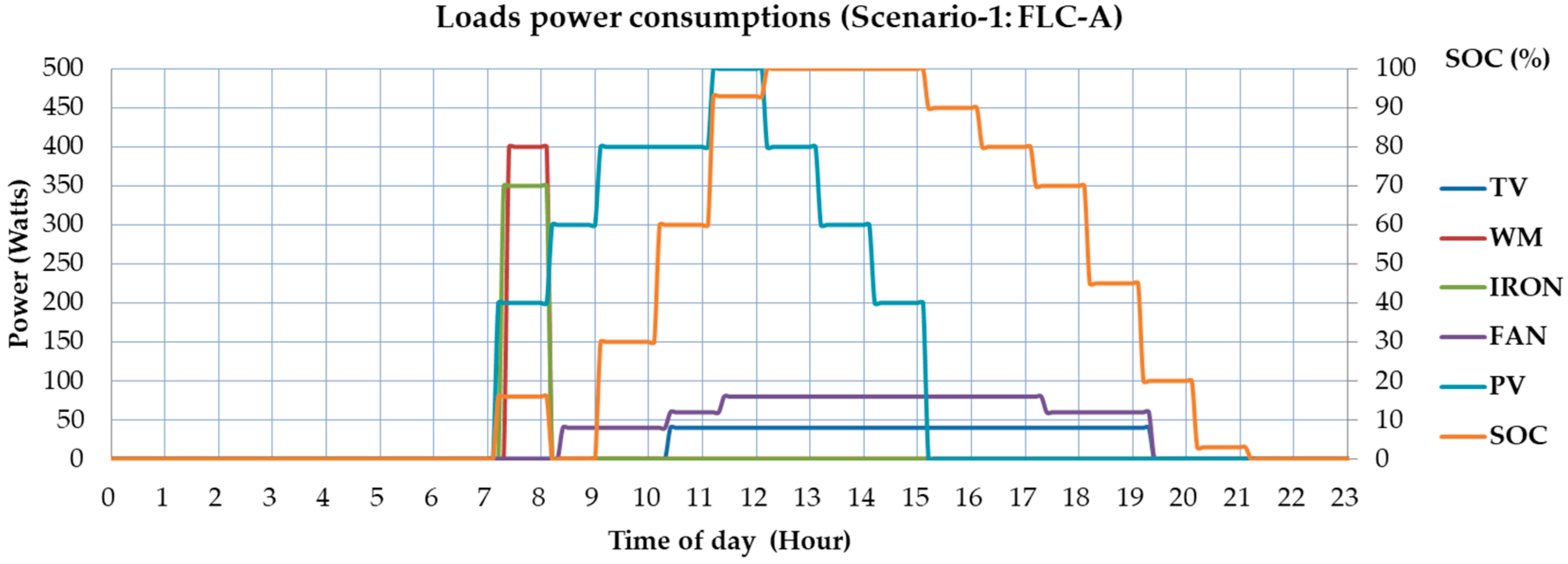
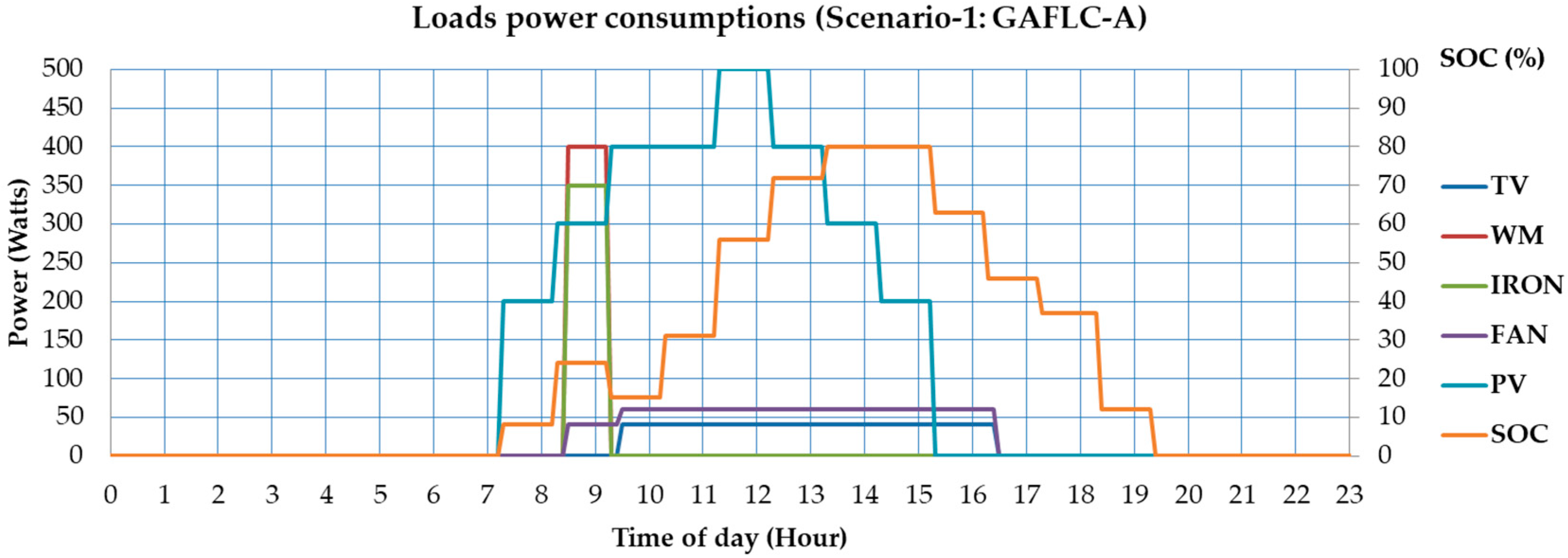
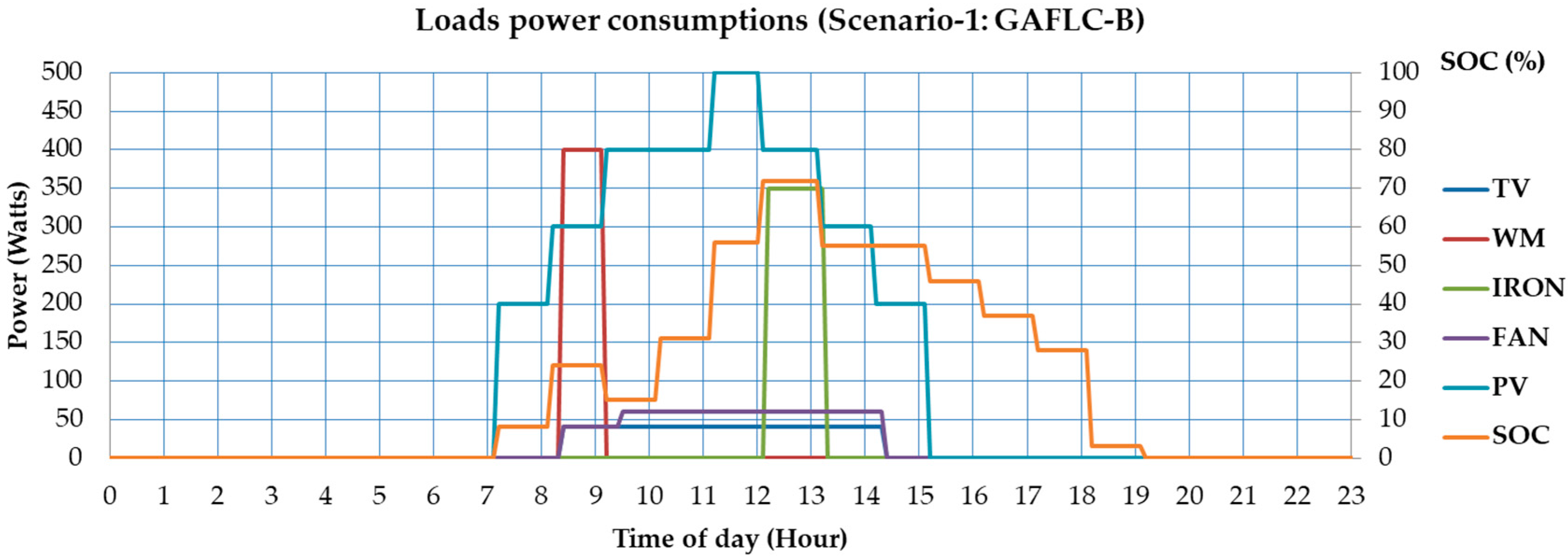
Figure 16, while the load power consumptions of the four methods (FLC-A, FLC-B, GAFLC-A, GAFLC-B) in Scenario 1 are depicted in
Figure 17,
Figure 18,
Figure 19 and
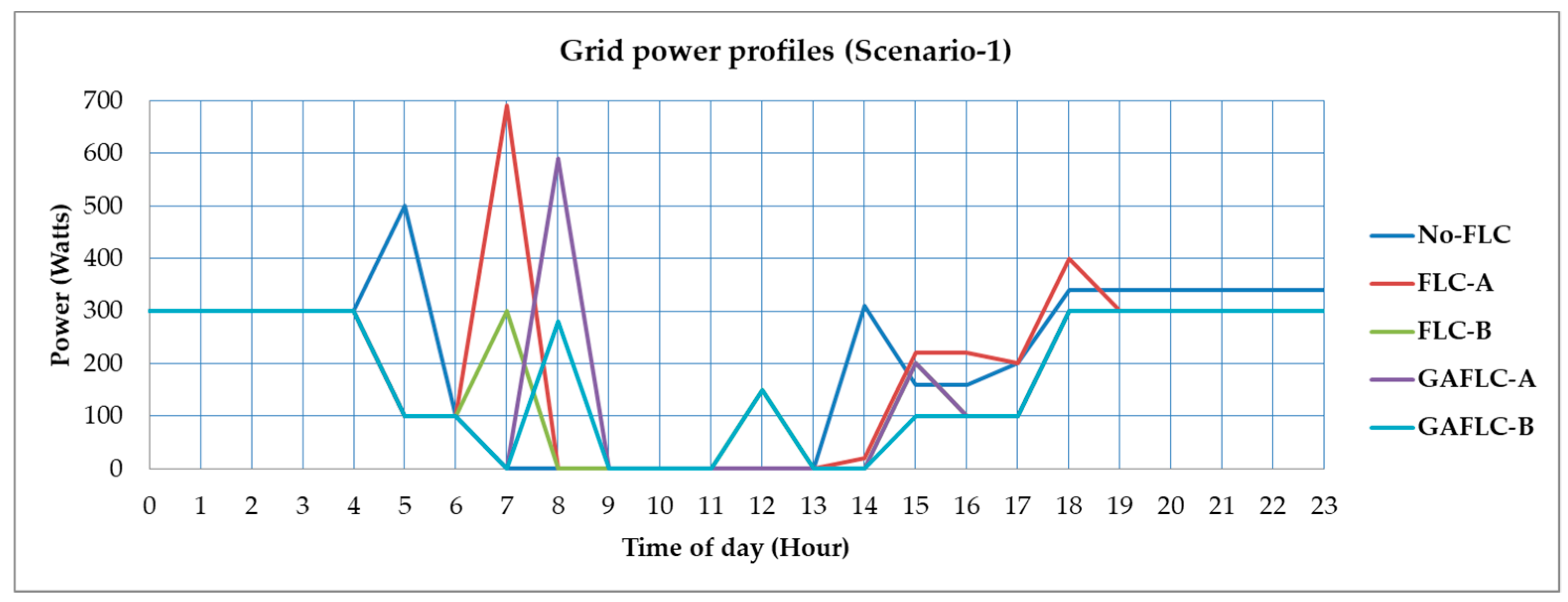
Figure 20. From the results, we obtained several findings, as follows:
The electricity costs of both the FLC method and the GAFLC method were lower than the No-FLC method. The average cost reduction of the four scenarios was from 3.865% to 12.493%. By examining
Figure 13, it is interesting to analyse when the peak power levels occurred (i.e., when the WM and/or the IRON was switched on). In the No-FLC, they occurred at 05:00 h (the WM was switched on) and 14:00 h (the IRON was switched on). The total power drawn from the grid was 500 + 300 = 800 Watts. In FLC-A, this occurred at 7:00 h, when the total power drawn from the grid was 690 Watt. In FLC-B, this occurred at 7:00 h and 12:00 h, when the total power drawn from the grid was 300 + 150 = 450 Watt. In GAFLC-A, this occurred at 8:00 h, when the total power drawn from the grid was 590 Watt. In the GAFLC-B, this occurred at 8:00 h and 12:00 h, when the total power drawn from the grid was 280 + 150 = 430 Watts. Similar conditions also occurred in
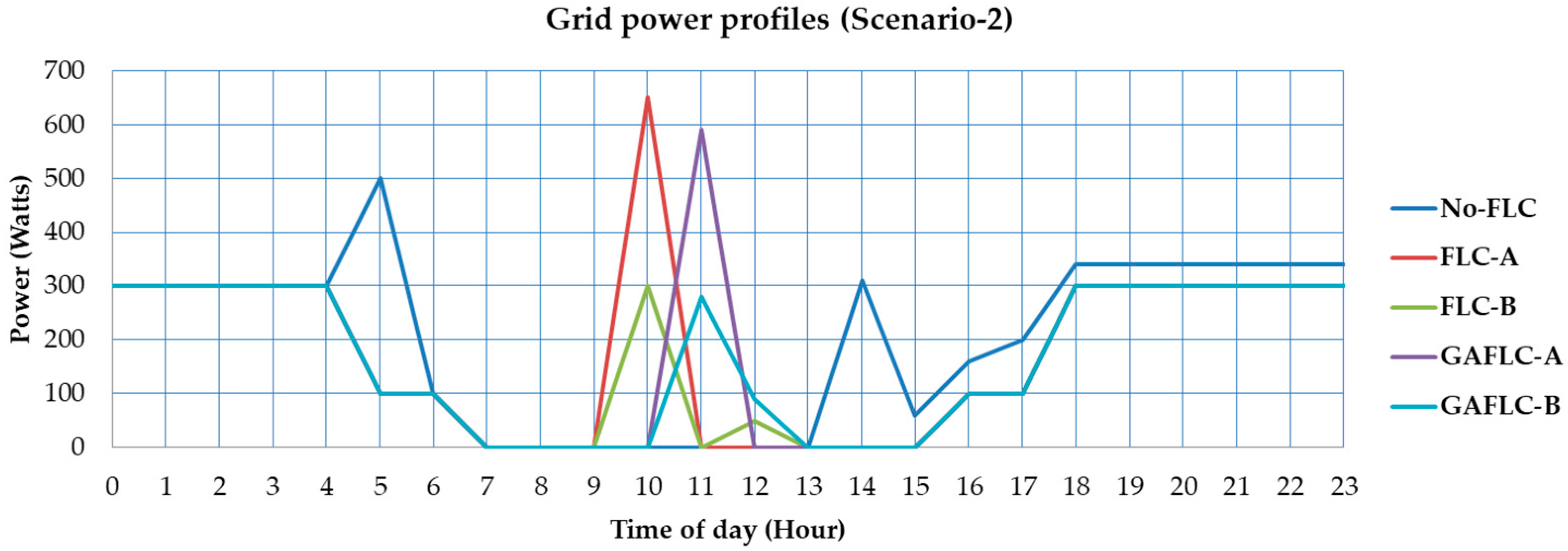
Figure 14,
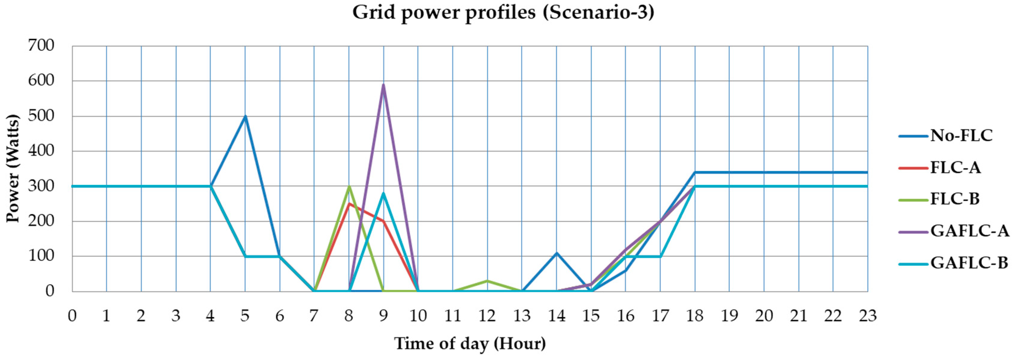
Figure 15 and
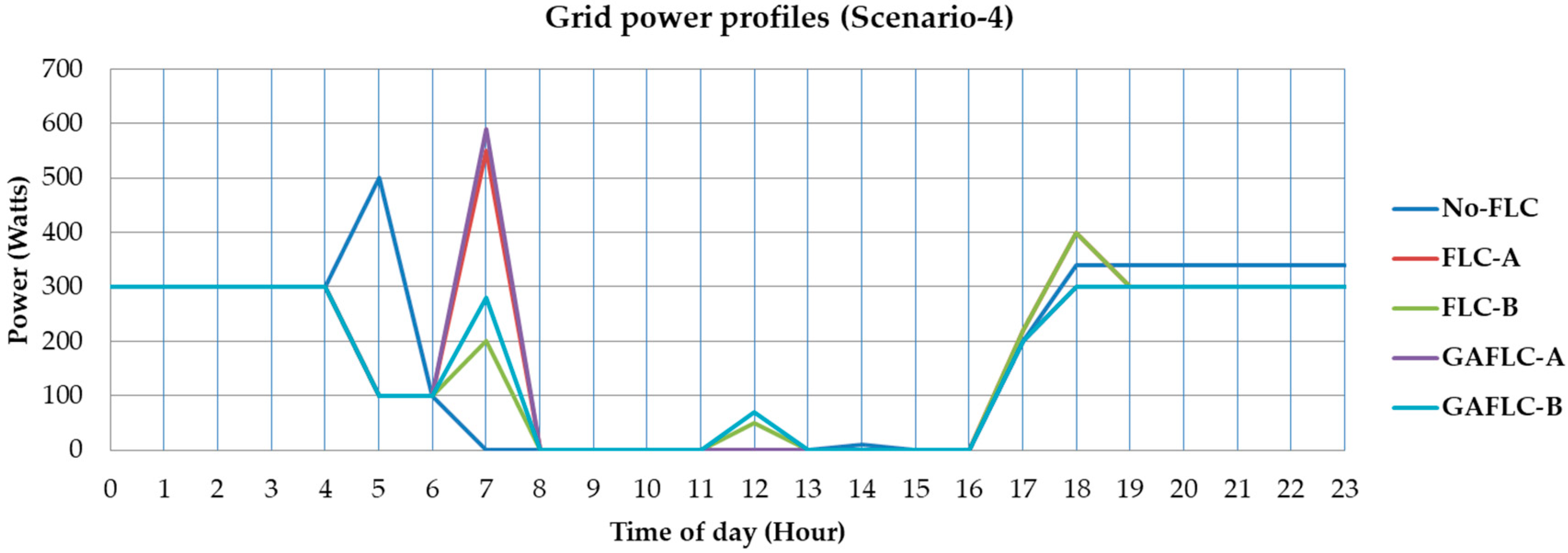
Figure 16. Since the peak power levels of the FLC and the GAFLC methods were lower than that of the No-FLC, it is clear that the FLC and GAFLC methods reduce the electricity cost.
It is noted here that in Scenario 4, the electricity cost of FLC-A was slightly higher than that of No-FLC. However, the GAFLC-A in Scenario-4 was able to reduce the electricity cost, even though only slightly. This strange result may have been caused by improper membership functions which were determined manually).
In both the FLC and GAFLC methods, the electricity cost of Case B was lower than that of Case A. Thus, by shifting the operation starting time of the iron to the afternoon, the excessive power from PV was consumed by the iron, thereby reducing the electricity usage from the grid. This is shown by
Figure 13 and
Figure 19, where the GAFLC-A operates the washing machine and the iron at 08:00 h and obtains 590 Watt of power from the grid, while
Figure 13 and
Figure 20 show that the GAFLC-B operates the washing machine at 08:00 h and the iron at 12:00 h. Thus, it obtains 280 + 150 = 430 Watts of power from the grid. Similar situations occurred in FLC-A and FLC-B. The average cost reduction increased from 3.875% (Case A) to 10.933% (Case B) in the FLC-method and from 6.189% (Case A) to 12.493% (Case B) in the GAFLC method.
In both Cases A and B, the average cost reduction of the GAFLC method was lower than that of the FLC method. In Case A, the average cost reduction increased from 3.875% (FLC method) to 6.180% (GAFLC method), while in Case B, the average cost reduction increased from 10.933% (FLC method) to 12.493% (GAFLC method). This shows that the automated tuning of the membership functions using the GA effectively improved the performance of FLC, i.e., increased the cost reduction.
Table 8 shows that the cost reductions in Scenarios 1 and 2 were higher than those in Scenarios 3 and 4. The results were analyzed by examining the PV profiles in
Table 5 and the operation starting times of the IRON in the No-FLC method, i.e. from 14:00 h to 15:00 h. Since the grid power profiles of all methods were almost the same from 16:00 h to 24:00 h (see
Figure 13,
Figure 14,
Figure 15 and
Figure 16), to analyze the cost reduction, we considered the time beyond that range, especially at 14:00 h when the IRON was switched on in the No-FLC method. In Scenarios 1 and 2, the level of PV power was relatively low during this time; thus, the 300 Watts of power should be drawn from the grid (see
Figure 13 and
Figure 14). However, in Scenarios 3 and 4, the PV power was relative high during this time; thus, only 100 Watts of power should be drawn from the grid in Scenario 3 (see
Figure 15), and no power should be drawn from the grid in Scenario 4 (see
Figure 16). Thus, the cost reductions in Scenarios 1 and 2 are higher than those in Scenarios 3 and 4.


