Abstract
This paper presents the design and construction of a robotic arm that plays chess against a human opponent, based on an artificial vision system. The mechanical design was an adaptation of the robotic arm proposed by the rapid prototyping laboratory FabLab RUC (Fabrication Laboratory of the University of Roskilde). Using the software Solidworks, a gripper with 4 joints was designed. An artificial vision system was developed for detecting the corners of the squares on a chessboard and performing image segmentation. Then, an image recognition model was trained using convolutional neural networks to detect the movements of pieces on the board. An image-based visual servoing system was designed using the Kanade–Lucas–Tomasi method, in order to locate the manipulator. Additionally, an Arduino development board was programmed to control and receive information from the robotic arm using Gcode commands. Results show that with the Stockfish chess game engine, the system is able to make game decisions and manipulate the pieces on the board. In this way, it was possible to implement a didactic robotic arm as a relevant application in data processing and decision-making for programmable automatons.
1. Introduction
The first machine to play chess was built in 1769 by Wolfgang von Kempelen and was known as “The Turk” [1]. Apparently, the machine could play chess against a human opponent, but it was actually operated by a chess master.
For many years, researchers in the area of artificial intelligence have been working on algorithms to play chess autonomously. Alan Turing and David Champernowne were the first to develop a program capable of playing a full chess game [2], known as “Turing’s paper machine” [3,4]. Because at the time there were no computers capable of executing the instructions, it was Turing himself who performed the processing tasks using paper and pencil. It was not until 1996 that a fully functional computer program, IBM’s Deep Blue, was able to defeat the world champion Gary Kasparov [5].
Since then, many chess engines have been developed, and simultaneously it has become easier to develop mechanical robots [6,7]. The chess game is an excellent application that works as a test bed for the implementation of autonomous robotic systems, as it requires solutions for perception, manipulation, and human–robot interactions for a well-structured problem [8,9,10,11,12].
Several alternatives have been used for the perception of game state in different implementations of autonomous chess systems. In [13,14], the authors focused on differentiating specific chess pieces, but the high levels of precision required by reliable autonomous systems were not achieved. Most practical implementations address this problem by detecting the movements of the pieces and tracking them from their initial position, assuming that the initial configuration of the board is correct.
In [15,16], the researchers used on-board magnetic sensors to detect the movement of the pieces, and a fixed position for the board relative to the robot in order to ease the manipulation [17,18,19]. Other works used 2D and depth cameras to follow the development of the game [20,21,22,23,24], while in the investigation carried out in [25], depth cameras were used to detect the occupancy of the board squares and compare the current state with the previous states.
In this work, a single 2D fisheye camera mounted on the arm grip was used for all perception tasks. Most of the implementations reported in the literature and chess game tracking systems with 2D cameras use variations of color-based comparisons [26], image subtraction methods to detect changes [27], and border detectors in order to detect the occupancy of the board squares [28].
Color-based and image subtraction methods require chess sets for a substantial color contrast between the board and the pieces; thus, these methods are not robust to lighting changes. Edge-based methods work well with chess sets with low color contrast, but are prone to misinterpret shadows on empty squares.
The main novelty of this work is the use of a hybrid Siamese network that is responsible for the detection of position changes of the pieces using a comparison layer, and the color classification of pieces using a classification layer. Class classification was used to verify the board initial configuration and was useful in speeding up the data tagging during the database creation [29,30].
The Siamese network approach for the detection of changes provided good results in extreme cases of movement of pieces with very little background color contrast (such as for white pieces on a white background). In addition, the method is very robust for changes in lighting.
The implementation uses an image-based visual servoing algorithm (IBVS) [31] based on the Kanade–Lucas–Tomasi feature tracker (KLT) to position the grip [32]. Therefore, the system does not depend on a fixed position for the board relative to the robot to manipulate the pieces.
This work focuses on vision algorithms and their integration with the mechanical system. The main goal was the design of a didactic robot for research purposes.
2. Materials and Methods
The structure of the system consists of a computer connected to an Arduino board, which is responsible for controlling the motors of the robotic arm using two TB6560 stepper drivers. The system incorporates a 170-degree fisheye camera [33] mounted on the arm grip and connected to the computer via USB (see Figure 1).
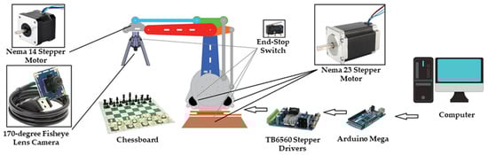
Figure 1.
General block diagram of the system.
2.1. Robotic Arm Design
The design used for the robot structure was made by the rapid prototyping laboratory FabLab RUC of the University of Roskilde, Denmark. It is an open design that includes CNC (Computer Numerical Control) diagrams for laser cutting and some software elements that were not used in this work.
The original design was conceived to be cut in 12 mm plywood and to use Nema 42 stepper motors. However, the cost of these motors together with their drivers exceeded the project budget. For this reason, modifications were made to the original design and all parts were resized by a factor of two-thirds (see Figure 2a). This modification made it possible to replace the original Nema 42 motors with smaller Nema 23 motors (see Figure 2b). Additionally, the thickness of the plywood was reduced from 12 mm to 9 mm.
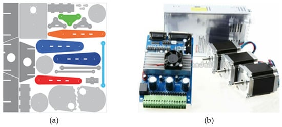
Figure 2.
(a) Robotic arm parts for laser cutting; (b) Nema 23 stepper motors, driver, and power supply.
To provide an initial reference position for joints, end-stop switches were used for each stepper motor (three on the rotation axes and one for the gripper).
Gripper Design
A four-finger gripper was designed using Solidworks software and subsequently printed using an Ultimaker 3D printer (See Figure 3). This was different from the design proposed by FabLab RUC. A Nema 14 stepper motor coupled to a worm was used with a linear gear to open and close the gripper fingers [34]. The design allowed the camera to be coupled in the center of the gripper.
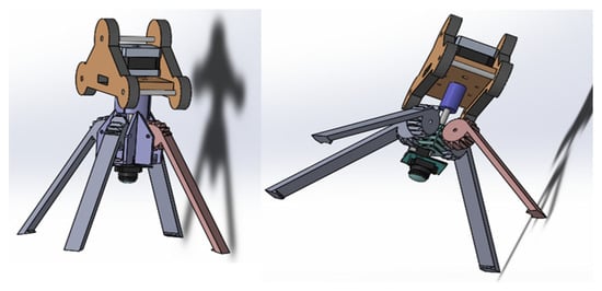
Figure 3.
Design made in Solidworks for the gripper.
2.2. Control Stage with Arduino
An Arduino Mega 2560 was used, functioning as an interface between the computer and the stepper driver. The Arduino is also connected to the end-stop switches, which are triggered in the starting position of the motors. The drivers are controlled through the digital pins.
2.2.1. Stepper Drivers
The TB6560 driver supplies power to Nema 23 motors installed in the three rotational axes. The interface with the TB6560 driver was performed using the parallel port in manual operation mode (see Figure 4a). For each motor, the activation, direction, and step pins were used. The limit pins for the three axes were not used, since this task was performed by the Arduino with the end-stop switches.
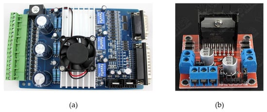
Figure 4.
(a) TB6560 stepper motor driver. (b) L298N motor driver module.
The driver module was set to one-half micro steps. Initially tests were performed with smaller micro steps, but the torque needed to move the arm was not achieved. Additionally, an L298N module was used [35,36] to control the speed of the Nema 14 motor of the gripper (see Figure 4b).
2.2.2. G-Code Commands
In order to facilitate the control of the robotic arm, a set of G-code commands was implemented [37], which was received by the Arduino serial port.
G1: This command generates a linear path from the current position to the desired coordinate for the motors. If the arm is in motion during the command reception, the final coordinate is rewritten and the direction of movement changes. If the arm position is unknown (before the end-stop switches are triggered), no movement is made, since the joints can collide. During the movement, the Arduino sends the current arm position to the computer.
G28: All motors move in the direction of the end-stops switches, with the positions set to zero. Although in most CNC machines the axes move one by one, in this case axes A and B move at the same time, because of the mechanical constraints of the workspace of robot (see Figure 5).
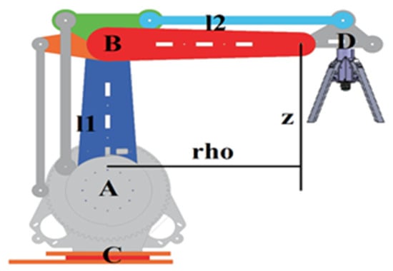
Figure 5.
Axes of the robotic arm.
When the end-stops switches are triggered, the Arduino sends the initial position through the serial port. This was useful to establish the mechanical constraints of the robot.
M18: Disable all stepper motors. It is possible to move the robot manually.
M17: Enable all stepper motors, with their position remaining unknown.
M114: The Arduino sends the current position of the motors through the serial port. This code is useful for debugging purposes.
2.3. Computer Software
A computer application handles the high-level processing tasks. The software was written in Python 3.6, because it has libraries suitable for image processing and the design of neural network models.
2.3.1. Image Capture and Preprocessing
A fisheye camera lens with an angle of view of 170 degrees was used in order to cover the whole chessboard. This camera has a good angle of view, but the lens distorts the captured image; thus, it was necessary to implement an image correction model. Therefore, a calibration process was done with an asymmetric chessboard and several image samples, using the tools incorporated in the OpenCV (Open Source Computer Vision) library [38,39].
2.3.2. Chessboard Corner Detection and Image Segmentation
A corner detection algorithm is required for several reasons, including searching the board during game initiation, image segmentation of the pieces for the recognition model, and definition of the tracking point in the visual servoing system during the piece-grabbing process.
The first stage of the corner detection algorithm consists of finding straight lines in the image. For this, the Canny edge detector [40,41,42] and the Hough transform [43,44,45,46] were used, which are available in the OpenCV library.
For each detected line, there is an associate pair (r, θ), where r is the distance from the origin of the image (upper left corner) to the closest point on the line, and θ is the angle between the x axis and the line connecting the origin to that closest point.
For the second stage of the process, kernel density estimation (KDE) [47] was used to find the two main groups of angles θ with a difference of 90 degrees, which correspond to the groups of vertical and horizontal lines. As long as there are not many parallel lines in the image, the angles of the chessboard lines correspond to the two highest peaks in the KDE (see Figure 6). The lines with angles distant to the board’s line angles were discarded.
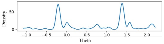
Figure 6.
Kernel density estimation (KDE) of the line angles.
The next step is to find the board lines. The KDE of distances r for the groups of vertical and horizontal lines was calculated. From this, nine peaks were found for each group.
In Figure 7, there is a smaller peak corresponding to the board edge line (red circle at the right). When checking the average distance between the peaks, the board edge lines are also filtered.
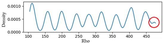
Figure 7.
KDE of rho distances for vertical or horizontal group of lines. The peak in the red circle corresponds to one of the board’s edge lines.
The Hough transform finds several redundant lines in the image for every line on the chessboard. Each peak on the r KDE is used as an estimate of the local averages for every subgroup of redundant lines in order to estimate the r values of the board lines. The θ angles of the board lines are independently computed with the average θ of the redundant subgroup of lines, since the real lines in the image are not perfectly parallel with each other. The chessboard corners are found by intersecting the predicted vertical and horizontal lines.
2.3.3. Change Detection and Class Classification
After the chessboard corner detection, the image is segmented and used for the movement detection and classification of the pieces and background colors. The system follows the pieces during the game, using the change detection to track their movements from their initial positions.
Initially, different models were tested for the color classification (namely, logistic regression [48], fully connected neural networks [49], and convolutional neural networks [50]). The best results were obtained with convolutional neural networks. The classes were classified as: white background, green background, white piece on a white background, white piece on green background, black piece on white background, and black piece on green background.
Later, a Siamese network [51,52,53,54] that compares the image of the current move with that of the previous move was designed in order to detect movements. The feature vector of the convolution stage was used for color recognition and for movement detection using additional network layers, but the vector from the previous movement image was used only for the comparison layer (see Figure 8).
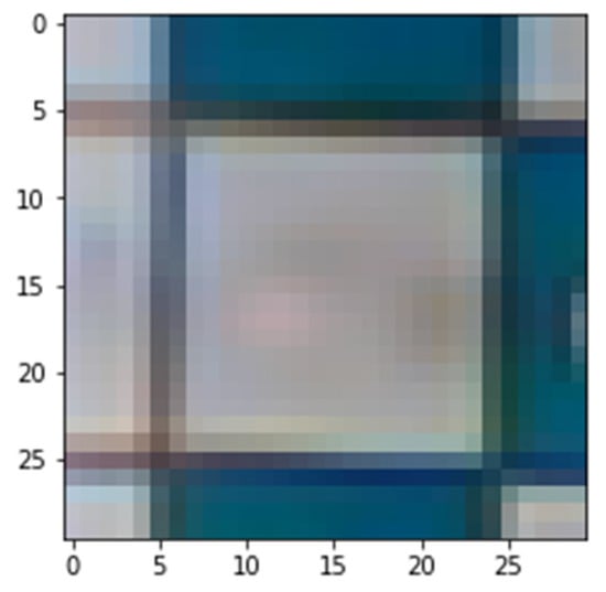
Figure 8.
Example of white piece on a white background.
The change detection was solved using the Siamese network, because in the case of white pieces on a white background, the color contrast is very subtle (see Figure 8). The use of methods such as color comparison and image subtraction is not suitable for these cases. Also, the use of class classification alone is not robust enough to compare the classification outputs to detect changes.
The model was designed using Keras. It has six outputs for the class classification, and one for the change detection (see Figure 9).
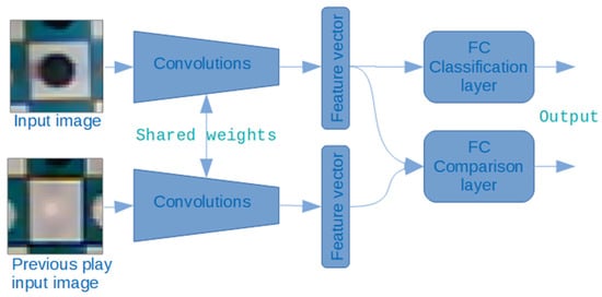
Figure 9.
Structure of the Siamese network (FC: Fully Connected).
Database collection: The software includes the option of making predictions using the current class classification model (to speed up the labelling process), a panel to label the data, and a save button to export a npz file with the image, board corners, and color labels. In this way, a database of 5 tagged images (320 tagged squares) was created.
For each image, the lighting conditions were purposely changed, the robot camera position was moved a few centimeters, and the pieces were slightly misplaced; this was done to obtain more realistic data.
Training: To perform the training, the images, corners, and labels from the npz files were imported. The images were trimmed using the corners as reference, with a padding equaling 25% of the square size; thus, the information for the surrounding squares facilitated the background color recognition. The images were scaled to a size of 30 x 30 pixels with three color channels.
The data were randomly separated into training and test data with a ratio of 8:2. To take better advantage of the data, the images were rotated and flipped. This process generated 8 images for each image in the original database.
2.3.4. Move Validation
The software uses the Stockfish chess engine for game decision-making and movement validation. The color prediction was used to verify the initial position of the board, while the change detector was used to track each movement of a piece from its initial position.
For the change detection, the comparison layer outputs a value between 0 and 1. Although it is not a probability function, it was used as a likability metric to predict the changes. Values close to zero represent little change, while values close to one represent a significant change. The use of this metric overcomes confusion when more than 2 squares appear to have changed, since the metric can present small changes for other reasons; for example, if the lighting varies or an adjacent piece casts a long shadow on the square.
Each movement involves a change in two squares (the castling and En passant are exceptions that are not handled properly). The likability of a movement is modeled with the product of the change metrics of the two squares involved. The prediction of the opponent movement is then the valid move with the highest likability for the squares with change metrics greater than 0.3.
2.3.5. Visual Servoing
From the robot resting position, the camera is able to see the whole board. To grab a chess piece, the target point is expressed using the corners and center of the square where the piece is situated (see Figure 10). However, during the movement, when the arm approaches the piece, the camera loses sight of the board corners and cannot be used to track the position of piece. For this reason, the Kanade–Lucas–Tomasi algorithm was used to track the piece during image-based visual servoing (IBVS). The depth information is obtained from the known kinematics of the robot [55,56].
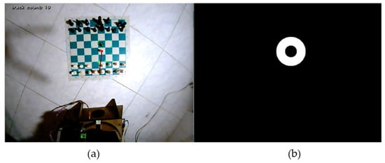
Figure 10.
(a) Tracking the point of interest (red) using reference points (green). (b) The mask used to find reference points.
Tracking a single point is not reliable. In addition, all the points in the image are not suitable for tracking; thus, a mask was implemented to find reference points around the target point (see Figure 10b). The reference points are paired, and for each pair, a prediction of the position of the target point is done for each frame. Two points are sufficient for each prediction, since the camera remains parallel to the plane of the board during movement; thus, the projective transformation of the image is neglectable.
2.3.6. Robot Calibration and Kinematics
To perform the calibration of the robot, a mapping is made between the stepper motor positions and the angles of the segments via linear regression (see Figure 11b). The angles were measured with the gyroscope from a cell phone. With the motors disabled, the robot moves manually to the position to be measured; thus, it is possible to use the G28 code to obtain the motor positions corresponding to the segment angles. Note that the angle of segment B is independent of motor A (see Figure 11a).
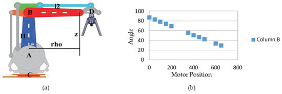
Figure 11.
(a) Segments, angles, and coordinates of the arm. (b) Angle vs. motor position for the segment.
The formulas for the end effector rho and z positions from which we start are:
During the piece-grabbing movement, the position of the robot is solved so it can hover over a point P, which is given by the visual servoing algorithm (see Figure 12). With each frame, the final position is recomputed and rectified.
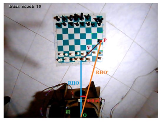
Figure 12.
Position unknown for the guide point.
Variables rho’ and ΔC (see Figure 12) are required to solve the position of the robot. Here, rho is obtained from the known kinematics of the robot. The vector V is converted from pixels to centimeters. The ratio of conversion depends on the camera height and was calculated using a linear regression, for which distance measurements were made at different camera heights (see Figure 13). Using rho and V, is easy to find rho’ and ΔC.
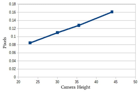
Figure 13.
Relationship between centimeters and pixels with the camera height.
To solve the inverse kinematics, a penalty method was used with the square error of the position as a function J to minimize. This function finds the angles A and B for the desired rho’ and z coordinates. Here, rho’ is calculated with the visual servoing system, and z is fixed depending on the task or piece to be grasped.
Since J is minimized for only two variables, a simple two-step exhaustive search is done, first for several scattered values of A and B, then for all the values close to the first solution. Here, mask is a Boolean matrix that penalizes the regions corresponding to the mechanical restrictions of the arm. The J function has a single local minimum because the arm joints do not have enough freedom of movement to obtain more than one solution for the same coordinate.
Although the inverse kinematics can be solved algebraically, the penalty method easily considers the mechanical restrictions and obtains the closest solution if the desired coordinate is out of the workspace of robot.
The inverse kinematics solution is computed and updated for each frame during the image-based visual servoing.
2.4. Graphical User Interface
The graphical user interface (GUI) was developed using Kivy, an MIT licensed Python library (see Figure 14).
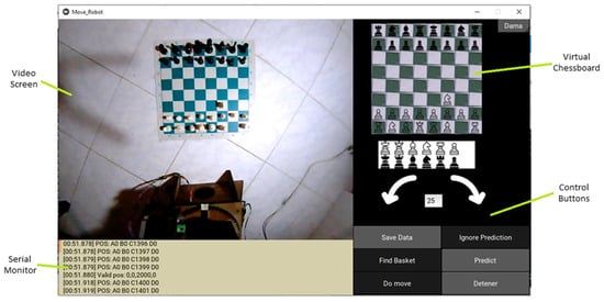
Figure 14.
Graphical user interface.
The components of the GUI are the following:
Video screen: Displays the video input of the fisheye camera, as well as the target point and cues during the visual servoing.
Serial monitor: Prints the commands received from the Arduino Mega.
Virtual board: Shows the progress during the game. It can also be manually edited to tag the images during the training database creation.
Control panel: Incorporates buttons to start a game, makes predictions of the colors of pieces, saves tagged images to the database, moves the arm manually, etc.
3. Results and Discussion
The integration of the mechanical and artificial vision systems resulted in a fully functional robot capable of autonomously playing chess against a human using Stockfish as a chess engine (see Figure 15). The mechanical system is currently used by the research group “Magma Ingeniería” to evaluate intelligent controllers using neural networks, fuzzy logic, and numeric optimization algorithms.
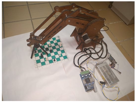
Figure 15.
Robotic arm.
3.1. Results for Capture and Image Processing
An example of the distorted image can be seen in Figure 16a, while the results obtained with the corrected image are shown in Figure 16b. The process consists of searching the corners of the chessboard squares and making an image database that is used to create a distortion correction matrix (see Figure 16c).
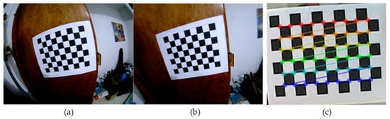
Figure 16.
(a) Example of a distorted image. (b) Corrected image. (c) Corner detection on the calibration chessboard.
Although the corrected image has a cutout space compared to the distorted image, the utility of the fisheye camera is demonstrated in comparison to a traditional 45-degree camera.
3.2. Chessboard Detection and Segmentation of the Squares
With the use of the Canny filter and the Hough transform, straight lines were detected on the board, which were filtered successfully using the Kernel density estimation. In this way, the peaks of the density function were interpreted as local averages in space to predict the positions of the lines on the board (see Figure 17).
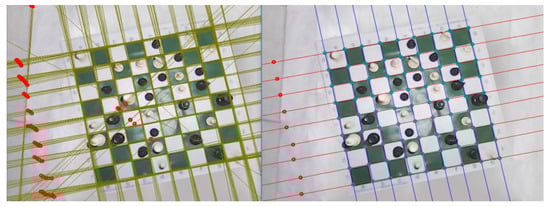
Figure 17.
Results obtained with the Hough transform and the Canny filter.
When lighting conditions are bad, this is the first stage in the image processing pipeline that fails. When the pieces create too many shadows on the board, the Hough transform may fail to recognize the lines.
3.3. Recognition Models
Different recognition models were evaluated, including logistic regression, a dense network, and a convolutional network. The best performance was obtained with the convolutional neural networks.
Logistic Regression: Six logistic regression models were implemented, one for each class label, achieving 93.1% accuracy for the test data.
Dense Network: The tested model consisted of 50 ReLU (Rectified Linear Unit) neurons in the hidden layer and 6 sigmoid output neurons, one for each class label. With this model, an accuracy of 94.4% was achieved for the test data. The improvement in performance was less than expected.
Convolutional Network: Two convolutional layers were implemented. The first layer had 32 filters and the second had 64 filters, using batch normalization and a dropout value of 20%. A dense layer with 6 outputs with sigmoidal activation was used, one for each classification label. Accuracy of 98.6% was achieved for the test data. This network was used as the basis for the Siamese network.
In the confusion matrix of the final model (See Figure 18), there were no errors in color predictions, but during the last training epochs, the precision ranged between 0.99 and 1.
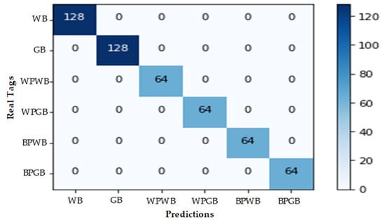
Figure 18.
Confusion matrix. Tags: white background (WB), green background (GB), white piece on white background (WPWB), white piece on green background (WPGB), black piece on white background (BPWB), and black piece on green background (BPGB).
Figure 19 shows that there is a region between epochs 30 and 100 where the model seems to over-fit and its performance falls for the test data; however, the model subsequently stabilizes and the curves overlap.
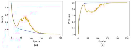
Figure 19.
(a) Losses vs. training epochs. (b) Precision vs. training epochs.
On the other hand, the success rate for detecting changes in the position of the chess pieces was 509/512. For all implemented models, because of the lack of color contrast, the most frequent confusions were presented in the following cases: (a) white piece on white background; (b) white background without a piece.
3.4. Manipulation
The four-finger gripper (see Figure 3) was specially designed for this project. The camera is positioned in the middle of the grip, making it is easy to center the end effector over the pieces. The disadvantage of this configuration is that if the camera is covered when a piece is grasped, then the image based visual servo can be used for the picking action, but not during the placement of the piece. Instead, the robot uses the IBVS to search the final position of the movement before grasping the piece, and later returns to the same coordinates.
Given the low-cost nature of the project and the simple open-loop mechanical system, the robot does not have good repeatability. When it blindly returns to a previous position to place a piece, there is 30% chance (15 out of 50 recorded movements) of placing the piece slightly over a line of that square.
On the other hand, the pickup movement of the piece is not seriously affected by the low accuracy of the mechanical system, because the error displacement (see vector V, Figure 12) is computed with respect to the camera mounted on the end effector. Also, the four-finger gripper easily centers the pieces during the gripping process, even when they are not properly placed in the middle of the square. The pickup manipulation errors are relatively low.
The method proposed by Tomasi and Kanade [57] to find features is prone to finding corners (points whose gradient matrix has at least two large eigenvalues). The chessboard has multiple crossing lines that provide multiple good quality tracking features; therefore, the IBVS implementation based on the Lukas–Tomasi–Kanade tracker works very well in this scenario.
4. Conclusions
A machine learning model for the color classification and movement detection of chess pieces was successfully implemented for the game perception of an autonomous chess-playing robot. Convolutional neural networks are suitable for the recognition of objects with low color contrast; such is the case for white pieces on white squares. The output feature vector of a convolutional neural network stage can be used at the same time for class classification and for detection of changes.
A fisheye camera attached to the gripper of a robot can be used successfully for visual servoing and object manipulation using the Kanade–Lucas–Tomasi algorithm, but problems can arise when moving blindly to previous positions if the robot mechanism has repeatability problems.
Author Contributions
C.d.T. performed the arm design and programming of the artificial vision system. C.R.-A. designed the experiments and wrote the manuscript. O.R.-Á. performed the data analysis and the revision and editing of the manuscript.
Funding
This research was funded by Vicerrectoría de Investigación of the Universidad del Magdalena.
Conflicts of Interest
The authors declare no conflict of interest.
References
- Kovacs, G.; Petunin, A.; Ivanko, J.; Yusupova, N. From the First Chess-Automaton to the Mars Pathfinder. Acta Polytech. Hung. 2016, 13, 61–81. [Google Scholar]
- Crandall, J.W.; Oudah, M.; Tennom; Ishowo-Oloko, F.; Abdallah, S.; Bonnefon, J.F.; Cebrian, M.; Shariff, A.; Goodrich, M.A.; Rahwan, I. Cooperating with machines. Nat. Commun. 2018, 9, 233. [Google Scholar] [CrossRef] [PubMed]
- Reconstructing Turing’s “Paper Machine”. Available online: https://en.chessbase.com/post/reconstructing-turing-s-paper-machine (accessed on 5 September 2019).
- Van den Herik, H.J. Computer chess: From idea to DeepMind. ICGA J. 2018, 40, 160–176. [Google Scholar] [CrossRef]
- Chakraborty, S.; Bhojwani, R. Artificial intelligence and human rights: Are they convergent or parallel to each other? Novum Jus 2018, 12, 13–38. [Google Scholar] [CrossRef]
- Castellano, G.; Leite, I.; Paiva, A. Detecting perceived quality of interaction with a robot using contextual features. Auton. Robot. 2017, 41, 1245–1261. [Google Scholar] [CrossRef]
- Dehghani, H.; Babamir, S.M. A GA based method for search-space reduction of chess game-tree. Appl. Intell. 2017, 47, 752–768. [Google Scholar] [CrossRef]
- Huang, M.-B.; Huang, H.-P. Innovative human-like dual robotic hand mechatronic design and its chess-playing experiment. IEEE Access 2019, 7, 7872–7888. [Google Scholar] [CrossRef]
- Lukač, D. Playing chess with the assistance of an industrial robot. In Proceedings of the 3rd International Conference on Control and Robotics Engineering, Nagoya, Japan, 20–23 April 2018; pp. 1–5. [Google Scholar] [CrossRef]
- Anh, N.D.; Nhat, L.T.; Van Phan Nhan, T. Design and control automatic chess-playing robot arm. Lect. Notes Electr. Eng. 2016, 371, 485–496. [Google Scholar] [CrossRef]
- Wei, Y.-A.; Huang, T.-W.; Chen, H.-T.; Liu, J. Chess recognition from a single depth image. In Proceedings of the IEEE International Conference on Multimedia and Expo, Hong Kong, China, 10–14 July 2017; pp. 931–936. [Google Scholar] [CrossRef]
- Larregay, G.; Pinna, F.; Avila, L.; Moran, D. Design and Implementation of a Computer Vision System for an Autonomous Chess-Playing Robot. J. Comput. Sci. Technol. 2018, 18, 1–11. [Google Scholar] [CrossRef]
- Xie, Y.; Tang, G.; Hoff, W. Chess Piece Recognition Using Oriented Chamfer Matching with a Comparison to CNN. In Proceedings of the IEEE Winter Conference on Applications of Computer Vision, Lake Tahoe, NV, USA, 12–15 March 2018; pp. 2001–2009. [Google Scholar] [CrossRef]
- Czyzewski, M.A.; Laskowski, A.; Wasik, S. Chessboard and chess piece recognition with the support of neural networks. Comput. Vis. Image Underst. 2018, 2, 1–11. [Google Scholar]
- Al-Saedi, F.A.T.; Mohammed, A.H. Design and Implementation of Chess-Playing Robotic System. IJCSET 2015, 5, 90–98. [Google Scholar]
- Mahmood, N.H.; Long, C.K.M.S.C.K. Smart Electronic Chess Board Using Reed Switch. J. Teknol. 2011, 55, 41–52. [Google Scholar] [CrossRef][Green Version]
- Larregay, G.; Avila, L.; Moran, O. A comparison of classification algorithms for chess pieces detection. In Proceedings of the 17th Workshop on Information Processing and Control, Mar del Plata, Argentina, 20–22 October 2017; pp. 1–5. [Google Scholar] [CrossRef]
- Ómarsdóttir, F.Y.; Ólafsson, R.B.; Foley, J.T. The Axiomatic Design of Chessmate: A Chess-playing Robot. Procedia CIRP 2016, 53, 231–236. [Google Scholar] [CrossRef][Green Version]
- Pachtrachai, K.; Vasconcelos, F.; Dwyer, G.; Pawar, V.; Hailes, S.; Stoyanov, D. CHESS-Calibrating the Hand-Eye Matrix with Screw Constraints and Synchronization. IEEE Robot. Autom. Lett. 2018, 3, 2000–2007. [Google Scholar] [CrossRef]
- Luqman, H.M.; Zaffar, M. Chess Brain and Autonomous Chess Playing Robotic System. In Proceedings of the International Conference on Autonomous Robot Systems and Competitions, Braganca, Portugal, 4–6 May 2016; pp. 211–216. [Google Scholar] [CrossRef]
- Wang, X.; Chen, Q. Vision-based entity Chinese chess playing robot design and realization. In International Conference on Intelligent Robotics and Applications; Springer: Cham, Switzerland, 2015; Volume 9246, pp. 341–351. [Google Scholar] [CrossRef]
- Chen, B.; Xiong, C.; Zhang, Q. CCDN: Checkerboard corner detection network for robust camera calibration. In International Conference on Intelligent Robotics and Applications; Springer: Cham, Switzerland, 2018; Volume 10985, pp. 324–334. [Google Scholar] [CrossRef]
- Kumar, R.V.Y. Target following Camera System Based on Real Time Recognition and Tracking. Master’s Thesis, National Institute of Technology, Rourkela, India, May 2014. [Google Scholar]
- Bennett, S.; Lasenby, J. ChESS-Quick and robust detection of chess-board features. Comput. Vis. Image Underst. 2014, 118, 197–210. [Google Scholar] [CrossRef]
- Matuszek, C.; Mayton, B.; Aimi, R.; Deisenroth, M.P.; Bo, L.; Chu, R.; Kung, M.; Le Grand, L.; Smith, J.R.; Fox, D. Gambit: An autonomous chess-playing robotic system. In Proceedings of the IEEE International Conference on Robotics and Automation, Seattle, WA, USA, 9–13 May 2011; pp. 4291–4297. [Google Scholar] [CrossRef]
- Koray, C.; Sümer, E. A Computer Vision System for Chess Game Tracking. In Proceedings of the 21st Computer Vision Winter Workshop, Rimske Toplice, Slovenia, 3–5 February 2016; pp. 1–7. [Google Scholar]
- Christie, D.A.; Kusuma, T.M.; Musa, P. Chess piece movement detection and tracking, a vision system framework for autonomous chess playing robot. In Proceedings of the 2nd International Conference on Informatics and Computing, Papua, Indonesia, 1–3 November 2017; pp. 1–6. [Google Scholar] [CrossRef]
- Chen, A.T.-Y.; Wang, K.I.-K. Robust Computer Vision Chess Analysis and Interaction with a Humanoid Robot. Computers 2019, 8, 14. [Google Scholar] [CrossRef]
- Yıldız, İ.; Tian, P.; Dy, J.; Erdoğmuş, D.; Brown, J.; Kalpathy-Cramer, J.; Ostmo, S.; Peter Campbell, J.; Chiang, M.F.; Ioannidis, S. Classification and comparison via neural networks. Neural Netw. 2019, 118, 65–80. [Google Scholar] [CrossRef]
- Sun, W.-T.; Chao, T.-H.; Kuo, Y.-H.; Hsu, W.H. Photo Filter Recommendation by Category-Aware Aesthetic Learning. IEEE Trans. Multimed. 2017, 19, 1870–1880. [Google Scholar] [CrossRef]
- Shi, H.B.; Chen, J.L.; Pan, W.; Hwang, K.S.; Cho, Y.Y. Collision Avoidance for Redundant Robots in Position-Based Visual Servoing. IEEE Syst. J. 2019, 13, 3479–3489. [Google Scholar] [CrossRef]
- Pairo, W.; Loncomilla, P.; Del Solar, J.R. A Delay-Free and Robust Object Tracking Approach for Robotics Applications. J. Intell. Robot. Syst. 2019, 95, 99–117. [Google Scholar] [CrossRef]
- Kim, S.; Seo, H.; Choi, S.; Kim, H.J. Vision-Guided Aerial Manipulation Using a Multirotor With a Robotic Arm. IEEE-ASME Trans. Mechatron. 2016, 21, 1912–1923. [Google Scholar] [CrossRef]
- Beckerle, P.; Bianchi, M.; Castellini, C.; Salvietti, G. Mechatronic designs for a robotic hand to explore human body experience and sensory-motor skills: A Delphi study. Adv. Robot. 2018, 32, 670–680. [Google Scholar] [CrossRef]
- Robles, C.A.; Román Ortega, D.J.; Polo Llanos, A.M. Design of an eighteen degrees-of-freedom robotic arm with teleoperation by an electronic glove [Brazo robótico con dieciocho grados de libertad tele-operado por un guante electrónico]. Espacios 2017, 38, 22. [Google Scholar]
- Robles-Algarín, C.; Echavez, W.; Polo, A. Printed Circuit Board Drilling Machine Using Recyclables. Electronics 2018, 7, 240. [Google Scholar] [CrossRef]
- Covaciu, F.; Filip, D. Design and Manufacturing of A 6 Degree of Freedom Robotic Arm. Acta Tech. Napoc. Ser.-Appl. Math. Mech. Eng. 2019, 62, 107–114. [Google Scholar]
- Timoftei, S.; Brad, E.; Sarb, A.; Stan, O. Open-Source Software in Robotics. Acta Tech. Napoc. Ser.-Appl. Math. Mech. Eng. 2018, 61, 519–526. [Google Scholar]
- Safin, R.; Lavrenov, R.; Martinez-Garcia, E.A.; Magid, E. ROS-based Multiple Cameras Video Streaming for a Teleoperation Interface of a Crawler Robot. J. Robot. Netw. Artif. Life 2018, 5, 184–189. [Google Scholar] [CrossRef]
- Rosa, S.; Toscana, G.; Bona, B. Q-PSO: Fast Quaternion-Based Pose Estimation from RGB-D Images. J. Intell. Robot. Syst. 2018, 92, 465–487. [Google Scholar] [CrossRef]
- Lin, J.P.; Guo, T.L.; Yan, Q.F.; Wang, W.X. Image segmentation by improved minimum spanning tree with fractional differential and Canny detector. J. Algorithms Comput. Technol. 2019, 13. [Google Scholar] [CrossRef]
- Wu, G.H.; Yang, D.Y.; Chang, C.; Yin, L.F.; Luo, B.; Guo, H. Optimizations of Canny Edge Detection in Ghost Imaging. J. Korean Phys. Soc. 2019, 75, 223–228. [Google Scholar] [CrossRef]
- Mazhar, O.; Navarro, B.; Ramdani, S.; Passama, R.; Cherubini, A. A real-time human-robot interaction framework with robust background invariant hand gesture detection. Robot. Comput. Integr. Manuf. 2019, 60, 34–48. [Google Scholar] [CrossRef]
- Winterhalter, W.; Fleckenstein, F.V.; Dornhege, C.; Burgard, W. Crop Row Detection on Tiny Plants with the Pattern Hough Transform. IEEE Robot. Autom. Lett. 2018, 3, 3394–3401. [Google Scholar] [CrossRef]
- Banerjee, D.; Yu, K.; Aggarwal, G. Object Tracking Test Automation Using a Robotic Arm. IEEE Access 2018, 6, 56378–56394. [Google Scholar] [CrossRef]
- Alzarok, H.; Fletcher, S.; Longstaff, A.P. 3D Visual Tracking of an Articulated Robot in Precision Automated Tasks. Sensors 2017, 17, 104. [Google Scholar] [CrossRef]
- Paulo, J.; Asvadi, A.; Peixoto, P.; Amorim, P. Human gait pattern changes detection system: A multimodal vision-based and novelty detection learning approach. Biocybern. Biomed. Eng. 2017, 37, 701–717. [Google Scholar] [CrossRef]
- Costa, M.A.; Wullt, B.; Norrlof, M.; Gunnarsson, S. Failure detection in robotic arms using statistical modeling, machine learning and hybrid gradient boosting. Measurement 2019, 146, 425–436. [Google Scholar] [CrossRef]
- Janke, J.; Castelli, M.; Popovic, A. Analysis of the proficiency of fully connected neural networks in the process of classifying digital images. Benchmark of different classification algorithms on high-level image features from convolutional layers. Expert Syst. Appl. 2019, 135, 12–38. [Google Scholar] [CrossRef]
- Lu, Z.C.; Yeung, H.W.F.; Qu, Q.; Chung, Y.Y.; Chen, X.M.; Chen, Z.B. Improved image classification with 4D light-field and interleaved convolutional neural network. Multimed. Tools Appl. 2019, 78, 29211–29227. [Google Scholar] [CrossRef]
- Seo, J.H.; Kwon, D.S. Learning 3D local surface descriptor for point cloud images of objects in the real-world. Robot. Auton. Syst. 2019, 116, 64–79. [Google Scholar] [CrossRef]
- Kuai, Y.L.; Wen, G.J.; Li, D.D. Masked and dynamic Siamese network for robust visual tracking. Inf. Sci. 2019, 503, 169–182. [Google Scholar] [CrossRef]
- Liu, X.N.; Zhou, Y.; Zhao, J.Q.; Yao, R.; Liu, B.; Zheng, Y. Siamese Convolutional Neural Networks for Remote Sensing Scene Classification. IEEE Geosci. Remote Sens. 2019, 16, 1200–1204. [Google Scholar] [CrossRef]
- Yang, K.; Song, H.H.; Zhang, K.H.; Fan, J.Q. Deeper Siamese network with multi-level feature fusion for real-time visual tracking. Electron. Lett. 2019, 55, 742–744. [Google Scholar] [CrossRef]
- Cheng, C.A.; Huang, H.P.; Hsu, H.K.; Lai, W.Z.; Cheng, C.C. Learning the Inverse Dynamics of Robotic Manipulators in Structured Reproducing Kernel Hilbert Space. IEEE Trans. Cybern. 2016, 46, 1691–1703. [Google Scholar] [CrossRef] [PubMed]
- Ci, W.Y.; Huang, Y.P. A Robust Method for Ego-Motion Estimation in Urban Environment Using Stereo Camera. Sensors 2016, 16, 1704. [Google Scholar] [CrossRef] [PubMed]
- Tomasi, C.; Kanade, T. Detection and Tracking of Point Features. Int. J. Comput. Vis. 1991, 9, 137–154. [Google Scholar] [CrossRef]


© 2019 by the authors. Licensee MDPI, Basel, Switzerland. This article is an open access article distributed under the terms and conditions of the Creative Commons Attribution (CC BY) license (http://creativecommons.org/licenses/by/4.0/).