A Deep Learning Method for 3D Object Classification Using the Wave Kernel Signature and A Center Point of the 3D-Triangle Mesh

Abstract

Computer vision recently has many applications such as smart cars, robot navigation, and computer-aided manufacturing. Object classification, in particular 3D classification, is a major part of computer vision. In this paper, we propose a novel method, wave kernel signature (WKS) and a center point (CP) method, which extracts color and distance features from a 3D model to tackle 3D object classification. The motivation of this idea is from the nature of human vision, which we tend to classify an object based on its color and size. Firstly, we find a center point of the mesh to define distance feature. Secondly, we calculate eigenvalues from the 3D mesh, and WKS values, respectively, to capture color feature. These features will be an input of a 2D convolution neural network (CNN) architecture. We use two large-scale 3D model datasets: ModelNet10 and ModelNet40 to evaluate the proposed method. Our experimental results show more accuracy and efficiency than other methods. The proposed method could apply for actual-world problems like autonomous driving and augmented/virtual reality.

1. Introduction

Recently, computer vision has achieved great results along the development of computer hardware. Also, we can build highly complex systems, for example, autonomous driving, by applying the deep learning for solving computer vision task. A self-driving car needs to recognize objects on the street, for example, people or another car, which leads to the necessity of 3D object classification [1].

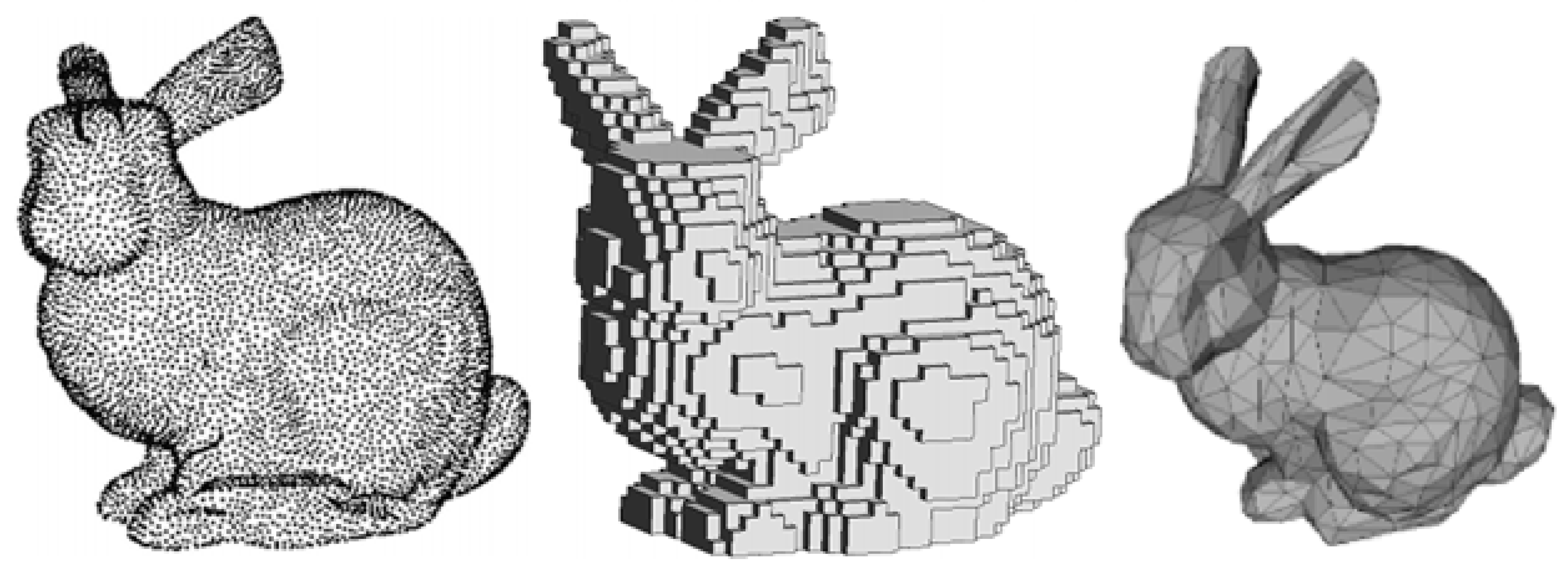
The 3D classification remains a challenge for researchers in this field. In the past, we had only 2D classification or 2D image classification due to the limit of 3D resources and computer hardware. The technology of 3D acquisition such as Microsoft Kinect recently produces a massive amount of 3D-data and boosts 3D classification. 3D systems are more complicated than 2D systems due to some reasons: Data representation, different distributions of objects [2]. Main problems are that 3D systems require more hardware resources as well as the computation time for the additional dimension.

Non-machine learning methods present the worst results on 3D object classification, lower than 76% accuracy for dataset: ModelNet40 [3,4]. Advancements in deep learning allow us to propose convolution neural network (CNN)-based methods in solving the traditional methods’ drawbacks in 3D classification. There are two CNN structures for various 3D-data representation: 2D CNN for multi-view and point cloud, 3D CNN for voxel. Currently, 2D CNN has a complete architecture with great results while 3D CNN is still under improvement [5].

We aim to introduce a new method, center point (CP) and wave kernel signature (WKS) method, for 3D object classification. In the next section, we present related works of 3D object classification. Section 3 presents a description of the proposed method; Section 4 shows the experimental results and the comparison with other methods. The conclusion will be given in Section 5.

2. Related Works

2.1. 3D Data Representation

The first 3D data form is point cloud, which is the collection of points in space. Each point has only one value of (x, y, z) in a 3D-Cartesian coordinate system and other properties such as color values [6]. The second 3D data form is voxel. Voxels are like volume pixels in three-dimensional space, which is a 3D version of a pixel in a 2D image [7]. The last 3D-data form is a 3D-triangle mesh. Unlike the point cloud and voxel, this mesh is constructed from 3D-triangle facets with three vertices for each facet. The 3D triangle mesh is more popular than other forms of 3D data because it is user-friendly [8]. Figure 1 displays different data representation of the same 3D object [9,10,11].

2.2. 3D Shape Analysis

The most important property of a 3D-object is its shape. The main object of shape analysis is to find differences between the shapes of a 3D model. We use descriptors to store location information of the 3D model. WKS is a method to obtain descriptors based on quantum mechanics at specific locations. WKS shows energy distributions on different boundaries of the 3D object [12]. WKS maps one point in space ${\mathrm{R}}^3$ to feature space ${\mathrm{R}}^{\mathrm{N}}$ which stores the local and global information about that point. The low frequency and the high-frequency represent the global feature and the local feature, respectively [13]. Accessing high-frequency information, WKS will be suitable for 3D object matching [14]. Figure 2 shows an example of WKS for a 3D object.

2.3. 3D Object Classification

3D object classification is an everlasting research area that developed various techniques dependent on local and global shape descriptors in earlier times [15]. Several studies have proposed some different AI techniques such as CNN, which helped to solve many 2D classification problems completely. It is reasonable to extend well-known results of CNN on 2D images problems to similar applications on 3D data.

It is incredibly hard to directly use CNN for 3D object classification because 3D data structures are more complicated than regular formats of 2D data. The solution is to transform 3D objects into data forms that work with the input layer of CNN. As a result, methods for representations of 3D shapes divide into two following main types.

Firstly, Voxelization-based methods, volume pixel in 3D space, provide a detailed description of an object and adapt 3D CNNs to the voxel structure. Wu et al. [16] used a convolutional deep belief network to express input shapes as the probability of extending on 3D voxel grids while the PointNet method [17] uses the occupation grids that work with the input layer of CNN for classifying 3D shapes.

Secondly, projection-based methods, which present 3D objects into different 2D-spaces, depend on the idea of drawing 3D objects from various viewpoints, then take captured images and insert it to the input layer of CNN. Reference [18] uses a spherical parameterization to display the 3D mesh in a geometry-image, which encloses inflection information for the input of CNN. The authors in [19] recommend representing 3D objects with a panoramic view.

3. Methodology

Color and spatial are two popular and necessary features in 2D image classification [20,21]. For the 3D objects, we use the WKS to capture the color feature and a CP to get the spatial feature, specifically the distance feature. We use the color feature for the 3D object classification because the color feature is the most popular and necessary property in the mechanism of human visual perception, and it is easy to analyze the color. Similarly, we use the distance feature due to its importance for the 3D object classification in giving information on the structural arrangement of the 3D objects. The basic primitives define the distance feature. The spatial distribution of basic primitives creates some visual forms, which are defined by directionality, repetitiveness, and granularity. Therefore, we combine the color and distance features to get higher performance in 3D object classification.

Figure 3 shows two main stages of the proposed method. In the first stage, we find a center point of a 3D mesh and choose N random vertices from this mesh. Then, we calculate and store the distance from this center point to each vertex in the first 3D-matrix. The second stage is that we calculate and store WKS values of a 3D mesh into the second 3D-matrix. Those values define the color of the 2D projection construction of the model. The combination of those two matrices forms a 6D-matrix for the input of 2D CNN. The sub-sections below give a detailed description of the proposed method.

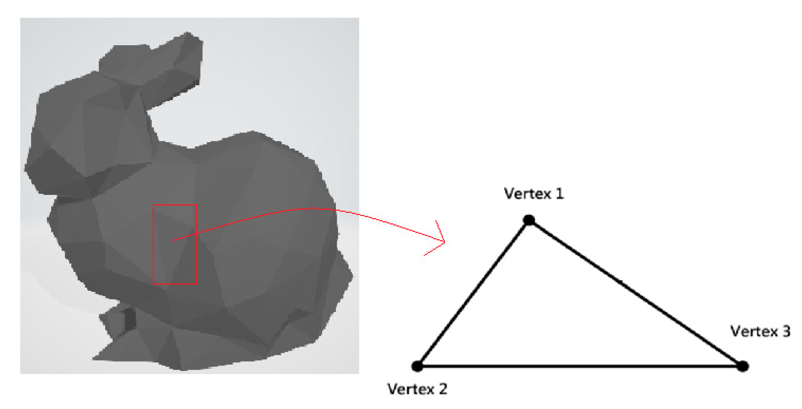
Our method is based on the 3D triangle mesh with one or more triangles. According to Figure 4, the location of three vertices defines each triangle (called a facet).

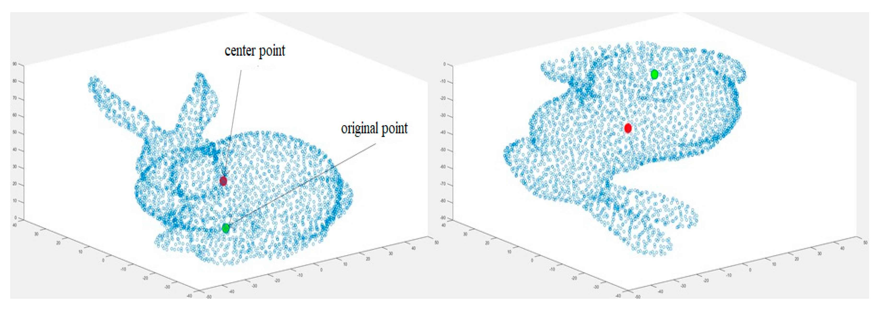
3.1. The Center Point of 3D Triangle Mesh (CP)

We find a center point of a 3D model, consisting of a collection of M vertices, having coordinates ${\mathrm{V}}_{\mathrm{i}}\left({\mathrm{x}}_{\mathrm{i}},{\mathrm{y}}_{\mathrm{i}},{\mathrm{z}}_{\mathrm{i}}\right)$ (i=1: M).

The following equation determines the center point C, having coordinates (${\mathrm{C}}_{\mathrm{x}},{\mathrm{C}}_{\mathrm{y}},{\mathrm{C}}_{\mathrm{z}})$:

$$\mathrm{C}=\frac{1}{M}{{\displaystyle \sum }}_{\mathrm{i}=1}^M{\mathrm{V}}_{\mathrm{i}}$$

(1)

We calculate the distance ${\mathrm{D}}_{{\mathrm{x}}_{\mathrm{i}}},{\mathrm{D}}_{{\mathrm{y}}_{\mathrm{i}}},{\mathrm{D}}_{{\mathrm{z}}_{\mathrm{i}}}$ from M vertices to the center point:

$${\mathrm{D}}_{{\mathrm{x}}_{\mathrm{i}}}={\mathrm{x}}_{\mathrm{i}}-{\mathrm{C}}_{\mathrm{x}},$$

$${\mathrm{D}}_{{\mathrm{y}}_{\mathrm{i}}}={\mathrm{y}}_{\mathrm{i}}-{\mathrm{C}}_{\mathrm{y}},$$

(2)

$${\mathrm{D}}_{{\mathrm{z}}_{\mathrm{i}}}={\mathrm{z}}_{\mathrm{i}}-{\mathrm{C}}_{\mathrm{z}}.$$

D_max is defined by

$${\mathrm{D}}_{\max }=\max (\{{\mathrm{D}}_{{\mathrm{x}}_{\mathrm{i}}},{\mathrm{D}}_{{\mathrm{y}}_{\mathrm{i}}},{\mathrm{D}}_{{\mathrm{z}}_{\mathrm{i}}}|\mathrm{i}=1:M\}).$$

(3)

We choose N = 1024 random vertices from M vertices of the 3D mesh, and we replace missing values by zero in case of M < 1024. We obtain N × 3 values for constructing a 3D-matrix. We re-shape each dimension from 1024 to a 32 by 32 matrix and obtain a final 32 by 32 by 3 matrix, ${\mathrm{A}}_1$, in which the x-axis and y-axis represent the first two dimensions; the z-axis, the third dimension.

We will normalize the distance values in the range from −1 to 1 so that the 3D model fits into a sphere unit. We divide all current elements in matrix ${\mathrm{A}}_1$ by the maximum value ${\mathrm{D}}_{\max }$ (3) of the 3D model.

Then the normalized values of matrix A will be calculated as:

$$\mathrm{A}=\frac{{\mathrm{A}}_1}{{\mathrm{D}}_{\max }}.$$

(4)

Given the Figure 5, we obtain the same values of matrix A when rotating the model by 180 degrees, so the rotation of a 3D model produces the consistent final matrix A.

3.2. Wave Kernel Signature on the 3D Triangle Mesh (WKS)

We first derive a Laplacian matrix from a 3D mesh, then calculate its eigenvalues and eigenvectors [22]. By modifying Equation (10) in [14], each ${\mathrm{WKS}}_{\mathrm{i}}$ value for a vertex ${\mathrm{V}}_{\mathrm{i}}$ is calculated as:

$${\mathrm{WKS}}_{\mathrm{i}}={\displaystyle \sum }_{\mathrm{k}=1}^{\mathrm{S}}{\varnothing }_{\mathrm{ik}}^2\left({\mathrm{V}}_{\mathrm{i}}\right){\mathrm{e}}^{-\frac{{\left(\mathrm{e}-\mathrm{logE}\left(\mathrm{k}\right)\right)}^2}{2{\mathsf{\sigma }}^2}}.$$

(5)

Formula (5) can be written clearly, as follow:

$$\{\begin{array}{c}{\mathrm{WKS}}_1={\displaystyle \sum }_{\mathrm{k}=1}^{\mathrm{S}}{\varnothing }_{1\mathrm{k}}^2\left({\mathrm{V}}_1\right){\mathrm{e}}^{-\frac{{\left(\mathrm{e}-\mathrm{logE}\left(\mathrm{k}\right)\right)}^2}{2{\mathsf{\sigma }}^2}},\\ {\mathrm{WKS}}_2={\displaystyle \sum }_{\mathrm{k}=1}^{\mathrm{S}}{\varnothing }_{2\mathrm{k}}^2\left({\mathrm{V}}_2\right){\mathrm{e}}^{-\frac{{\left(\mathrm{e}-\mathrm{logE}\left(\mathrm{k}\right)\right)}^2}{2{\mathsf{\sigma }}^2}},\\ ⋮\\ {\mathrm{WKS}}_M={\displaystyle \sum }_{\mathrm{k}=1}^{\mathrm{S}}{\varnothing }_{\mathrm{Mk}}^2\left({\mathrm{V}}_M\right){\mathrm{e}}^{-\frac{{\left(\mathrm{e}-\mathrm{logE}\left(\mathrm{k}\right)\right)}^2}{2{\mathsf{\sigma }}^2}}.\end{array}$$

Equivalently,

$$\{\begin{array}{c}{\mathrm{WKS}}_1={\varnothing }_{11}^2\left({\mathrm{V}}_1\right){\mathrm{e}}^{-\frac{{\left(\mathrm{e}-\mathrm{logE}\left(1\right)\right)}^2}{2{\mathsf{\sigma }}^2}}+{\varnothing }_{12}^2\left({\mathrm{V}}_1\right){\mathrm{e}}^{-\frac{{\left(\mathrm{e}-\mathrm{logE}\left(2\right)\right)}^2}{2{\mathsf{\sigma }}^2}}+\cdots +{\varnothing }_{1S}^2\left({\mathrm{V}}_1\right){\mathrm{e}}^{-\frac{{\left(\mathrm{e}-\mathrm{logE}\left(\mathrm{S}\right)\right)}^2}{2{\mathsf{\sigma }}^2}},\\ {\mathrm{WKS}}_2={\varnothing }_{21}^2\left({\mathrm{V}}_2\right){\mathrm{e}}^{-\frac{{\left(\mathrm{e}-\mathrm{logE}\left(1\right)\right)}^2}{2{\mathsf{\sigma }}^2}}+{\varnothing }_{22}^2\left({\mathrm{V}}_2\right){\mathrm{e}}^{-\frac{{\left(\mathrm{e}-\mathrm{logE}\left(2\right)\right)}^2}{2{\mathsf{\sigma }}^2}}+\cdots +{\varnothing }_{2S}^2\left({\mathrm{V}}_2\right){\mathrm{e}}^{-\frac{{\left(\mathrm{e}-\mathrm{logE}\left(\mathrm{S}\right)\right)}^2}{2{\mathsf{\sigma }}^2}},\\ ⋮\\ {\mathrm{WKS}}_M={\varnothing }_{M1}^2\left({\mathrm{V}}_M\right){\mathrm{e}}^{-\frac{{\left(\mathrm{e}-\mathrm{logE}\left(1\right)\right)}^2}{2{\mathsf{\sigma }}^2}}+{\varnothing }_{M2}^2\left({\mathrm{V}}_M\right){\mathrm{e}}^{-\frac{{\left(\mathrm{e}-\mathrm{logE}\left(2\right)\right)}^2}{2{\mathsf{\sigma }}^2}}+\cdots +{\varnothing }_{MS}^2\left({\mathrm{V}}_M\right){\mathrm{e}}^{-\frac{{\left(\mathrm{e}-\mathrm{logE}\left(\mathrm{S}\right)\right)}^2}{2{\mathsf{\sigma }}^2}}.\end{array}$$

S = 300 is the number of eigenvalues; E is a Sx1 vector of eigenvalues; M is the number of vertices of the 3D mesh; $\varnothing =\left[\begin{array}{cccc}{\varnothing }_{11}\left(V_1\right)& {\varnothing }_{12}\left(V_1\right)& \cdots & {\varnothing }_{1S}\left(V_1\right)\\ ⋮& ⋮& \ddots & ⋮\\ {\varnothing }_{M1}\left(V_M\right)& {\varnothing }_{M2}\left(V_M\right)& \cdots & {\varnothing }_{MS}\left(V_M\right)\end{array}\right]$ is a MxS matrix of the corresponding eigenvectors.

Then the WKS feature vector of a 3D mesh is defined by:

$$\mathrm{WKS}=\left[\begin{array}{c}{\mathrm{WKS}}_1\\ {\mathrm{WKS}}_2\\ ⋮\\ {\mathrm{WKS}}_M\end{array}\right].$$

(6)

The variance $\mathsf{\sigma }$ is defined as

$$\mathsf{\sigma }=\frac{{\mathrm{e}}_{\max }-\mathrm{e}}{20},$$

(7)

where ${\mathrm{e}}_{\max }=\max \left(\mathrm{logE}\right),$ the logarithmic energy scale $\mathrm{e}=\mathrm{logE}\left(2\right),$ and E(2) is the second element of E.

We construct a colormap, based on the WKS feature vector. We have M vertices and M color values corresponding with the M values of WKS. Each value ${\mathrm{WKS}}_{\mathrm{i}}$ controls each value of vertex ${\mathrm{V}}_{\mathrm{i}}$, as shown in Figure 6.

In Figure 6, we suppose that the $M\mathrm{th}$ and the second vertex have the largest and the smallest values, namely WKSM and WKS2, which then are mapped to the last and the first row of the colormap, respectively.

After applying WKS to the 3D model, the black and white original model is changed into the color model. The second matrix B in a 32 by 32 by 3 pixel is used to capture and store a 2D projection of the 3D color model, as shown in Figure 7.

3.3. The Architecture of Convolution Neural Network

We obtain a 32 by 32 by 6 matrix C by concatenating A and B along the third dimension, then use matrix C for the input data of CNN. Figure 8 shows the architecture of the convolution neural network. As shown in Figure 8, a typical design, where an input layer is followed by four convolutional blocks and two fully connected layers, is used to build the convolutional neural network architecture selected in the proposed implementation. Each convolutional block consists of convolution, batch normalization, and rectified linear units (ReLUs). The corresponding number of filters for all convolution layers in each block are 16, 32, 64, and 128, respectively. The padding for the first and other convolutional blocks is to set values 1 and 0, respectively, and we assign value 3 to kernel size for all layers. The stride equals 2 in the last two convolution blocks and 1 in the first two convolution blocks. Then, we insert an 8 by 8 average pooling layer after the fourth convolution block. Batch normalizations and a dropout layer are used in our network for the following reasons.

Firstly, batch normalization has some advantages such as making predictions of network output more stable, accelerating training by magnitude order, and reducing overfitting through regularization. Batch normalization normalizes activations in a network across a mini-batch by subtracting the mean and dividing by the standard deviation of these activations. Normalization is necessary because some activations may be higher, which may cause subsequent layers abnormally, and make a less stable network even after normalizing input.

Secondly, we add a dropout layer between a pooling layer and a fully connected layer to improve convergence. This introduces a stochastic gradient descent (SGD) optimizer to reduce the cumulative error and to improve the training speed as well as to fix the overfitting problem due to an expansion in the number of iterations. Dropout is a mean model, which is the weighted average of estimation or prediction output from various models. The hidden layer nodes may be neglected from a random selection in the dropout. As a result, each training network is unique and is considered as a new model. Specifically, hidden nodes are likely to occur randomly. Updating weights do not base on the interaction of fixed nodes, and this avoids possible connections of some features with another specific feature because any two hidden nodes do not appear in models many times concurrently. Thus, we can ignore some nodes randomly in the network. Ignoring these hidden layer nodes can decrease calculation cost. Moreover, these ignored nodes can restrict other nodes from joining each other to decrease overfitting [23].

Matrix C enters the input layer in the first step of the whole process. Then, the first convolution block uses those data to apply a convolution function with a 1 by 1 stride. The output of the first convolution layer is 16 feature maps of dimension 32 by 32 which transfer to the first ReLU layer via the first batch normalization layer. Learning becomes faster with Gradient descent because the batch normalization renormalizes data. Sixteen normalized-features are the output of the first batch normalization layer. The second convolutional layer applies the convolution function with a 1 by 1 stride to the first ReLU layer’s output. This second layer’s output is 16 feature maps of dimension 32 by 32 which move to the second batch normalization layer and the second ReLU layer, respectively. We repeat the process until the fourth convolution block. The last output will be the input of the average pooling layer and dropout layer.

The first fully connected layer takes the dropout layer’s output, which has a feature vector with size 128, travels to the second fully connected layer. Then this second layer takes only K (K = 10 or 40) most active features and sends them to the softmax layer. Ten or forty classes with corresponding class names are used for classifying output such as the airplane, bed, and desk.

4. Experimental Results

To verify the proposed method, we use the most popular 3D dataset: The ModelNet, which has two sub-datasets: ModelNet10 and ModelNet40 [16]. The original ModelNet dataset can be downloaded from the website in the Supplementary Materials. ModelNet10 and ModelNet40 have 3D CAD models from 10 categories with 3991 training and 908 testing objects, and from 40 categories such as airplanes, bathtubs, beds, and benches with 9843 training and 2468 testing objects, respectively. Each object of ModelNet dataset has a format of a 3D-triangle mesh, namely OFF.

Table 1. The distribution of classes in the ModelNet10 dataset.

Class Name	Train	Test	Total
bathtub	106	50	156
bed	515	100	615
chair	889	100	989
desk	200	86	286
dresser	200	86	286
monitor	465	100	565
nightstand	200	86	286
sofa	680	100	780
table	392	100	492
toilet	344	100	444
total	3991	908	4899

shows the amount of objects of a particular class for dataset: ModelNet10.

We re-mesh objects in ModelNet or keep the original model without re-meshing if the number of vertices is larger or smaller than 3600, respectively. Some classes in the dataset such as glass-box have 171 models on the training folder; three models among them have more than 3600 vertices and the minimum number of vertices for one object is 44. As seen in Figure 9, there are not many differences between the original model and the re-meshed model because the shapes of the objects are still kept except unimportant information. The re-meshing process plays a role as the technology which we use in the image or audio compressing. It seems unable for a “normal” user to distinguish between the original wave sound and the MP3 sound compressed. We create a new dataset from the original Modelnet dataset by keeping the structure of the original dataset and applying the re-meshing process for some models. We can see some random objects in the new dataset in Figure 10. Applying the re-mesh process did not affect the accuracy of the method because it still keeps objects’ shapes, but reduces the number of vertices and faces. We apply the proposed method to find the distance and color feature of all 3D models after preprocessing the original dataset. All experiments were conducted on the machine i7 7700, 16GB memory, 1080Ti GPU, MATLAB (9.6 (R2019a), Natick, MA, USA).

We first read the OFF file of the model, store the information of each vertex. Suppose the number of vertices is M, and calculate M values of WKS. Then we plot the 3D model with the color depending on those WKS values. We also calculate the distance between the center point to each vertex in the 3D mesh of the OFF file. After having the information of distance and color, we combined distance and color values into a 32 by 32 by 6 matrix and put it into the proposed CNN architecture. We use SGD with the mini-batch size at 64, and the momentum at 0.9 to train the network, and divide the initial learning rate at 0.2 by half for all 160 epochs. As listed in

Table 2. The accuracy between the proposed method and other methods on the ModelNet dataset.

Algorithm	ModelNet10	ModelNet40
PointNet [17]	77.60%	N/A
3D ShapeNets [16]	83.54%	77.32%
Geometry Image [18]	88.40%	83.90%
DeepPano [19]	88.66%	82.54%
PanoramicView [24]	89.80%	82.47%
Our Method	90.20%	84.64%

, the proposed method has precision levels at 90.20% and 84.64% for ModelNet10 and ModelNet40, respectively, which is more accurate than other methods. Our methods had precision levels which were 7.32% and 6.66% higher than the deep learning method 3DShapeNets for 40 and 10 classes, respectively.

Both the DeepPano and Panoramic View method use four convolution Blocks, where each convolution Block contains one convolution layer, followed by one max pooling layer. In contrast, our method uses four convolution blocks, which each includes two same convolution layers, two batch normalization layers, and two ReLU layers. The number of parameters is greater than 0 in the pooling layer while it equals 0 in batch normalization and ReLU layer.

The authors in [19] did not mention numbers of feature vectors in their fully connected layer of the DeepPano method, hence we compare the number of parameters in the convolution layers, not in fully connected layers. We use two fully connected layers with 128 and K (K = 10 or K = 40) feature vectors, respectively, in our method instead of using 512 and 1024 feature vectors for the first and the second layer as mentioned in the panoramic view method. Considering the results in

Table 3. The total number of parameters for all convolution layers in different methods.

Layers	DeepPano	Parameters	PanoView	Parameters	Our Method	Parameters
Input	160 × 64	0	108 × 36	0	32 × 32 × 6	0
Conv1	(5, 96)	2496	(1, 64)	128	Two (3, 16)	320
Conv2	(5, 256)	6656	(2, 80)	400	Two (3, 32)	640
Conv3	(3, 384)	3840	(4, 160)	2720	Two (3, 64)	1280
Conv4	(3, 512)	5120	(6, 320)	11,840	Two (3, 128)	2560
FC1	N. Available	N. Available	512	N. Available	128	N. Available
FC2	N. Available	N. Available	1024	N. Available	10 or 40	N. Available
Total		18,112		15,088		4800

, our methods used fewer parameters for all convolution layers than their methods. Our method used 4800 parameters in total, compared with 18,112 for DeepPano and 15,088 for panoramic view. It is generally to conclude that our method is more efficient due to the reduction of model parameters, diminishing the computational cost.

We plot a confusion matrix for the ModelNet40 in Figure 11. Flower Pot class and Plant class are the most misclassified, where 60% of the flower pot has miss-classification as the plant due to their similarities (see Figure 10).

As seen in

Table 4. The accuracy of each class in dataset: ModelNet10.

Class	PointNet	Our Method	Class	PointNet	Our Method
bathtub	34	39	monitor	87	100
bed	80	99	nightstand	60	63
chair	90	100	sofa	88	94
desk	52	67	table	69	80
dresser	61	77	toilet	84	100

, our methods had higher accuracy in the dataset: ModelNet10 due to the combination of color and distance features. In some classes, the distance feature will be complementary for the color feature. For example, in some cases, two objects in the dresser class have five similar faces and different the sixth face. The distance feature will help to recognize the spatial distribution of the model and improve the accuracy for classification. Specifically, PointNet can recognize 61 of 86 dresser models, while our method is 77 of 86.

Increasing the number of features will improve the accuracy of classification. Geometry Image method extracts only the color feature while our method uses the additional distance feature. Moreover, both DeepPano and panoramic view use only a view base without the spatial feature.

Wave kernel signature and center point achieved better accuracy due to the above reasons.

5. Conclusions

In this paper, we created an innovative approach for 3D object classification by combining two features: Color and distance. Our method has achieved more accuracy and efficiency than five other methods: PointNet, 3DShapeNets, geometry image, DeepPano, and panoramic view.

Classification is a crucial step for other tasks like object retrieval. Also, our method is consistent with the object rotation, so it is suitable for retrieval task. Future direction for research and development is to integrate the software into actual world problems like fully autonomous cars or manufacture factories.

References

1. Geiger, A.; Lenz, P.; Urtasun, R. Are we ready for autonomous driving? The kitti vision benchmark suite. In Proceedings of the 2012 IEEE Conference on Computer Vision and Pattern Recognition, Providence, RI, USA, 16–21 June 2012; pp. 3354–3361. [Google Scholar] [CrossRef]
2. Shen, X. A Survey of Object Classification and Detection Based on 2D/3D Data. Available online: https://arxiv.org/abs/1905.12683 (accessed on 20 September 2019).
3. Kazhdan, M.; Funkhouser, T.; Rusinkiewicz, S. Rotation invariant spherical harmonic representation of 3D shape descriptors. In Proceedings of the Eurographics/ACM SIGGRAPH Symposium on geometry processing, Aachen, Germany, 23–25 June 2003; pp. 156–164. [Google Scholar]
4. Chen, D.-Y.; Tian, X.-P.; Shen, Y.-T.; Ouhyoung, M. On visual similarity based 3D model retrieval. Comput. Graph. Forum 2003, 22, 223–232. [Google Scholar] [CrossRef]
5. Ioannidou, A.; Chatzilari, E.; Nikolopoulos, S.; Kompatsiaris, I. Deep learning advances in computer vision with 3D data: A survey. ACM Comput. Surv. 2017, 50, 1–38. [Google Scholar] [CrossRef]
6. Wu, W.; Qi, Z.; Fuxin, L. PointConv: Deep convolutional networks on 3D point clouds. In Proceedings of the 2019 IEEE Conference on Computer Vision and Pattern Recognition (CVPR 2019), Long Beach, CA, USA, 16–20 June 2019; pp. 9621–9630. [Google Scholar]
7. Karmakar, N.; Biswas, A.; Bhowmick, P.; Bhattacharya, B.B. A combinatorial algorithm to construct 3D isothetic covers. Int. J. Comput. Math. 2013, 90, 1571–1606. [Google Scholar] [CrossRef]
8. Hamidi, M.; Chetouani, A.; El Haziti, M.; El Hassouni, M.; Cherifi, H. Blind robust 3D mesh watermarking based on mesh saliency and wavelet transform for copyright protection. Inf. 2019, 10, 67. [Google Scholar] [CrossRef]
9. Agarwal, P.; Prabhakaran, B. Robust blind watermarking of point-sampled geometry. IEEE Trans. Inf. Forensics Secur. 2009, 4, 36–48. [Google Scholar] [CrossRef]
10. Construction of 3D Orthogonal Cover. Available online: http://cse.iitkgp.ac.in/~pb/research/3dpoly/3dpoly.html (accessed on 20 September 2019).
11. Triangle Mesh Processing. Available online: http://www.lix.polytechnique.fr/~maks/Verona_MPAM/TD/TD2/ (accessed on 20 September 2019).
12. Fernández, F. On the Symmetry of the Quantum-Mechanical Particle in a Cubic Box. Available online: https://arxiv.org/abs/1310.5136 (accessed on 20 September 2019).
13. Su, Y.; Shan, S.; Chen, X.; Gao, W. Hierarchical ensemble of global and local classifiers for face recognition. IEEE Trans. Image Process. 2009, 18, 1885–1896. [Google Scholar] [CrossRef] [PubMed]
14. Aubry, M.; Schlickewei, U.; Cremers, D. The wave kernel signature: A quantum mechanical approach to shape analysis. In Proceedings of the 2011 IEEE International Conference on Computer Vision Workshops (ICCV Workshops 2011), Barcelona, Spain, 6–13 November 2011; pp. 1626–1633. [Google Scholar] [CrossRef]
15. Guo, Y.; Bennamoun, M.; Sohel, F.; Lu, M.; Wan, J. 3D object recognition in cluttered scenes with local surface features: A Survey. IEEE Trans. Pattern Anal. Mach. Intell. 2014, 36, 2270–2287. [Google Scholar]
16. Wu, Z.; Song, S.; Khosla, A.; Yu, F.; Zhang, L.; Tang, X.; Xiao, J. 3D ShapeNets: A deep representation for volumetric shapes. In Proceedings of the 2015 IEEE Conference on Computer Vision and Pattern Recognition (CVPR 2015), Boston, MA, USA, 7–12 June 2015; pp. 1912–1920. [Google Scholar] [CrossRef]
17. Garcia, A.; Donoso, F.; Rodriguez, J.; Escolano, S.; Cazorla, M.; Lopez, J. PointNet: A 3D convolutional neural network for real-time object class recognition. In Proceedings of the 2016 International Joint Conference on Neural Networks (IJCNN 2016), Vancouver, BC, Canada, 24–29 July 2016; pp. 1578–1584. [Google Scholar] [CrossRef]
18. Sinha, A.; Bai, J.; Ramani, K. Deep learning 3D shape surfaces using geometry images. In Proceedings of the 2016 European Conference on Computer Vision (ECCV 2016), Amsterdam, The Netherlands, 11–14 October 2016; pp. 223–240. [Google Scholar] [CrossRef]
19. Shi, B.; Bai, S.; Zhou, Z.; Bai, X. DeepPano: Deep panoramic representation for 3-D shape recognition. IEEE Signal Process. Lett. 2015, 22, 2339–2343. [Google Scholar] [CrossRef]
20. Sun, G.; Huang, H.; Zhang, A.; Li, F.; Zhao, H.; Fu, H. Fusion of multiscale convolutional neural networks for building extraction in very high-resolution images. Remote. Sens. 2019, 11, 227. [Google Scholar] [CrossRef]
21. Cheng, Y.-C.; Chen, S.-Y. Image classification using color, texture and regions. Image Vision Comput. 2003, 21, 759–776. [Google Scholar] [CrossRef]
22. Castellani, U.; Mirtuono, P.; Murino, V.; Bellani, M.; Rambaldelli, G.; Tansella, M.; Brambilla, P. A new shape diffusion descriptor for brain classification. In Proceedings of the International Conference on Medical Image Computing and Computer-Assisted Intervention (MICCAI 2011), Toronto, ON, Canada, 18–22 September 2011; pp. 426–433. [Google Scholar] [CrossRef]
23. Yang, J.; Yang, G. Modified convolutional neural network based on dropout and the stochastic gradient descent optimizer. Algorithms 2018, 11, 28. [Google Scholar] [CrossRef]
24. Zheng, Q.; Sun, J.; Zhang, L.; Chen, W.; Fan, H. An improved 3D shape recognition method based on panoramic view. Math. Probl. Eng. 2018, 2018, 1–11. [Google Scholar] [CrossRef]
Figure 1. The 3D data forms of the Stanford bunny model: Point clouds (left), voxel (middle), and 3D triangle mesh (right).
Electronics 08 01196 g001
Figure 2. A 3D Skyscraper object (left) and wave kernel signature (WKS) (right).
Electronics 08 01196 g002
Figure 3. The proposed method.
Electronics 08 01196 g003
Figure 4. Three vertices and one face extract from 3D triangle mesh.
Electronics 08 01196 g004
Figure 5. 3D rotation: The original model in the left and the rotated model in the right. Blue point: The vertex of 3D mesh. Red point: The center point. Green point: The original point (0, 0, 0).
Electronics 08 01196 g005
Figure 6. The relationship between the colormap and M vertices.
Electronics 08 01196 g006
Figure 7. The original 3D car (left), the 3D color model using WKS value (middle) and the 2D projection 32 by 32 by 3 (right).
Electronics 08 01196 g007
Figure 8. Convolution neural network (CNN) architecture of the proposed method.
Electronics 08 01196 g008
Figure 9. The original model with 113,588 vertices on the left. The re-mesh model with 3388 vertices on the middle. The 2D-projection of the re-mesh model after calculating WKS value on the right.
Electronics 08 01196 g009
Figure 10. Random models from the re-meshing dataset: ModelNet40.
Electronics 08 01196 g010
Figure 11. The confusion matrix for dataset: ModelNet40.
Electronics 08 01196 g011