Abstract
In this study, an improved particle swarm optimization (IPSO)-based neural network controller (NNC) is proposed for solving a real unstable control problem. The proposed IPSO automatically determines an NNC structure by a hierarchical approach and optimizes the parameters of the NNC by chaos particle swarm optimization. The proposed NNC based on an IPSO learning algorithm is used for controlling a practical planetary train-type inverted pendulum system. Experimental results show that the robustness and effectiveness of the proposed NNC based on IPSO are superior to those of other methods.
1. Introduction
The multilayer neural network is one of the most popular methods for solving real-time signal processing, system control, and signal prediction [1,2,3] problems. In general, determining the number of hidden levels and neurons for solving a problem is difficult. However, within the provided training period, a fixed structure in an artificial neural network may not provide satisfactory performance. A large neural network has some redundant and complex connections, whereas a small neural network cannot provide the optimal performance because of its limited information processing abilities. Therefore, a learning method that simultaneously tunes the network structure and parameters of a neural network was proposed.
The parameter training of a neural network design is the primary concern in various applications. A backpropagation (BP) learning method is commonly adopted and is a powerful training technique for feedforward neural networks. Since the gradient descent algorithm is used to minimize the error function in the BP training process, this algorithm can quickly trap into the local minimum, and finding a global solution is difficult. Although neural networks have a beneficial topology, the aforementioned drawbacks result in suboptimal performance. Therefore, several algorithms were used to adjust parameters in neural networks and to find the appropriate network structure. Recently, several researchers [4,5,6,7,8,9] have used various evolutionary algorithms to determine the parameters of neural networks. In [4,5,6,7], several researchers have adopted genetic algorithms (GAs), artificial bee colony (ABC), and gray wolf optimization (GWO) to adjust parameters of neural networks. However, search in GAs is extremely tedious, which is the primary disadvantage of GAs. Similar to GAs, particle swarm optimization (PSO) [8,9] is a robust numerical optimization algorithm. PSO has been successfully used for solving several optimization problems. PSO is a simple, rapid-convergence, and easy-implementation algorithm.
Chaos [10] has finite unstable dynamic nonlinear behavior and its sensitivity is shown according to initial conditions. Tang et al. [11] proposed a hierarchical structure which is based on a biological DNA structure. A biological DNA structure comprises structural genes (SGs) and regulatory sequences (RSs). SGs encode a polypeptide or RNA. RS is the leader of the beginning and end of the SG—the starting point for replication or reorganization.
Recently, several researchers [12,13,14,15] have used neural networks and evolutionary computation methods for the inverted pendulum control. Ping [12] used a neural network for adjusting 10 motion functions to complete the control of motion behavior. Al-Araji [13] proposed an online self-tuning hybrid intelligent algorithm based on the culture-bees algorithm to control the inverted pendulum. Mohamed et al. [14] adopted a hybrid of gravitational search algorithm and genetic algorithm to control the inverted pendulum. Su et al. [15] presented the parallel distributed compensation law and the event-triggering fuzzy controller for the nonlinear inverted pendulum system. However, the above-mentioned methods adopted a fixed fuzzy system or neural network architecture and then adjusted their parameters by evolutionary computation methods. The architecture of the fuzzy system or neural network is determined by trial and error.
In this study, an efficient improved particle swarm optimization (IPSO)-based neural network controller (NNC) was proposed for controlling a planetary train-type inverted pendulum system. In the proposed hierarchical neural network, the structure of a multi-level control gene in a layered approach is proposed. The value of the first-level control gene controls the activation of the parameter gene. The control genes are adjusted using a GA and the parameter genes are tuned using PSO. The proposed IPSO learning algorithm is used to automatically determine the neural network structure and adjust the NNC parameters to avoid over-fitting and to enhance global search capabilities. The experimental results show that the proposed IPSO-based NNC has a better control performance of the set-point and periodic square commands than other methods.
The major contributions of the study are illustrated as follows:
- The proposed improved particle swarm optimization can automatically determine the neural network structure and adjust the parameters of a neural network controller.
- A hierarchical chromosome architecture is proposed. This architecture has a multi-level control gene, which consists of the control genes and the parameter genes.
- The chaotic local search method is proposed to improve the searching space and avoid trapping into the local minimum.
The remainder of the paper is organized as follows: Section 2 introduces the dynamics analysis of the planetary wheel inverted pendulum. The structure of the hierarchical neural network is presented in Section 3. Section 4 illustrates the optimization method of PSO and the local search method of the chaotic method. The experimental results of a planetary train-type inverted pendulum control are shown in Section 5. Section 6 presents the conclusions.
2. Dynamic System Analysis of Planetary Train-Type Inverted Pendulum
The mathematical model of the derived planetary train inverted pendulum system [16] is based on initial conditions and input signals to predict the dynamic behavior of the system. The dynamic behavior of an unstable system was used to determine the size of an actuator to select amplifier power, design mechanisms, and tune the controller based on the computer simulation. To explain the dynamic and kinematic relations, Figure 1 shows a pendulum, sun gear, and planetary gear.
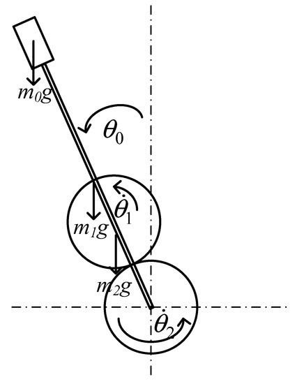
Figure 1.
The structure of a planetary train-type inverted pendulum.
The kinematic relationship between the planetary gears, the sun gear, and the pendulum lies in the mutual movement between the two. First, when the pendulum is stationary (), the ratio between the planetary gear motion and sun gear motion is shown as follows:
where is the sun gear angle, is the planetary gear angle, N1 and N2 present the number of sun gear and planetary gear, respectively, and r1 and r2 are the radii of the sun gear and planetary gear, respectively. Thus, the angular velocity of the planetary gear is derived as follows:
Assume that the center gear is stationary () and the pendulum and planet gear are allowed to rotate. The planetary gear center velocity is derived as follows:
The angular velocity of planetary gear () is as follows:
Equations (3) and (4) are combined and derived as follows:
Lagrangian mechanics were used to obtain relations among input motor torque , center gear , and output of the pendulum . This method can be used to analyze mechanisms in system methods. The potential energy and kinetic of each movable part are derived as follows:
where l is the pendulum length, represent the kinetic energy of the pendulum, planetary gear, and center gear, respectively; P0 and m0 denote the potential energy and the mass of the pendulum, respectively; P1, I1 and m1 and represent the potential energy, the moment of inertia, and the mass of the planetary gear, respectively; and P2 and I2 are the potential energy and the moment of inertia of the center gear, respectively.
From Equation (5), we derive the Lagrangian as follows:
where and are two independent variables, which are generalized coordinates. Moreover, two dynamic equations are derived using the Lagrange equation as follows:
Equation (8) shows that the pendulum is not applied with external torque, therefore zero is assigned to the variable .
3. Structure of a Hierarchical Neural Network
In this section, the structure of a hierarchical neural network is introduced. Figure 2 shows the structure of a multi-level control gene in a layered approach. The value of the first-level control gene controls the activation of the parameter gene. To illustrate the status of the control genes, each open control gene was assigned a value of 1 and each of the closed genes was designated as 0. Although the inactive genes were turned off for a period of time, they still exist in the chromosome. This is called hierarchical chromosome architecture.
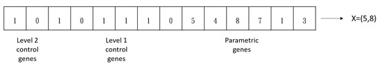
Figure 2.
An example of chromosome representation.
Figure 2 shows that a chromosome comprises six control genes in the form of bits and six parametric genes in the form of integers, where X represents a chromosome with a length of 2 and a solution of 5 and 8. In addition, multi-layered chromosomes are formulated by increasing the level of stratification in the chromosome. Figure 3 illustrates an example of a three-level chromosome.
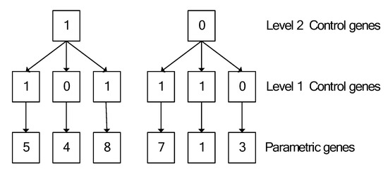
Figure 3.
A three-level chromosome.
A hierarchical chromosome representation is shown in Figure 4. Each chromosome contains a control gene and a connection gene. A control gene in the form of bits activates layers and neurons. A connection gene, which is a real value representation, has connection weights and neuron biases. Figure 5 presents the structure of a hierarchical neural network, where w1, w2, and w3 represent the weights of neural networks.
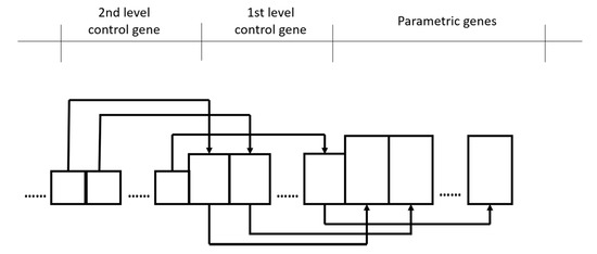
Figure 4.
Hierarchical structure of the chromosome.
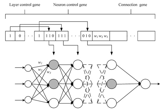
Figure 5.
Structure of a hierarchical neural network.
This particular treatment ensures that the structural chromosome contains both active and inactive genes. Inactive genes remain in the chromosomal structure and can continue to exist in the next generation. In the chromosome, the natural genetic variation avoids falling into local optimization and leads to early convergence. Therefore, it balances the use of its accumulated knowledge with the exploration of new search spaces. In addition, this structure allows for greater genetic variation in the chromosome and allows multiple simultaneous genetic changes to maintain high viability.
4. Proposed Improved Particle Swarm Optimization
This section introduces the review of particle swarm optimization, local search of chaos, and the IPSO algorithm.
4.1. Review of Particle Swarm Optimization (PSO)
In PSO [17,18], the trajectory of each particle is based on its flight experience and search space to update the speed of each particle. The position and speed vector of the ith particle are represented as and , respectively. The optimal position of each particle is defined as , and the optimal position of all particles is defined as . The new speed and position of the particle used for the next evaluation is derived as follows:
where and are acceleration coefficients. Moreover, two separately generated random numbers (i.e., ) are between 0 and 1. The first term in Equation (9) illustrates the speed of the previous generation and provides momentum for the particle search space. The second term in Equation (9) is a cognitive component that facilitates the movement of particles toward their own local optimal positions. The third term in Equation (9) illustrates the social components and synergistic effects of the particle’s global optimal solution.
4.2. Local Search Using Chaotic Method
To improve the searching space and avoid falling into the local minimum, the chaotic method is used in PSO. A logistic equation in [19] was used for developing hybrid PSO and is defined as follows:
where is a control parameter. Although Equation (11) is deterministic, it exhibits chaotic dynamics for and . This equation shows that the initial conditions are very important dependencies on the sensitivity of the chaotic sequence. Subtle differences in the initial values of chaotic variables can cause significant differences in their long-term trajectories. In the search space, the trajectory of chaotic variables can be ergodically traversed. The chaotic local search (CLS) process is defined as follows:
In Equation (12), is kth iteration and is the ith chaotic variable. is set to between 0 and 1 for and .
The CLS process is as follows:
Step 1: Decision variables are located in the interval . The value of is set between 0 and 1 and is shown as follows:
Step 2: Using Equation (12), determine the chaotic variable in the next iteration.
Step 3: The conversion of the chaotic variable turns into the decision variables
Step 4: The evaluation of the new solution is found by using decision variable . If the new solution is superior to the previous solution, then the previous solution is updated as follows:
Step 5: Go to i + 1.
4.3. Proposed Improved Particle Swarm Optimization
Figure 6 shows the parameter adjustment of the chromosome. The control genes are adjusted using a GA [20,21], whereas the parameter genes are tuned using PSO. The GA is a stochastic search procedure based on natural selection with the use of reproduce, crossover, and mutation operations.
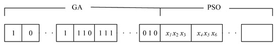
Figure 6.
The adjustable parameters of the chromosome.
The reproduction operation is used to copy individual strings based on the evaluated fitness values. Each individual is assigned a fitness value using a fitness assignment method where a large value indicates satisfactory fitness. In this study, a roulette-wheel selection method [22] was used. The individuals with the optimal performance in the first half of the population [23] are directly reproduced in the next generation. By performing crossover operations for individuals in the first half of the parent generation, the other half of the next generation is generated. For each generation, the reproduction operation keeps the same chromosomes in the first half of the population.
Figure 7 shows the two-point crossover operation. The figure shows the generation of new individuals by exchanging site values between sites selected by parents. Figure 7 shows the two-point crossover operation. The figure shows the generation of new individuals by exchanging site values between the selected sites from parents. When the crossover operation is performed, the unsatisfactory individuals are replaced by the newly generated offspring.
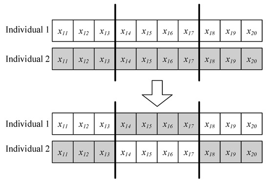
Figure 7.
Two-point crossover operation.
During mutation, the allele of a gene is randomly altered. Figure 8 shows the mutation of an individual. In contrast to conventional symbiotic evolution [22], a mutation value is created using a constant range. In mutation, new genetic materials are used in the population. Because mutation is a random search operation, it must be used sparingly.
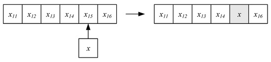
Figure 8.
Mutation operation.
By replicating better control genes in this generation and using them for crossover and mutation operations, the better control genes in the next generation are produced. Therefore, the GA is used to develop a hierarchical neural network. Figure 9 shows the flowchart of the proposed IPSO algorithm. The IPSO algorithm is illustrated as follows:
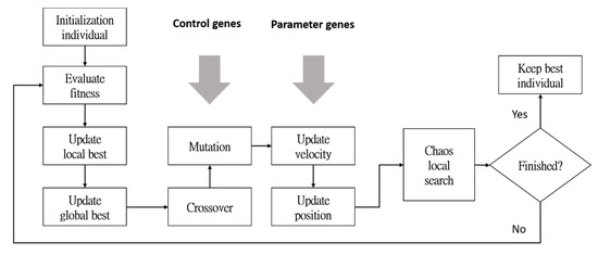
Figure 9.
Flowchart of the proposed improved particle swarm optimization (IPSO) algorithm.
Step 1: Initially, randomly generate P particles forming the swarm.
Step 2: Evaluate the fitness values from each particle.
where RMSE and W_R represents the root mean square error and the weight ratio of connected neurons, respectively; the evaluation ratio and are set as 0.7 and 0.3, respectively.
Step 3: Update the local best particle and the global best particle.
Step 4: Adjust control genes by using reproduce, crossover, and mutation operations.
Step 5: Use Equations (9) and (10) for updating the parameter genes.
Step 6: Use CLS to update the optimal particle.
Step 7: If the learning process has been completed, the best individual is derived. Otherwise, go back to Step 2.
5. Experimental Results
The performance of IPSO-based NNC in practically unstable nonlinear control applications is evaluated using the VisSim environment with a RT-DAC4/PCI motion control card and hardware-in-the-loop. VisSim is a simulation of complex nonlinear dynamic systems in a Windows environment. In this study, based on the VisSim environment, the IPSO-based NNC was implemented in a planetary train inverted pendulum control system.
Figure 10 shows the block diagram of the control system. The encoder was used for sensing the pendulum angle. The angle signal was used as a feedback signal. The motor torque is used to control the swing angle of the pendulum in the equilibrium state to indicate that the control is completed.
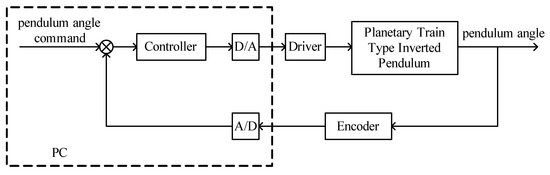
Figure 10.
Block diagram of the control system.
This study compared the proposed IPSO-based NNC with a proportional–integral–derivative (PID) controller, PSO-based NNC, and GA-based NNC. The PID controller is shown in the following:
where u(t) represents the controller’s output and e(t) represents the difference between the controller’s desired and measured values. The control gains obtained through extensive experimental experience are Kp = 830, Ki = 0 and Kd = 0.3284.
5.1. Control of Different Reference Trajectories
To validate the control abilities of the proposed IPSO-based NNC, the set-point and periodic square commands are used as different reference trajectories in this experiment. The initial parameters of the particle swarm optimization are the number of particles, the single inertia weight w, acceleration constants C1 and C2, and number of generations (see Table 1). The different inertia weights will lead to the different performance of the proposed algorithm. Thus, in this study, the inertia weight values were set as 0.3, 0.4, 0.6, 0.8, and 0.9. The performance evaluations of the inertia weight (ω = 0.8) were more efficient than that of the inertia weights (ω = 0.3, 0.4, 0.6 and 0.9). Therefore, the inertia weight (ω = 0.8) was adopted in this study.

Table 1.
Initial parameters of PSO.
Figure 11 presents the real control system of a planetary train inverted pendulum. The performance measurement of the controller comprised set-point regulation and a square command tracking capability. In the set-point command experiment, the proposed method was used to control the inverted pendulum for following the set-point reference. In this study, the set-point reference is equal to zero. Figure 12a–d shows the comparison results of the regulation of IPSO-based NNC, PID controller, PSO-based NNC, and GA-based NNC. In order to validate the performance of set-point regulation, the sum of absolute error (SAE) are defined in the following:
where and represent the actual angle of the pendulum and the referred angle of the pendulum, respectively, and and denote the actual speed of the pendulum and the referred speed of the pendulum, respectively. Table 1 shows the experimental results of the sum of the absolute error for the pendulum angle () and pendulum speed ().
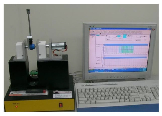
Figure 11.
A real control system of planetary train inverted pendulum.
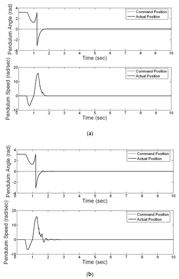
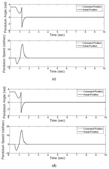
Figure 12.
Regulation comparisons of (a) proposed IPSO-based NNC, (b) PID controller, (c) PSO-based NNC, and (d) GA-based NNC.
In the periodic square wave signal command experiment, we used a square wave with an amplitude of ±0.02 and a frequency of 0.5 Hz to evaluate the tracking ability of the proposed method. Figure 13a–d show the regulation performance of the proposed IPSO-based NNC, PID controller, PSO-based NNC and GA-based NNC, respectively. In this experiment, a sampling rate of 0.1 s is used. Table 2 presents the summary of the experimental results. In this table, the comparison results of various controllers in the set-point and periodic square commands show that the proposed IPSO-based NNC outperforms the other controllers.
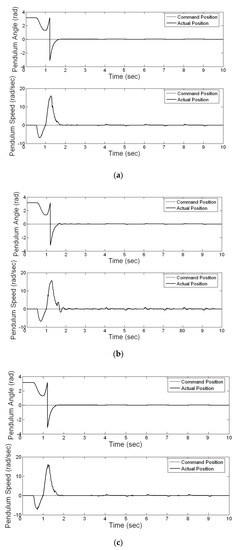
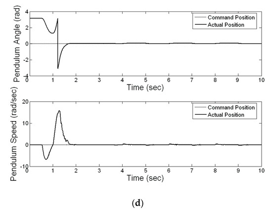
Figure 13.
Tracking comparisons of (a) proposed IPSO-based NNC, (b) PID controller, (c) PSO-based NNC, and (d) GA-based NNC.
Table 2.
Comparison results of various controllers in the set-point and periodic square commands.
5.2. Robustness Test of IPSO-Based NNC
To validate the usefulness of the proposed control system, two different cases, including the influence of impulse noise (i.e., add unknown impulse noise to the plant output) and effect of change in plant dynamics (i.e., add dynamic value to the plant input), are used in this experiment. First, one impulse noise value, 0.1 rad, is added to the plant output at the 10th second when a set-point of 0.04 rad is adopted in this case. Experimental results show that the proposed method recovers quickly when pulse noise occurs, as illustrated in Figure 14a. Second, one general characteristic of many industrial-control processes is that their parameters tend to change in an unpredictable way. In this experiment, 0.5*u (k-0.005) is added to the plant input between the 7th second and the 15th second, in order to test the robustness of the proposed controller. Figure 14b shows the recovering results of the proposed method.
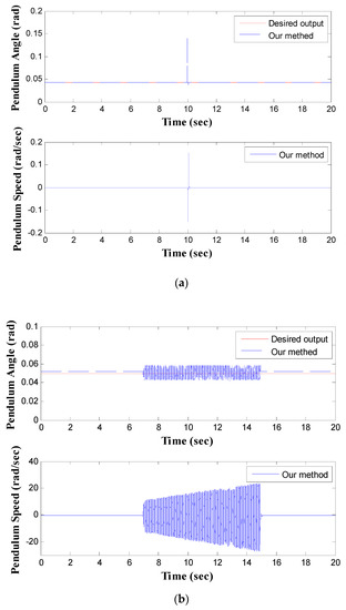
Figure 14.
(a) The effect of one impulse noise, (b) the effect of a change in plant dynamics.
6. Stability Analysis of IPSO-Based NNC
Consider the nth-order nonlinear system (Figure 15) that can be expressed in the canonical form
where f is an unknown continuous function, b is the control gain (For simplicity b = 1 is taken in the subsequent development), and is the input and output of the plant, respectively. We assume that the state vector is available for measurement. The control objective is to force the plant state vector y to follow a specified desired trajectory, yd, under the constraint that all signals involved must be bounded.
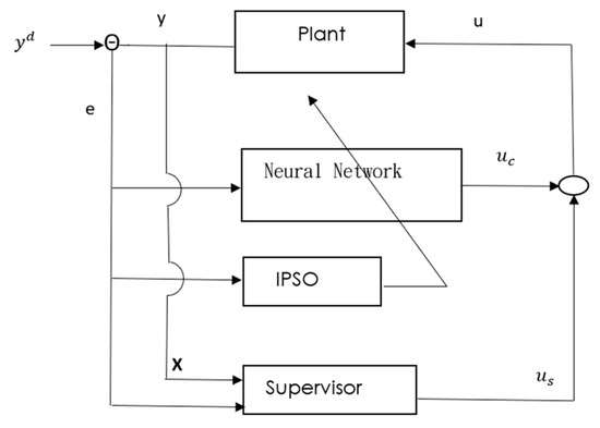
Figure 15.
The overall scheme of stable IPSO-based NNC.
Defining the tracking error vector, the problem is thus to obtain a feedback control law, , where and are control outputs of the NNC controller and the supervisor, respectively.
The global stability of the control system is a basic requirement for solving nonlinear control problems. Because the general evolution algorithm has become characteristic of random search, some search points may cause learning processes to be unstable. In this study, the supervisor is designed (Figure 15) to guarantee global stability of the closed-loop system in the sense that the error state variables must be uniformly bounded, i.e., for all , where D is a design parameter specified by the designer.
Let an error metric be defined , . r(t) = 0 defines a time-varying hyperplane in in which the tracking error vector decays exponentially to zero. The time derivative of the error metric can be expressed as:
where
Considering as the Lyapunov function candidate. According to [24], we can derive the results as follows:
If condition (C > 0 is a constant) is assumed, the supervisory us(t) can be expressed as:
where is a constant; if , and if . Because all terms in Equation (23) can be determined, the supervisory control us(t) can be implemented. Then, substitute Equation (23) into Equation (22) and consider the case, we can derive the results as follows:
Therefore, using the supervisory us(t) in Equation (23), we can derive , i.e., , which in turn implies .
7. Conclusions
This study proposed an IPSO-based NNC for an unstable nonlinear system control. The proposed method can automatically determine the number of hidden levels and neurons and use the chaos method to enhance the ability of PSO to optimize neural network parameters. The proposed IPSO-based NNC was successfully applied to the control system of a planetary train-type inverted pendulum. Experimental results show that the proposed IPSO-based NNC has a smaller SAE than PID controllers, PSO-based NNC, and GA-based NNC. Moreover, the proposed method achieved 3.2% and 2.4% higher performance, respectively, in and than the traditional PSO method.
The trained NNC controller can successfully control an unstable nonlinear system, but the weights of the NNC have no physical meaning. Future works will design a new neural fuzzy network which has learning ability, and its fuzzy rules will have a similar thinking logic to that of humans.
Author Contributions
Revised manuscript, C.-J.L. and X.-Y.L.; conceptualization and methodology, C.-J.L., X.-Y.L. and J.-Y.J.; software, C.-J.L. and X.-Y.L.; writing—original draft preparation, C.-J.L.
Funding
This research was funded by Ministry of Science and Technology of the Republic of China, Taiwan grant number MOST 108-2634-F-005-001.
Conflicts of Interest
The authors declared no potential conflicts of interest with respect to the research, authorship, and/or publication of this article.
References
- Maksimenko, V.A.; Kurkin, S.A.; Pitsik, E.N.; Musatov, V.Y.; Runnova, A.E.; Efremova, T.Y.; Hramov, A.E.; Pisarchik, A.N. Artificial Neural Network Classification of Motor-Related EEG: An Increase in Classification Accuracy by Reducing Signal Complexity. Complexity 2018, 2018. [Google Scholar] [CrossRef]
- Yang, X.C.; Yung, M.H.; Wang, X. Neural-network-designed pulse sequences for robust control of singlet-triplet qubits. Phys. Rev. A 2018, 97, 042324. [Google Scholar] [CrossRef]
- Eggensperger, K.; Lindauer, M.; Hutter, F. Neural Networks for Predicting Algorithm Runtime Distributions. Int. Jt. Conf. Artif. Intell. 2018, 1442–1448. [Google Scholar] [CrossRef]
- Waghulde, N.P.; Patil, N.P. Genetic Neural Approach for Heart Disease Prediction. Int. J. Adv. Comput. Res. 2014, 4, 778–784. [Google Scholar]
- Zhining, Y.; Yunming, P. The Genetic Convolutional Neural Network Model Based on Random Sample. Int. J. U E Serv. Sci. Technol. 2015, 8, 317–326. [Google Scholar]
- Li, L.; Lin, C.J.; Huang, M.L.; Kuo, S.C.; Chen, Y.-R. Mobile Robot Navigation Control Using Recurrent Fuzzy CMAC Based on Improved Dynamic Artificial Bee Colony. Adv. Mech. Eng. 2016, 8, 1–10. [Google Scholar] [CrossRef]
- Turabieh, H. A Hybrid ANN-GWO Algorithm for Prediction of Heart Disease. Am. J. Oper. Res. 2016, 6, 136–146. [Google Scholar] [CrossRef]
- Chen, J.F.; Do, Q.H.; Hsieh, H.N. Training Artificial Neural Networks by a Hybrid PSO-CS Algorithm. Algorithms 2015, 8, 292–308. [Google Scholar] [CrossRef]
- Jhang, J.Y.; Lin, C.J.; Lin, C.T.; Young, K.Y. Navigation Control of Mobile Robots through an Interval Type-2 Fuzzy Controller Based on Dynamic-Group Particle Swarm Optimization. Int. J. Control Autom. Syst. 2018, 16, 2446–2457. [Google Scholar] [CrossRef]
- Liu, B.; Wang, L.; Jin, Y.H.; Tang, F.; Huang, D.X. Improved Particle Swarm Optimization Combined with Chaos. Chaos Solitons Fractals 2005, 25, 1261–1271. [Google Scholar] [CrossRef]
- Tang, K.S.; Man, K.F.; Liu, Z.F.; Kwong, S. Minimal Fuzzy Memberships and Rules Using Hierarchical Genetic Algorithms. IEEE Trans. Ind. Electron. 1998, 45, 162–169. [Google Scholar] [CrossRef]
- Ping, Z. Tracking problems of a spherical inverted pendulum via neural network enhanced design. Neurocomputing 2013, 106, 137–147. [Google Scholar] [CrossRef]
- Al-Araji, A.S. An Adaptive Swing-up Sliding Mode Controller Design for a Real Inverted Pendulum System Based on Culture-Bees Algorithm. Eur. J. Control 2019, 45, 45–56. [Google Scholar] [CrossRef]
- Magdy, M.; Marhomy, A.E.; Attia, M.A. Modeling of inverted pendulum system with gravitational searchalgorithm optimized controller. Ain Shams Eng. J. 2019, 10, 129–149. [Google Scholar] [CrossRef]
- Su, X.; Xia, F.; Liu, J.; Wu, L. Event-triggered fuzzy control of nonlinear systems with its application to inverted pendulum systems. Automatica 2018, 94, 236–248. [Google Scholar] [CrossRef]
- Cho Chieh Tech. Enterprise Ltd. 2015. Available online: http://www.chochieh.com.tw (accessed on 8 October 2018).
- Chiou, J.S.; Tran, H.K.; Shieh, M.Y.; Nguyen, T.N. Particle Swarm Optimization Algorithm Reinforced Fuzzy Proportional-integral-derivative for a Quadrotor Attitude Control. Adv. Mech. Eng. 2016, 8, 1–7. [Google Scholar] [CrossRef]
- Lee, H.; Kim, K.; Kwon, Y.; Hong, E. Real-Time Particle Swarm Optimization on FPGA for the Optimal Message-Chain Structure. Electronics 2018, 7, 274. [Google Scholar] [CrossRef]
- Tsai, J.T.; Liu, T.K.; Chou, J.H. Hybrid Taguchi-Genetic Algorithm for Global Numerical Optimization. IEEE Trans. Evolut. Comput. 2004, 8, 365–377. [Google Scholar] [CrossRef]
- Idrissi, J.; Hassan, R.; Youssef, G.; Mohamed, E. Genetic Algorithm for Neural Network Architecture Optimization. In Proceedings of the 2016 3rd International Conference on Logistics Operations Management (GOL), Fez, Morocco, 23–25 May 2016. [Google Scholar] [CrossRef]
- Islam, B.; Baharudin, Z.; Raza, M.Q.; Nallagownden, P. Optimization of Neural Network Architecture Using Genetic Algorithm for Load Forecasting. In Proceedings of the 2014 5th International Conference on Intelligent and Advanced Systems (ICIAS), Kuala Lumpur, Malaysia, 3–5 June 2014. [Google Scholar] [CrossRef]
- Kumar, R.; Jyotishree. Blending Roulette Wheel Selection & Rank Selection in Genetic Algorithms. Int. J. Mach. Learn. Comput. 2012, 2, 365–370. [Google Scholar]
- Lin, H.Y.; Lin, C.J.; Huang, M.L. Optimization of Printed Circuit Board Component Placement Using an Efficient Hybrid Genetic Algorithm. Appl. Intell. 2016, 45, 622–637. [Google Scholar] [CrossRef]
- Wang, L.X. Stable adaptive fuzzy control of nonlinear systems. IEEE Trans. Fuzzy Syst. 1993, 1, 146–155. [Google Scholar] [CrossRef]


© 2019 by the authors. Licensee MDPI, Basel, Switzerland. This article is an open access article distributed under the terms and conditions of the Creative Commons Attribution (CC BY) license (http://creativecommons.org/licenses/by/4.0/).